Article

Transverse Electric Guided Wave Propagation in a Plane Waveguide with Kerr Nonlinearity and Perturbed Inhomogeneity in the Permittivity Function

Department of Mathematics and Supercomputing, Penza State University, 440026 Penza, Russia
*
Author to whom correspondence should be addressed.
Photonics 2023, 10(4), 371; https://doi.org/10.3390/photonics10040371
Submission received: 5 March 2023 / Revised: 21 March 2023 / Accepted: 24 March 2023 / Published: 27 March 2023

Abstract

:
The paper focuses on the problem of transverse electric wave propagation in a plane-shielded waveguide filled with a nonhomogeneous and nonlinear (Kerr) medium. The nonlinear part of the permittivity is characterized by the Kerr law in the focusing regime, while its linear part is a constant that is perturbed by a small continuous function. Such perturbation can be considered to be an attempt to take into account the inevitable presence of impurities in the medium, causing slight deviations in the dielectric permittivity. In the paper, the existence of solutions to the considered problem is proved, including solutions with and without linear counterparts. Some numerical results are presented as well.

1. Introduction

The theory of guided waves, including electromagnetic cases, is one of the fruitful sources of novel mathematical problems. The classical theory of guided electromagnetic waves in plane dielectric waveguides and films with linear homogeneous and nonhomogeneous fillings was well developed many years ago [1,2,3].
Sufficiently high-power optical processes are often nonlinear, and this nonlinearity cannot be ignored [4,5,6,7,8]. This fact results in the wide and deep study of nonlinear optical processes and, in particular, the vast development of nonlinear guided wave optics [6,7,9,10,11,12]. The simplest nontrivial problems, in this case, are problems of propagation of a monochromatic transverse electric (TE) electromagnetic wave in a plane waveguide filled with a homogeneous nonlinear medium [6,13,14,15]. The best known (and in some senses the most studied) is the so-called Kerr medium, i.e., the medium with dielectric permittivity of the form
ε = ε 1 + α | E | 2 ,
where ε 1 and α are real constants, and E is the electric field [4,6,13,14,15,16,17]. Usually, it is assumed that ε 1 > 0 , negative α corresponds to the defocusing Kerr effect, and positive α corresponds to the focusing Kerr effect.
However, real waveguides are never filled with an absolutely homogeneous medium; in any medium, there is always some concentration of impurities that causes slight deviations in the dielectric permittivity. To take into account the discussed effect, one can modify Formula (1) in the following way
ε = ε 1 + β ε 2 + α | E | 2 ,
where β is a real constant that is supposed to be small, and ε 2 is a continuous function with respect to spatial variables. The term β ε 2 in (2) simulates slight deviations in the dielectric permittivity of the medium.
The governing equations for TE waves and the Kerr medium can be solved exactly using elliptic functions [6,13] if β = 0 . The case when the permittivity depends on the field as well as on coordinates is much more complicated. In particular, for TE waves and nonlinearity (2), exact solutions to the governing equations of the problem cannot be found.
In many cases, for nonlinear processes, perturbation approaches can effectively be applied, i.e., in fact, instead of finding solutions to a nonlinear problem, one uses solutions to a linear problem taking into account some corrections [18,19,20]. Such approaches work well if only small corrections are needed. However, corrections can be greater than what is allowed using a perturbation approach, and therefore such an approach cannot be applied. In addition, if a perturbation approach is based on a linear problem, then one can only find solutions to a nonlinear problem that have linear counterparts. This means that if the nonlinear problem has so-called nonperturbative solutions, then one is forced to use other approaches.
This paper focuses on the problem of the propagation of monochromatic TE waves in a plane-shielded waveguide filled with a nonlinear nonhomogeneous medium with permittivity (2), where ε 1 , α are positive constants, β is a real constant and | β | is assumed to be sufficiently small and ε 2 ε 2 ( x ) is a continuous function, where x is the transversal direction of the waveguide. This problem has solutions with as well as without linear counterparts. In this paper, we suggest some modification of a perturbation method based on the usage of solutions to a simpler nonlinear problem (with β = 0 ) in order to find solutions to the original one. Such an approach allows one to prove the existence of eigenvalues (propagation constants) of the waveguiding problem including the ones that do not have linear counterparts.
For waveguiding problems, the main question is to prove the existence of so-called propagation constants (PCs), i.e., the full set of the guided waves that the waveguide supports. From a mathematical standpoint, one needs to solve a boundary eigenvalue problem for the governing equations with appropriate boundary conditions. In this paper, we prove the existence of the PCs (or eigenvalues) and carry out a few numerical experiments.

2. Materials and Methods

Although the paper focuses on the analytical study of the problem, some numerical results are presented as well; see Section 3.4. The description of numerical methods used in this study is given in Section 3.4. All numerical methods are implemented with the package Maple.

3. Results

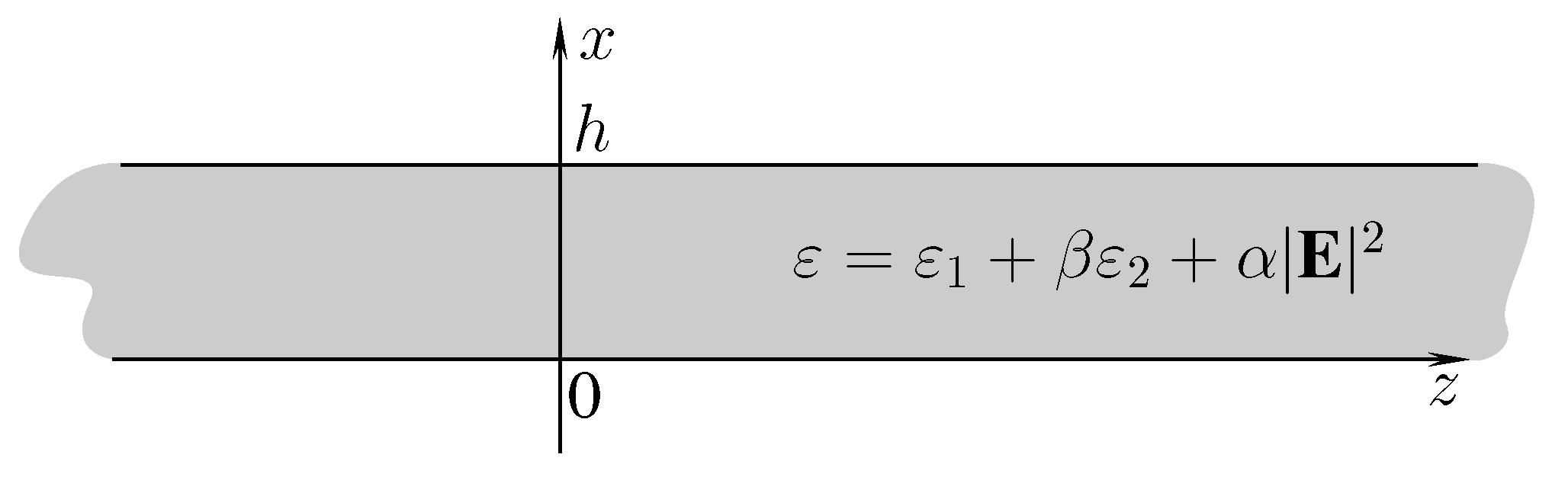
3.1. Statement of the Problem

We consider a monochromatic electromagnetic TE wave ( E , H ) e i ω t , where
E = 0 , E y ( x ) , 0 e i γ z , H = H x ( x ) , 0 , H z ( x ) e i γ z
are electric and magnetic fields, ω is circular frequency, and γ is an unknown real parameter that propagates in the plane waveguide Σ : = { ( x , y , z ) R 3 : 0 x h , ( y , z ) R 2 } which has absolutely conducted walls at both boundaries.
The permittivity ε in layer Σ has the form ε = ε 1 + β ε 2 + α | E | 2 , where ε 1 , α are positive constants, β is a real constant, and | β | is assumed to be sufficiently small, and ε 2 ε 2 ( x ) is a continuous function for x [ 0 , h ] . The permeability is μ = μ 0 , where μ 0 is the permeability of free space. The geometry of the problem is shown in Figure 1.
Fields (3) satisfy Maxwell’s equations
r o t H = i ω ε 0 ε E , r o t E = i ω μ H ,
where ε 0 is a constant (permittivity of free space). The tangential component E y of the electric field vanishes at the absolutely conducted walls. Besides this, we assume that the tangential component H z of the magnetic field is fixed at the boundary x = 0 .
Problem P is to find γ such that there exist fields (3) satisfying Maxwell’s Equation (4) and the above-listed conditions; such values γ are called propagation constants of the waveguide (or eigenvalues of problem P ).
Substituting fields (3) into Equation (4), one obtains
i γ H x H z = i ω ε ε 0 E y , γ E y = ω μ H x , E y = i ω μ H z .
Expressing H x and H z from the second and third equations, respectively, and substituting them into the first equation, one arrives at the following equation
E y ( x ) = γ 2 E y ( x ) ω 2 ε 0 μ 0 ε 1 + β ε 2 ( x ) + α E y 2 ( x ) E y ( x ) .
Let us introduce the notation
k 0 2 = ω 2 ε 0 μ 0
and perform the normalization in accordance with the formulas x ˜ = k 0 x , γ ˜ = k 0 1 γ , h ˜ = k 0 h . Using the notation E y : = u and omitting the tilde symbol, one can rewrite (6) in the form
u ( x ) = ( ε 1 + β ε 2 ( x ) γ 2 ) u ( x ) α u ( x ) 3 .
The third equation of system (5) expresses the link between the tangential component H z of the magnetic field and the first derivative E y of the tangential component E y of the electric field. Taking into account the performed normalization by k 0 , one obtains
u ( x ) = μ 0 ϵ 0 i H z ( x ) = 120 π i H z ( x ) .
From the conditions imposed on fields (3) and the above link between u and component H z , one obtains the following boundary conditions
u ( 0 ) = 0 , u ( 0 ) = A ,
u ( h ) = 0 ,
where A 0 is a real constant connected with the value of component H z at the boundary x = 0 by the relation A = 120 π i H z ( 0 ) .
Please note that u ( x ) satisfies Equation (8) and u ( 0 ) = A , then u ( x ) with u ( 0 ) = A also satisfies Equation (8); for this reason, it is enough to consider only the case where A > 0 in (9). Besides this, if a couple ( γ , u ) satisfies Equation (8) and conditions (9), (10), then the couple ( γ , u ) also satisfies Equation (8) and conditions (9), (10); for this reason, it is enough to consider only the case γ > 0 .
From a mathematical point of view, physical problem P = P α β of wave propagation is equivalent to the problem of finding γ = γ ^ > 0 such that there exists twice the continuous differentiable on [ 0 , h ] function u ( x ) satisfying Equation (8) and conditions (9), (10). We call the looked-for values γ = γ ^ propagation constants (or eigenvalues) and we call the corresponding functions u ( x ; γ ^ ) eigenmodes (or eigenfunctions) of problem P . We often omit the dependence of function u on α , β , γ if it does not lead to misunderstanding.
If β = 0 , one obtains problem P α , which is a special case of problem P . Problem P α is to find γ = γ ¯ > 0 such that there exists function v v ( x ; γ ¯ , α ) satisfying equation
v ( x ) = ( ε 1 γ 2 ) v ( x ) α v 3 ( x ) ,
and boundary conditions
v ( 0 ; γ , α ) = 0 , v ( 0 ; γ , α ) = A ,
v ( h ; γ , α ) = 0 ,
where A is the same as in condition (9). The value γ ¯ is called a propagation constant and function u is called an eigenmode of problem P α .
Problem P α is quite well studied [21,22,23] and we use the main properties of its solutions to solve problem P . To be more precise, we prove that if γ = γ ¯ is a solution to problem P α , then there exists a constant β 0 > 0 such that for any β , where | β | < β 0 , problem P has at least one solution γ = γ ^ in the vicinity of γ ¯ and lim β 0 γ ^ = γ ¯ .
If α = 0 then problem P degenerates into the linear problem P 0 , where β is not necessarily equal to zero, which is to find γ = γ ˜ such that there exists a nontrivial solution w w ( x ; γ ˜ , β ) to equation
w ( x ) = ( ε 1 + β ε 2 ( x ) γ 2 ) w ( x ) ,
satisfying boundary conditions
w ( 0 ; γ , β ) = 0 ,
w ( h ; γ , β ) = 0 .
The value γ ˜ is called a propagation constant and the corresponding function v is called an eigenmode of problem P 0 .
Please note that the second condition in (9), which is necessary to determine discrete propagation constants in (nonlinear) problem P as well as in (nonlinear) problem P α , is unnecessary in the linear problem, and, for this reason, it is omitted.
Problem P 0 is classical in the linear waveguide theory [1,24,25]. The following result takes place.
Statement 1.
Problem P 0 has a finite number of propagation constants γ ˜ . Moreover, if β = 0 , then all positive propagation constants γ ˜ belong to the interval ( 0 , ε 1 ) .
We omit the proof as this result is a part of classical Sturm–Liouville theory [26].
Problem P 0 can be used to develop a standard perturbation approach to find solutions to problem P . Indeed, let γ ˜ be a propagation constant of problem P 0 . It can be shown that for sufficiently small α in some vicinity of γ ˜ there is at least one propagation constant γ ^ of problem P and lim α + 0 γ ^ = γ ˜ .
Obviously, this approach allows one to only find propagation constants of problem P , which have linear counterparts (in other words, those which can be linearized). However, problem P can have solutions without linear counterparts (so-called nonperturbative nonlinear solutions). Such solutions cannot be found using the discussed approach. Indeed, since problem P α has infinitely many nonperturbative solutions [21,22,23], then it is natural to expect the existence of nonperturbative solutions to problem P at least for small (positive) α .

3.2. Problem P α

To develop our approach, we need to present some known results on problem P α . This problem is very deeply studied in [21,22,23]; using the results presented in the cited papers, we easily obtain the following facts.
Statement 2.
The Cauchy problem for Equation (11) with conditions (12) is globally uniquely solvable, and its solution v v ( x ; γ , α ) depends continuously on x , γ , α , where x [ 0 , h ] and α , γ > 0 .
It is clear that solution v ( x ; γ , α ) to the Cauchy problem (11), (12) is an eigenmode of problem P α if it satisfies condition (13). Therefore, one obtains the following quite obvious result.
Statement 3.
Value γ = γ ¯ is a propagation constant of problem P α if and only if it satisfies the characteristic equation
v ( h ; γ , α ) = 0 ,
where v ( x ; γ , α ) is the above-mentioned solution to the Cauchy problem (11), (12).
We call function v ( h ; γ , α ) the characteristic function of problem P α .
Theorem 1.
Problem P α has infinitely many positive propagation constants γ = γ ¯ with the accumulation point at infinity. In addition, among all propagation constants of the problem, there is an infinite number of propagation constants γ ¯ k , where k = 1 , 2 , , such that for any of them there exists a vicinity Γ k = ( γ ¯ k δ k , γ ¯ k + δ k ) , where δ k > 0 is a constant, and on the opposite ends of Γ k there is the inequality
v ( h ; γ ¯ k δ k , α ) · v ( h ; γ ¯ k + δ k , α ) < 0
holds, where v is defined in (17) and Γ k does not contain other propagation constants except γ ¯ k .
We stress that problem P α has infinitely many propagation constants without linear counterparts. Such propagation constants correspond to a novel guided regime arising due to the Kerr effect.

3.3. Problem P

In the beginning, we prove the global unique solvability of the Cauchy problem for Equation (8) with initial conditions (9).
Statement 4.
For γ [ 0 , γ 0 ] and α ( 0 , α 0 ) , where γ 0 , α 0 > 0 are constants, there exists β 0 > 0 such that the Cauchy problem for Equation (8) with conditions (9) is globally uniquely solvable and its solution u u ( x ; γ , α , β ) depends continuously on x , γ , α , β for x [ 0 , h ] and γ [ 0 , γ 0 ] , α ( 0 , α 0 ) , | β | < β 0 .
It is clear that the above-mentioned solution u ( x ; γ , α , β ) to the Cauchy problem (8), (9) is an eigenmode of problem P if it satisfies the condition (10). Therefore, one obtains the following result.
Statement 5.
Value γ = γ ^ is a propagation constant of problem P if and only if it satisfies to the characteristic equation
u ( h ; γ , α , β ) = 0 ,
where u ( x ; γ , α , β ) is the above-mentioned solution to the Cauchy problem (8), (9).
We call function u ( h ; γ , α , β ) the characteristic function of problem P .
Now, we need one more result for the solution u ( x ; γ , α , β ) to the Cauchy problem (8), (9) and solution v ( x ; γ , α ) to the Cauchy problem (11), (12). The following result takes place:
Statement 6.
Let u ( x ; γ , α , β ) be a solution to the Cauchy problem (8), (9), and v ( x ; γ , α ) be a solution to the Cauchy problem (11), (12). Then, for β 0 , it is true that
u ( x ; γ , α , β ) v ( x ; γ , α ) ,
uniformly on x [ 0 , h ] and γ [ 0 , γ 0 ] for fixed α ( 0 , α 0 ) .
We note that results presented in Theorems 4 and 6 are based on the classical theorem of the ordinary differential equation theory, which states that if a Cauchy problem has a unique globally defined solution, then another Cauchy problem with the same initial data and regular small perturbation in the equation also has a unique continuous solution defined globally on the same segment [27].
Everywhere below, we assume that γ Γ , where Γ = [ 0 , γ 0 ] and γ 0 > 0 is a sufficiently large constant, i.e., the segment Γ contains at least n propagation constants γ ^ of problem P α satisfying property (18). The existence of such solutions is guaranteed by Theorem 1.
Subtracting the characteristic function v ( h ; γ , α ) of problem P α from the both sides of (19), one obtains
u ( h ; γ , α , β ) v ( h ; γ , α ) = v ( h ; γ , α ) .
Studying Equation (20), one arrives at the main result.
Theorem 2.
Let problem P α have n solutions γ ¯ k Γ , where k = 1 , n ¯ , satisfying property (18). Then, there exists β 0 > 0 such that for any β ( β 0 , β 0 ) problem P has at least one solution γ ^ k in the vicinity of γ ¯ k and lim β 0 γ ^ k = γ ¯ k for each k = 1 , n ¯ .
In view of Theorem 2 we should give the following comments.
Theorem 2 states the existence of n solutions to problem P if problem P α has n solutions in Γ and | β | is sufficiently small. Here, integer n can be as large as needed but it affects the upper bound β 0 of possible values of β ; namely, the larger the n, the smaller the β 0 . Trying to pass to the limit n + , one obtains β 0 0 ; in other words, in this case, problem P degenerates into problem P α .
If γ 0 is sufficiently large, then at least some of the propagation constants γ ¯ k Γ do not have linear counterparts. This means that those propagation constants γ ^ k for which lim β 0 γ ^ k = γ ¯ k , where γ ¯ k Γ is nonlinearizable, are also nonlinearizable.

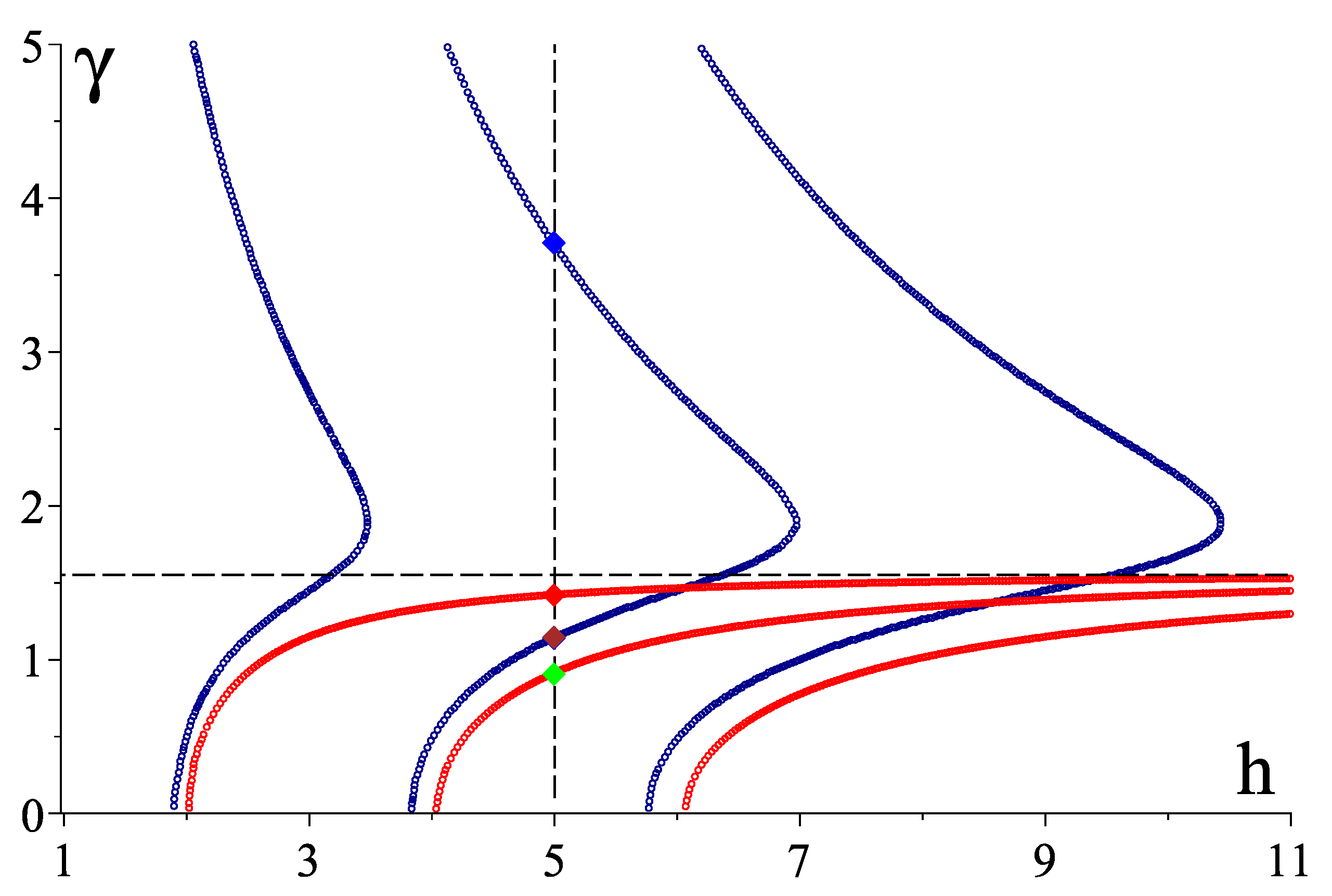
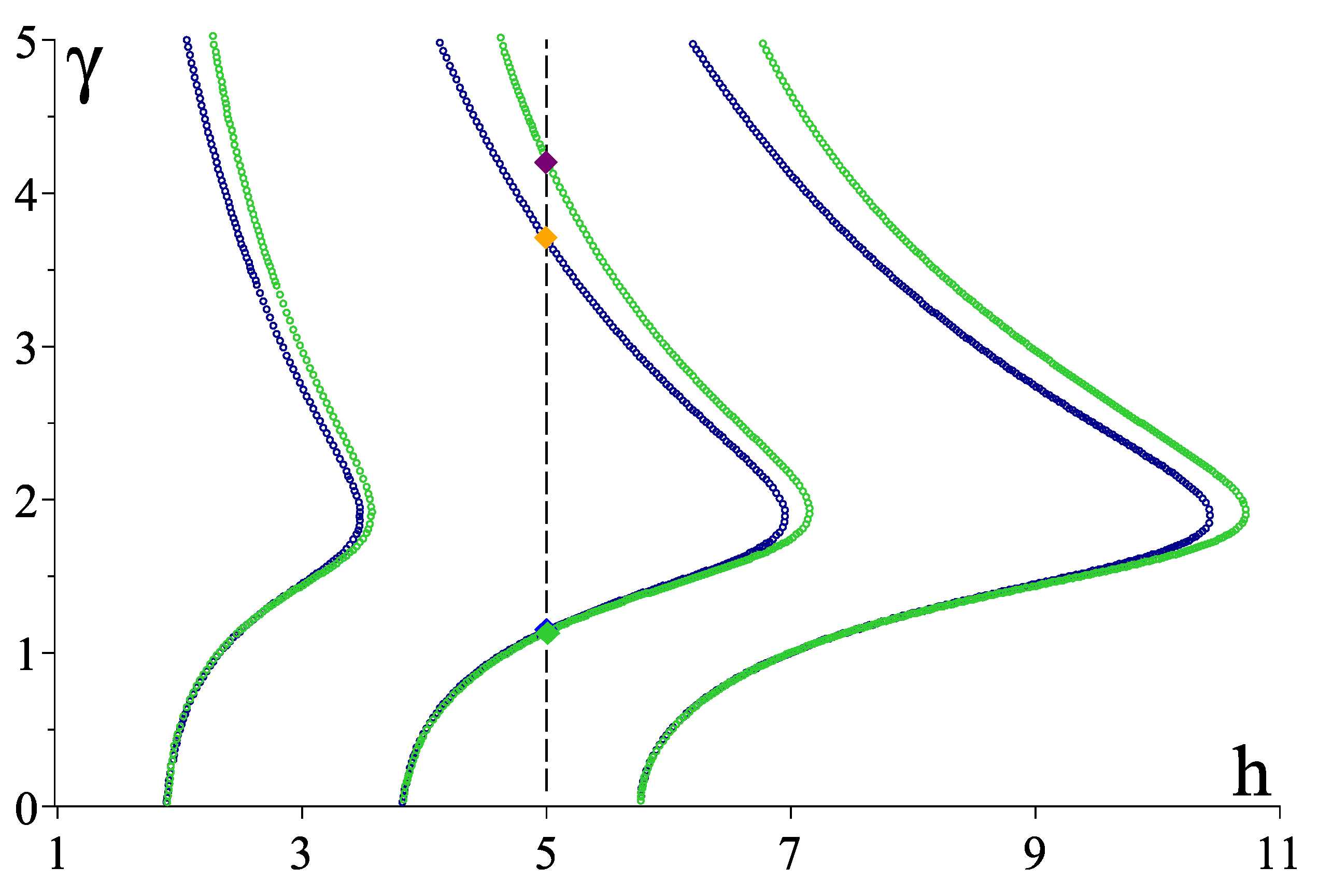
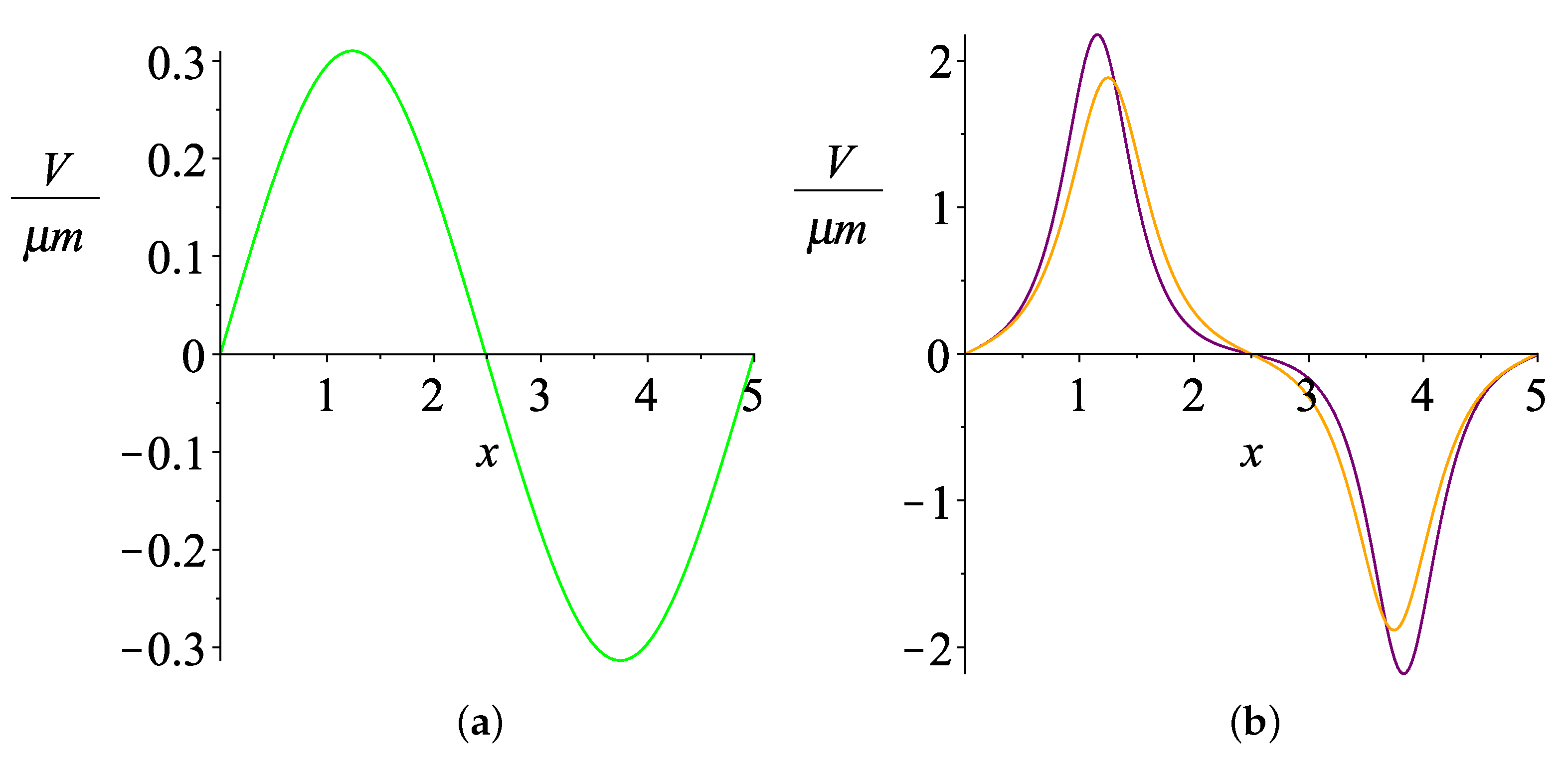
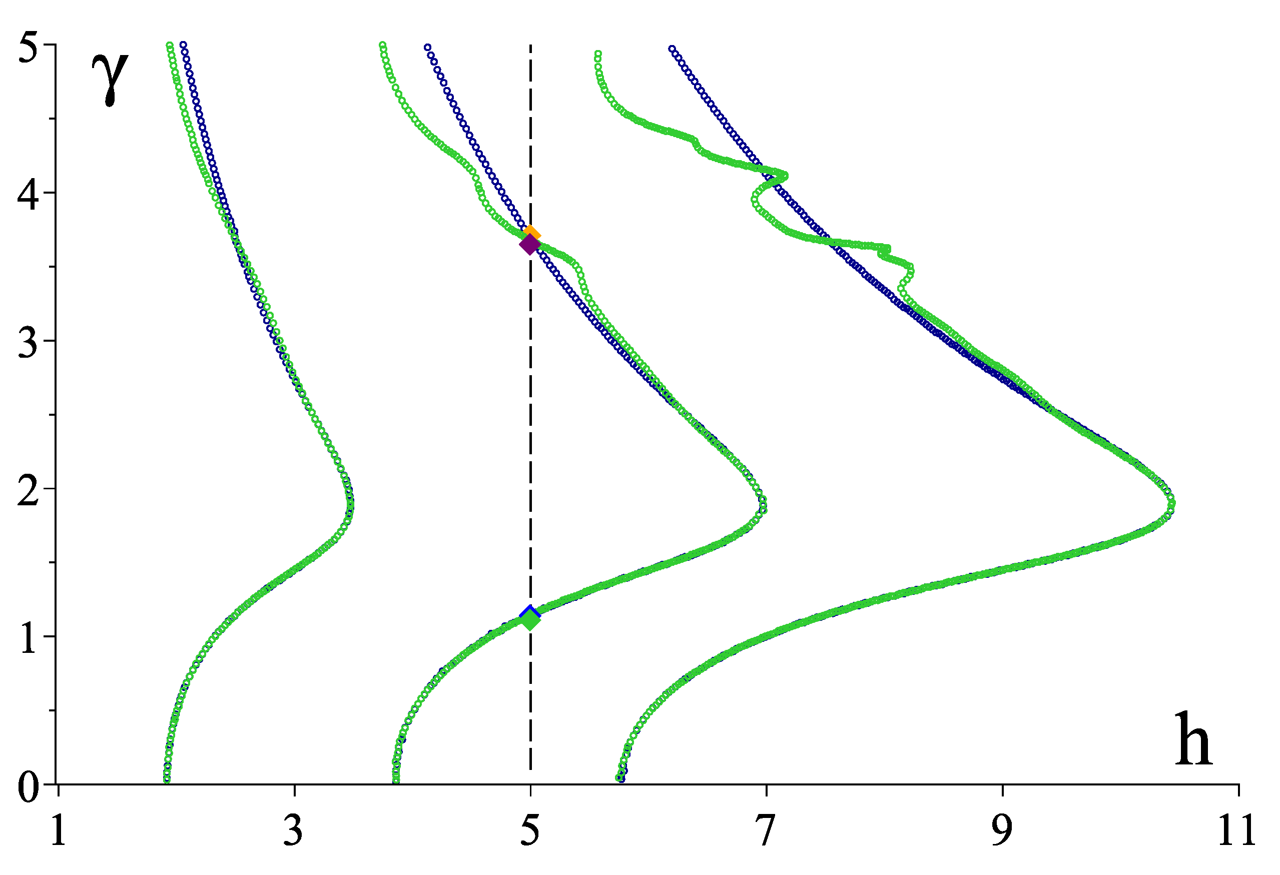
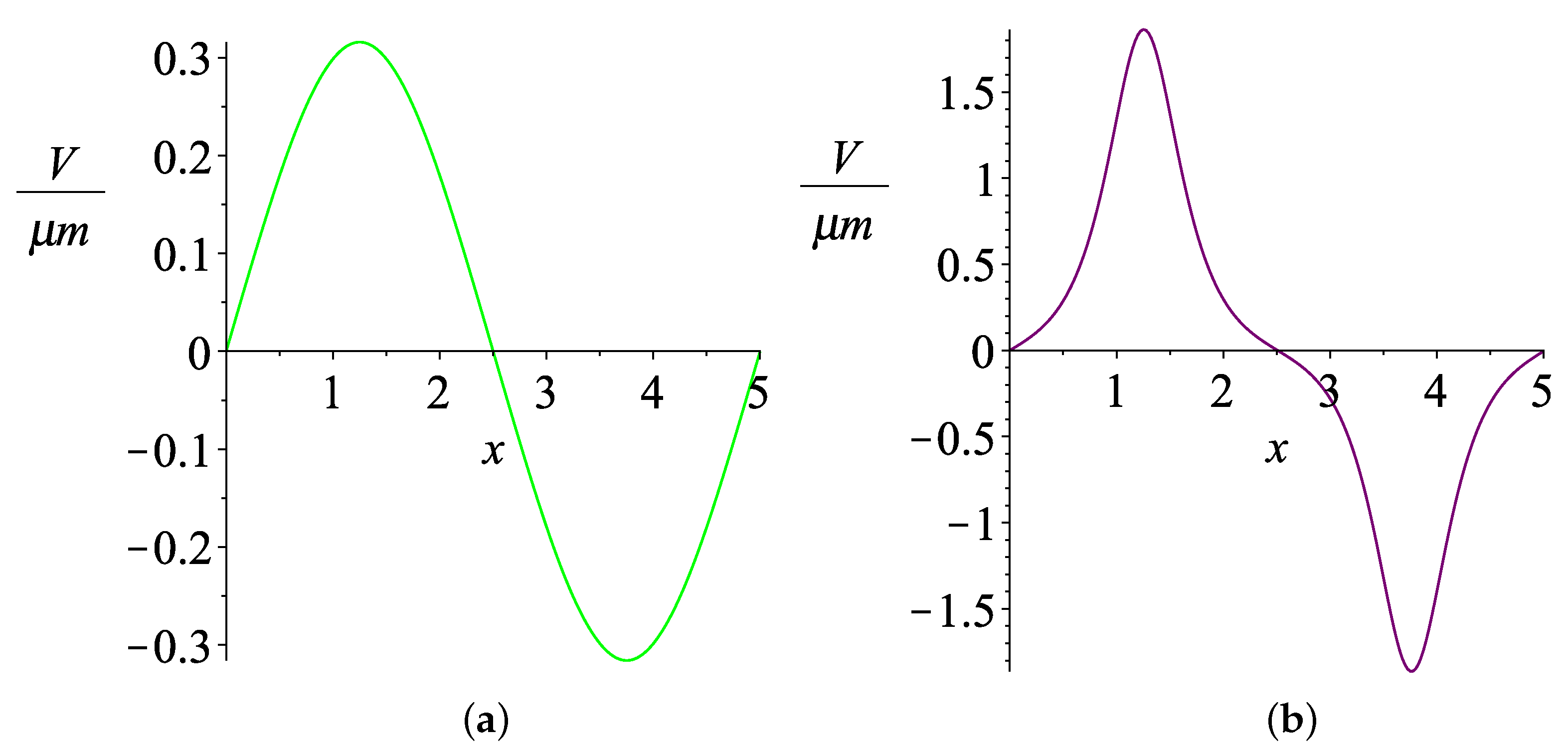
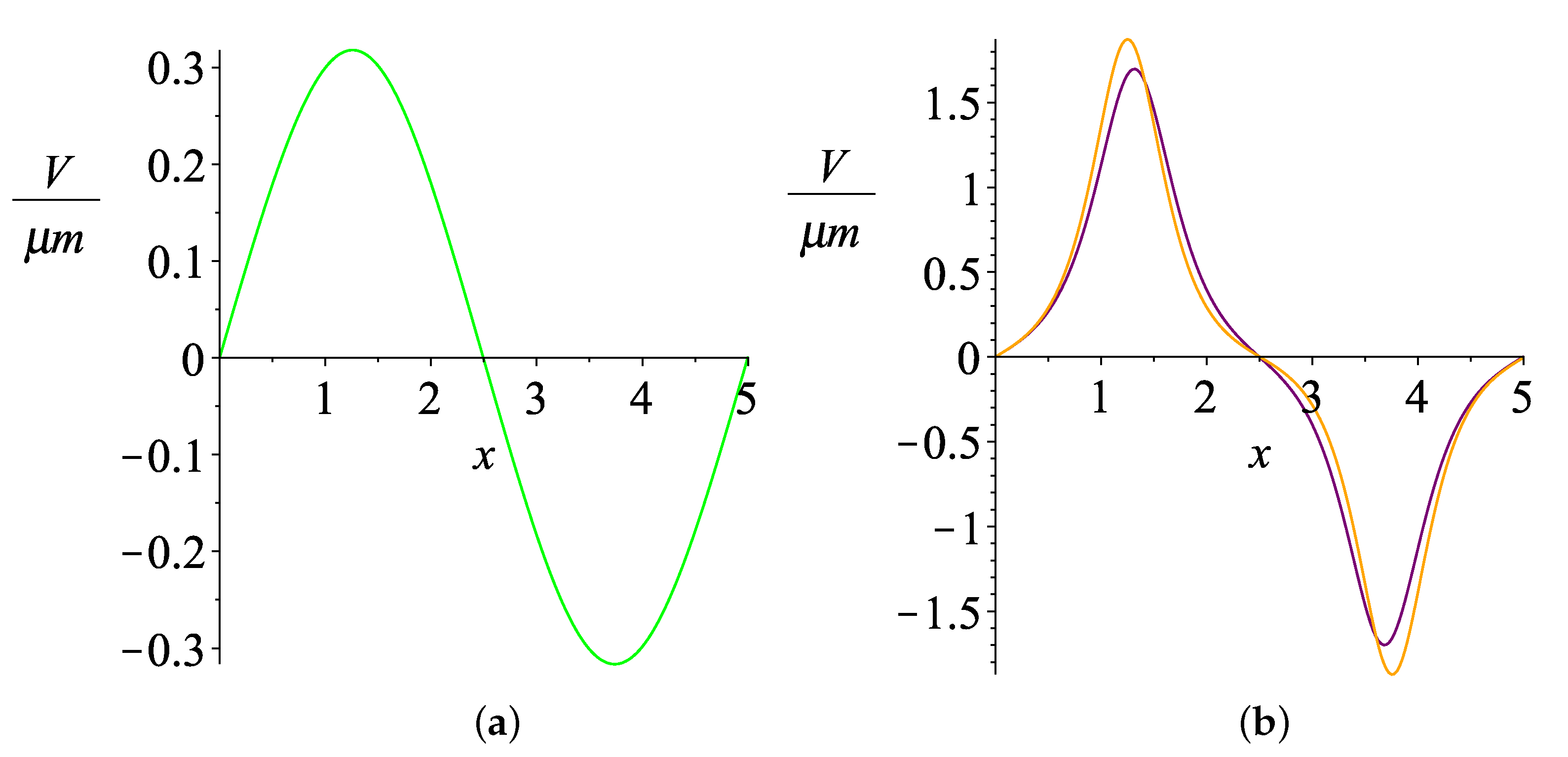
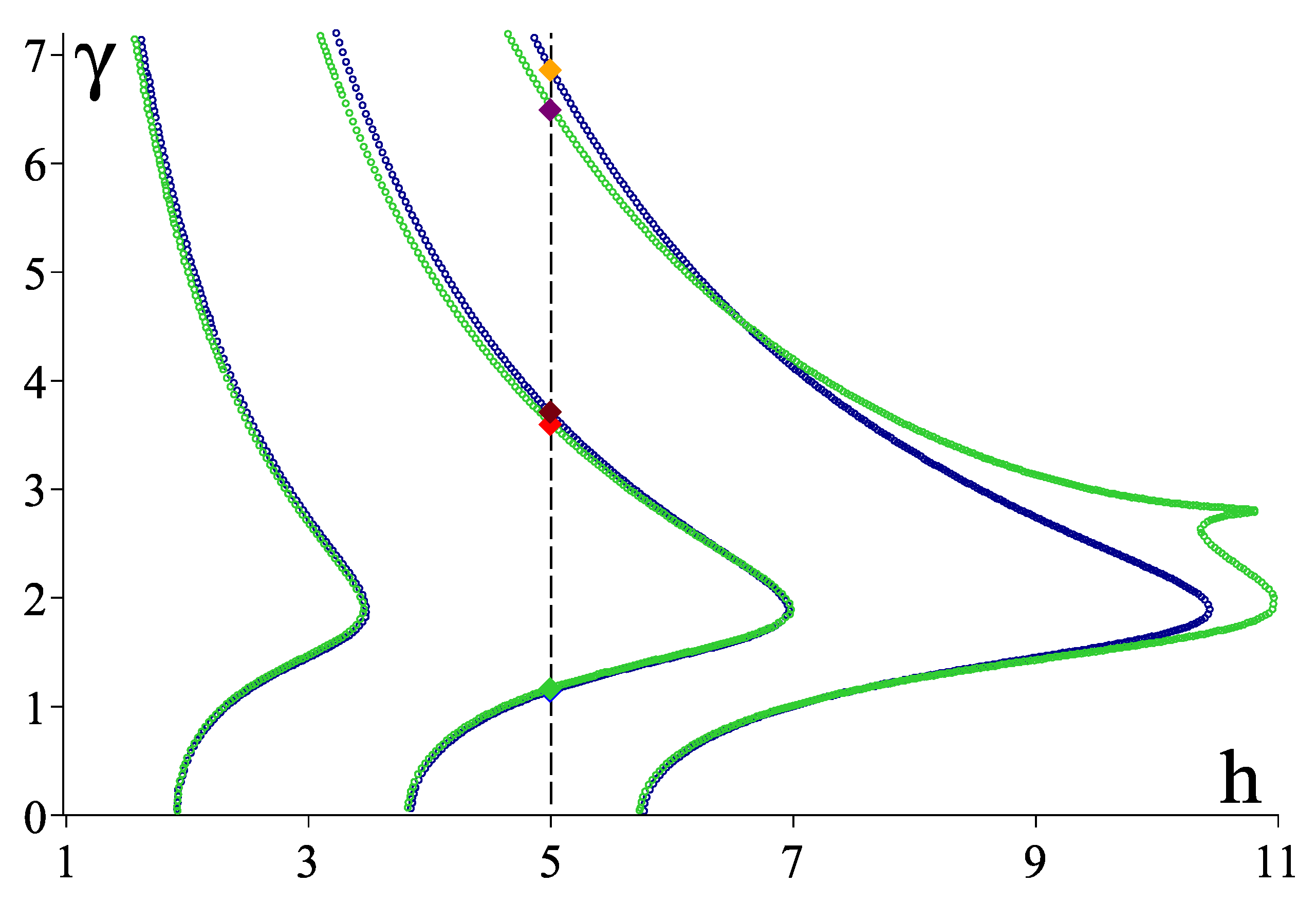
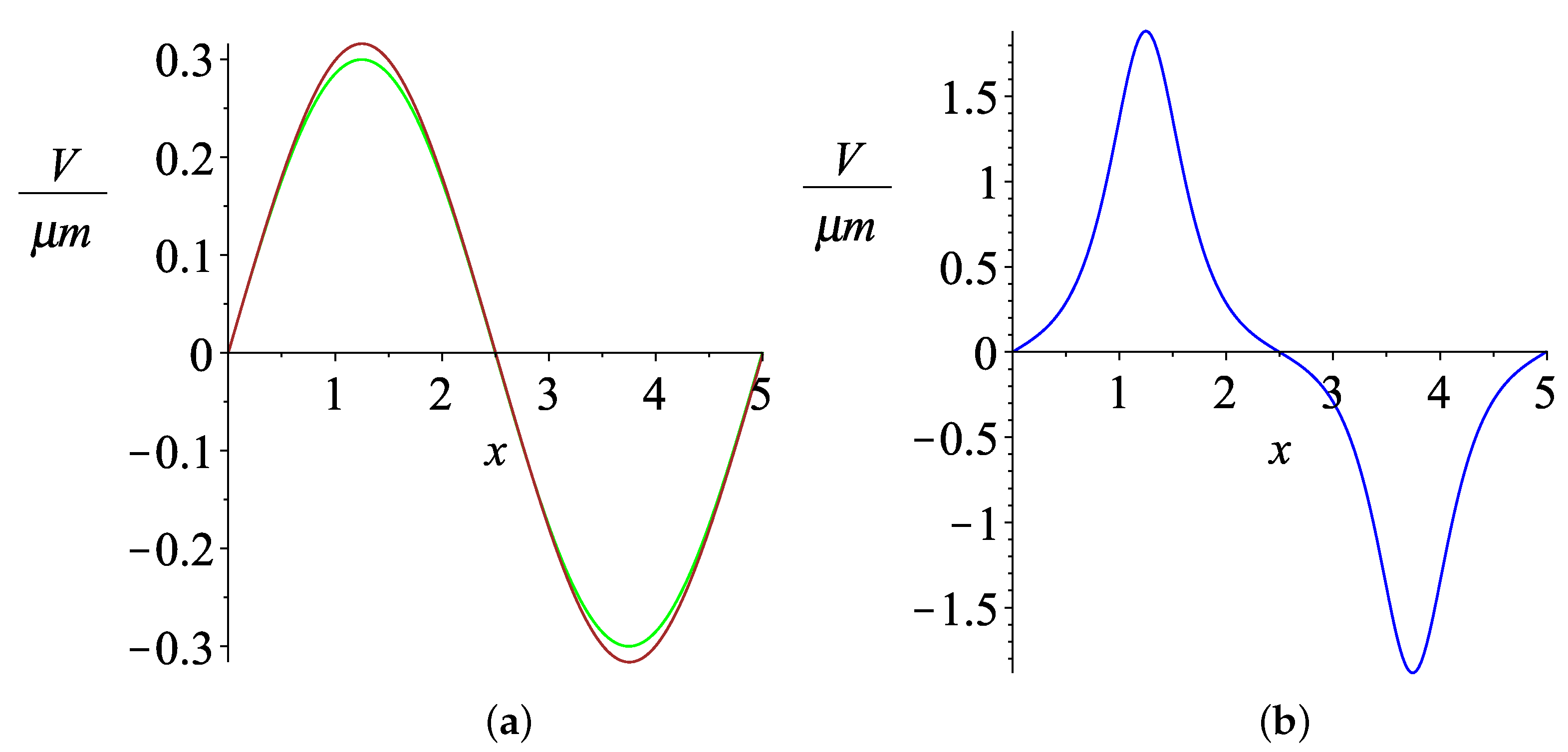
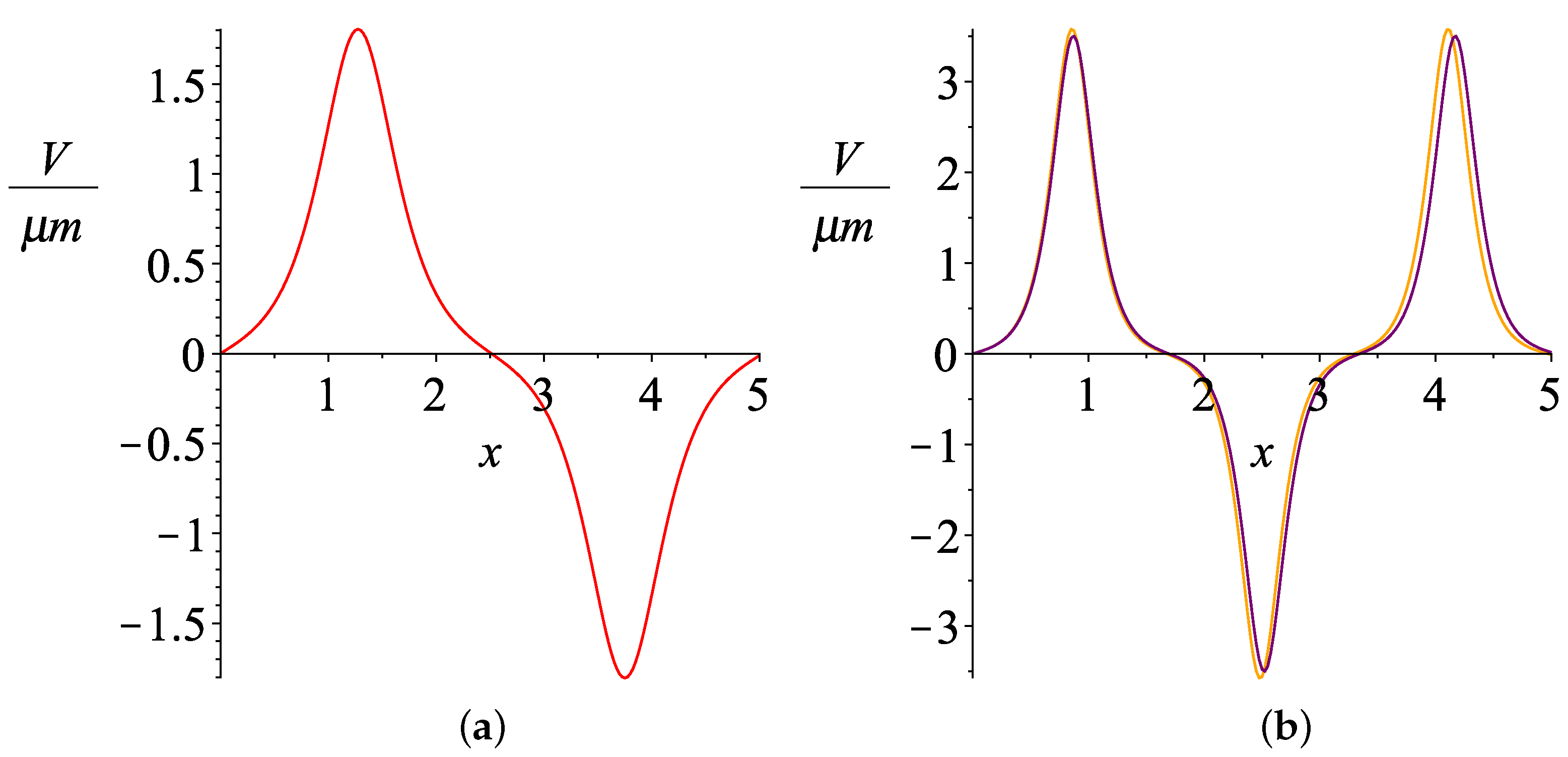
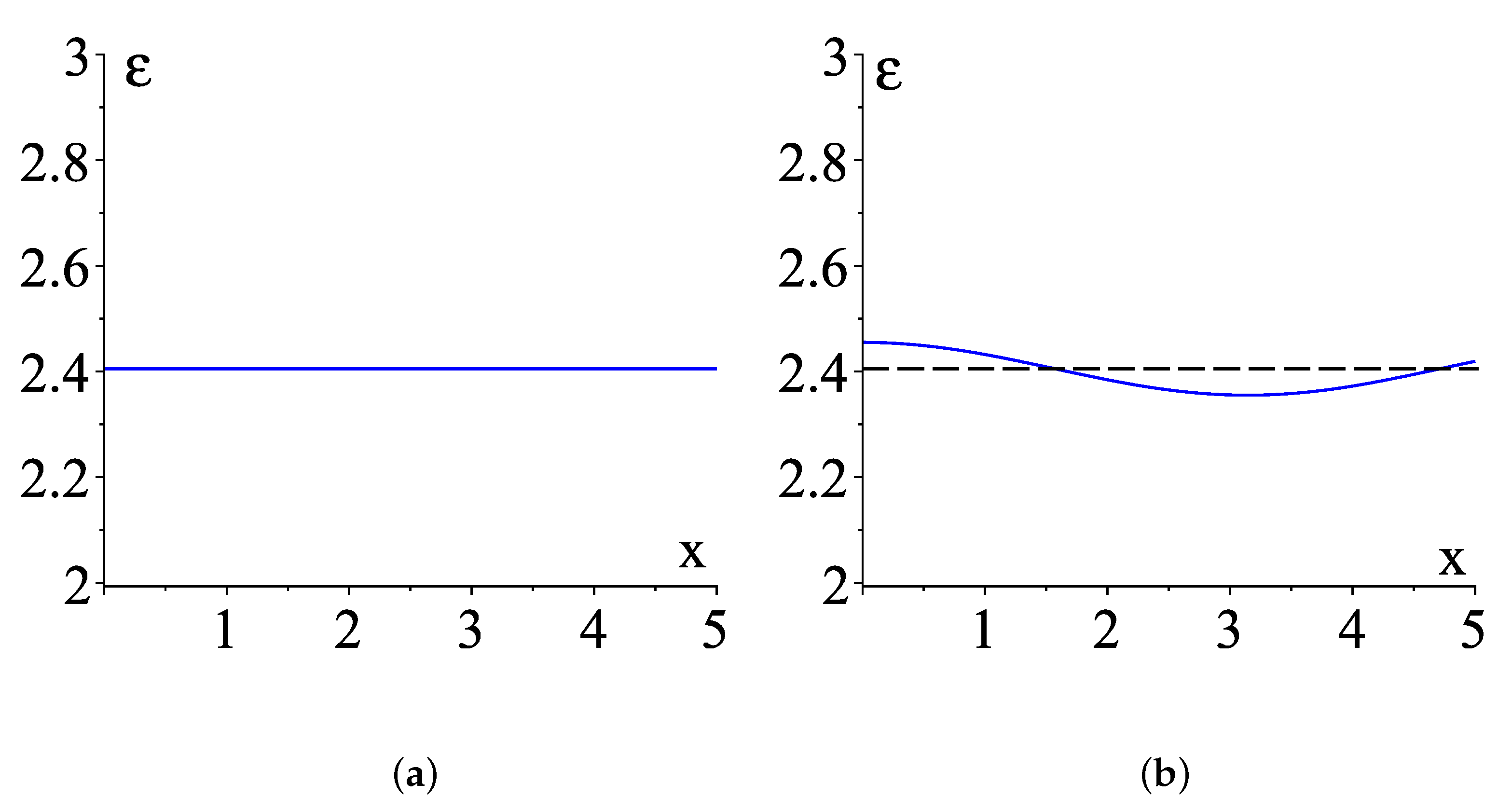
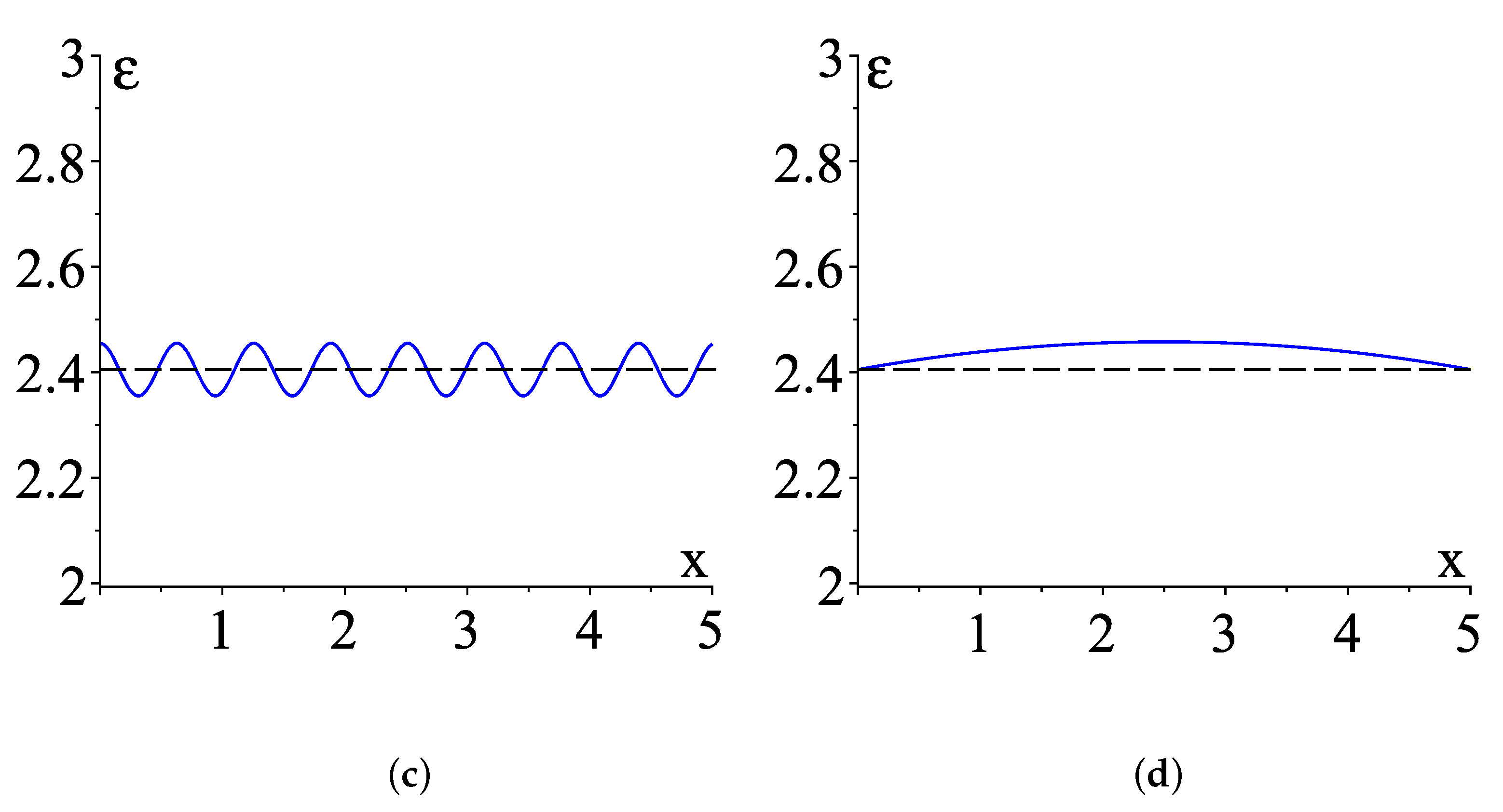
3.4. Numerical Results

In this section, we present some numerical results. In all calculations we used α = 6.4 × 10 12 m 2 / V 2 (except for the linear case where α always equals zero), ε 1 = 2.405 and A = 120 π · 10 3 V / m [28,29,30]; other parameters are given in the captions. Let us note that A is the value of u at the boundary x = 0 ; moreover, A is connected to the value of the z-th component of the magnetic field at the boundary x = 0 by the relationship
A = μ 0 ϵ 0 i H z ( 0 ) = 120 π i H z ( 0 ) .
In Figure 2, Figure 3, Figure 4, Figure 5, Figure 6, Figure 7, Figure 8, Figure 9, Figure 10 and Figure 11, we plot the dispersion curves (DCs) of problems P 0 , P 0 with β = 0 , P α and P . In these figures, only the first three DCs for each case are shown (this does not mean that there exist only three DCs in each case).
Generally speaking, DCs are plotted as the dependence of a wave number γ on either frequency ω of a wave or thickness h of a waveguide. Problems P 0 , P α , and P do not contain ω explicitly due to the normalization (7); for this reason, we plot DCs as γ vs h.
Please note that due to the normalization in the presented results, quantities γ and h are dimensionless; the real values of the wave number and width of the waveguide are k 0 γ and k 0 1 h , where k 0 is defined in (7).
The vertical black dashed line h = h * in Figure 2, Figure 3, Figure 4, Figure 5, Figure 6, Figure 7, Figure 8 and Figure 9 corresponds to a waveguide with fixed width k 0 1 h * . This line intersects DCs at some points denoted by solid diamonds; these points are propagation constants of the corresponding problem.
In nonlinear cases, it is possible that a few (different) propagation constants belong to the same DC. For this reason, to distinguish such propagation constants, we also use the notation γ ¯ n , m and γ ^ n , m for propagation constants of problems P α and P , respectively. In this notation, n = 1 , 2 , is a number of DC and m = 1 , 2 , is a number of the propagation constant among all eigenvalues that lie on the same DC and arranged in ascending order.
In Figure 2, DCs of problem P α and problem P 0 with β = 0 are shown. The brown diamonds denote the propagation constant γ ¯ 2 , 1 of problem P α ; this solution is close to the propagation constant γ ˜ 2 of problem P 0 with β = 0 denoted by the green diamond. Moreover, it can be shown that lim α + 0 γ ¯ 2 , 1 = γ ˜ 2 and the same is true about eigenmodes corresponding to these propagation constants. The blue diamond denotes propagation constant γ ¯ 2 , 2 of problem P α with no linear counterpart; this means that for any arbitrary small α solution, γ ¯ 2 , 2 does not tend to any propagation constant of the linear problem. Let us call such solutions purely nonlinear, meaning that they are not perturbations of linear solutions; these propagation constants correspond to novel eigenmodes of the waveguide. In Figure 10, there are eigenfunctions of problems P α and P 0 with β = 0 corresponding to the above-mentioned propagation constants.
Figure 12 shows the functions that we use to simulate perturbations of the linear part of the permittivity.
In Figure 3, Figure 5, Figure 7 and Figure 9, DCs of problem P and problem P α are shown. Theorem 2 assures that for sufficiently small values of parameter β , problem P has at least n solutions and each of them is located in some vicinity of the corresponding solution to problem P α . However, if | β | increases, then the numerical simulation produces unpredictable results. This means that the perturbed term is greatly affected if the perturbation is not sufficiently small (this is true at least for the range of parameters that we chose for the simulation). We do not present such figures as we cannot yet offer enough comment on this issue. In Figure 3, we demonstrate how the perturbed term presented in Figure 12, Subfigure (b) affects DCs.
We also note that pairs of DCs in the lower parts of Figure 3, Figure 5 and Figure 9 are very close to each other.

3.5. Proofs

3.5.1. Proof of Statement 4

The claim of Statement 4 is a direct consequence of the so-called integral continuous Theorem [27] applied to the Cauchy problem (8), (9) under the additional assumption about the global unique solvability of the Cauchy problem (11), (12) for x [ 0 , h ] , γ [ 0 , γ 0 ] , β ( β 0 , β 0 ) , and α ( 0 , α 0 ) . The validity of this additional assumption is guaranteed by Statement 2.

3.5.2. Proof of Statement 5

If γ = γ ^ is a propagation constant and u u ( x ; γ ^ , α , β ) is the corresponding eigenmode of problem P , then equality (19) is obviously satisfied.
Let u u ( x ; γ , α , β ) be a solution to a Cauchy problem (8), (9) and γ = γ * be a solution to equation u ( h ; γ , α , β ) = 0 . The only reason that can destroy our consideration is that there exists another solution u u * ( x ; γ * , α , β ) to the Cauchy problem (8), (9) and u u * for x [ 0 , h ] . However, this is not possible due to the classical result about the uniqueness of a solution to a Cauchy problem with some restrictions on the coefficients of the equation (these restrictions are satisfied for our equation). We stress that in this case, it is not important whether u * ( h ; γ * , α , β ) equals zero or not.

3.5.3. Proof of Statement 6

Statement 4 claims that the Cauchy problem (8), (9) is globally uniquely solvable and its solution u u ( x ; γ , β , α ) is defined and continuous for x [ 0 , h ] , γ [ 0 , γ 0 ] , β ( β 0 , β 0 ) , and α ( 0 , α 0 ) . Statement 2 claims that the Cauchy problem (11), (12) is globally uniquely solvable and its solution v v ( x ; γ , α ) is defined and continuous for x [ 0 , h ] , γ [ 0 , γ 0 ] , β ( β 0 , β 0 ) , and α ( 0 , α 0 ) . The fact that u ( x ; γ , β , α ) v ( x ; γ , α ) uniformly on x [ 0 , h ] and γ [ 0 , γ 0 ] as β 0 for any fixed α ( 0 , α 0 ) results from the integral continuous Theorem [27].

3.5.4. Proof of Theorem 2

Therefore, let γ 0 be sufficiently large that problem P α has n propagation constants γ ¯ k Γ , where k = 1 , k ¯ , such that for any γ ¯ k inequality (18) is satisfied.
Below, we need to use intervals Γ k = ( γ ¯ k δ k , γ ¯ k + δ k ) , where k = 1 , k ¯ and δ k > 0 are some constants, defined in Theorem 1. We note that Γ k does not contain other propagation constants except γ ¯ k for every k.
By virtue of Statement 6, the left-hand side of Equation (20) is bounded for γ [ 0 , γ 0 ] , β ( β 0 , β 0 ) for any fixed α ( 0 , α 0 ) and vanishes as β 0 .
Taking into account the above consideration, one comes to the conclusion that in any interval Γ k there exists γ ^ k satisfying Equation (20). Obviously, lim β 0 γ ^ k = γ ¯ k . In view of Statement 5 such γ ^ k is a propagation constant of problem P .

4. Discussion

In this paper, we studied the problem of monochromatic TE wave propagation in a plane-shielded waveguide filled with nonlinear nonhomogeneous medium with permittivity in the form (2). Such a model takes into account the presence of impurities in the medium causing slight deviations in the dielectric permittivity.
The main theoretical result of this study is Theorem 2. It states the existence of solutions (in particular, solutions without linear counterparts) to problem P .
We note that in accordance with Theorem 1, problem P α , which is a special case of problem P , has infinitely many propagation constants. In this regard, it is interesting to discover whether problem P has infinitely many propagation constants or not (there are at least two intriguing subcases: (a) β > 0 and (b) real β , where | β | is sufficiently small). However, the approach developed in the paper does not allow one to prove the existence of infinitely many solutions; see the comment just after Theorem 2.
It is also interesting to note that the influence of the small perturbation grows larger with the thickness of the waveguide and γ . This effect is readily seen in the upper part of Figure 3, in the right upper part of Figure 5, and in Figure 9 for the central part of the third DC. It is clear that the existence of infinitely many guided modes is impossible in any real physical system; however, it would be interesting to check experimentally whether at least a few first purely nonlinear solutions exist or not.
Despite the fact that absorption effects are some of the most important in any theory of wave propagation, we should say that it is not possible to include losses in the model under consideration. Indeed, the model under investigation in the paper was developed for a lossless film, i.e., the permittivity of the film is real [4,5,6]. Talking about the model, we mean the permittivity and the chosen type of fields. If the permittivity of the film has an imaginary part (which corresponds to the film with losses), then γ must be complex. However, this is impossible. Indeed, if γ is not real, then | e i γ z | depends on z and therefore the quantity | E | 2 = | E y ( x ) e i γ z | 2 also depends on z; see Formulas (1) or (2). This contradicts the choice of the field components in the form (3). The problem of finding complex guided modes in the nonlinear regime is a nontrivial one.

Author Contributions

Methodology, D.V.; software, A.D.; investigation, A.D. and S.T.; writing—original draft preparation, A.D. and S.T.; writing—review and editing, D.V.; visualization, A.D.; supervision, D.V. All authors have read and agreed to the published version of the manuscript.

Funding

The research was funded by the Russian Science Foundation under the project 18-71-10015.

Institutional Review Board Statement

Not applicable.

Informed Consent Statement

Not applicable.

Data Availability Statement

Not applicable.

Acknowledgments

We thank the anonymous referees whose comments and remarks helped us to improve the paper.

Conflicts of Interest

The authors declare no conflict of interest.

References

  1. Unger, H.G. Planar Optical Waveguides and Fibres; Clarendon Press: Oxford, UK, 1977. [Google Scholar]
  2. Snyder, A.; Love, J. Optical Waveguide Theory; Chapman and Hall: London, UK, 1983. [Google Scholar]
  3. Sodha, M.S.; Ghatak, A.K. Inhomogeneous Optical Waveguides; Optical Physics and Engineering; Plenum Press: New York, NY, USA; London, UK, 1977. [Google Scholar]
  4. Landau, L.D.; Lifshitz, E.M.; Pitaevskii, L.P. Course of Theoretical Physics (vol.8). Electrodynamics of Continuous Media; Butterworth-Heinemann: Oxford, UK, 1993. [Google Scholar]
  5. Akhmediev, N.N.; Ankevich, A. Solitons, Nonlinear Pulses and Beams; Chapman and Hall: London, UK, 1997. [Google Scholar]
  6. Boardman, A.D.; Egan, P.; Lederer, F.; Langbein, U.; Mihalache, D. Third-Order Nonlinear Electromagnetic TE and TM Guided Waves. In Nonlinear Surface Electromagnetic Phenomena; Ponath, H.-E., Stegeman, G.I., Eds.; Elsevier Science Publisher: North-Holland, The Amsterdam; London, UK; New York, NY, USA; Tokyo, Japan, 1991. [Google Scholar]
  7. Boyd, R.W. Nonlinear Optics, 2nd ed.; Academic Press: New York, NY, USA; London, UK, 2003. [Google Scholar]
  8. Mills, D.L. Nonlinear Optics: Basic Concepts; Springer: Berlin/Heidelberg, Germany, 1991. [Google Scholar]
  9. Zakery, A.; Elliott, S.R. Optical Nonlinearities in Chalcogenide Glasses and Their Applications; Springer Series in Optical Sciences; Springer: Berlin/Heidelberg, Germany, 2007; Volume 135. [Google Scholar]
  10. Li, C. Nonlinear Optics Principles and Applications; Shanghai Jiao Tong University Press: Shanghai, China; Springer: Berlin/Heidelberg, Germany, 2015. [Google Scholar]
  11. Khoo, I.C. Nonlinear optics, active plasmonics and metamaterials with liquid crystals. Prog. Quantum Electron. 2014, 38, 77–117. [Google Scholar] [CrossRef]
  12. Borghi, M.; Castellan, C.; Signorini, S.; Trenti, A.; Pavesi, L. Nonlinear silicon photonics. J. Opt. 2017, 19, 093002. [Google Scholar] [CrossRef]
  13. Schürmann, H.W. On the theory of TE-polarized waves guided by a nonlinear three-layer structure. Z. Phys. B 1995, 97, 515–522. [Google Scholar] [CrossRef]
  14. Smirnov, Y.G.; Valovik, D.V. Guided electromagnetic waves propagating in a plane dielectric waveguide with nonlinear permittivity. Phys. Rev. A 2015, 91, 013840. [Google Scholar] [CrossRef]
  15. Valovik, D.V. Novel propagation regimes for TE waves guided by a waveguide filled with Kerr medium. J. Nonlinear Opt. Phys. Mater. 2016, 25, 1650051. [Google Scholar] [CrossRef]
  16. Said, A.A.; Wamsley, C.; Hagan, D.J.; Stryland, E.W.V.; Reinhardt, B.A.; Roderer, P.; Dillard, A.G. Third- and fifth-order optical nonlinearities in organic materials. Chem. Phys. Lett. 1994, 228, 646–650. [Google Scholar] [CrossRef]
  17. Tan, C.; Li, N.; Xu, D.; Chen, Z. Spatial focusing of surface polaritons based on cross-phase modulation. Results Phys. 2021, 27, 104531. [Google Scholar] [CrossRef]
  18. Schürmann, H.W.; Smirnov, Y.G.; Shestopalov, Y.V. Propagation of TE-waves in Cylindrical Nonlinear Dielectric Waveguides. Phys. Rev. E 2005, 71, 016614. [Google Scholar] [CrossRef] [PubMed]
  19. Smirnov, Y.G.; Valovik, D.V. Coupled Electromagnetic TE-TM Wave Propagation in a Layer with Kerr Nonlinearity. J. Math. Phys. 2012, 53, 123530. [Google Scholar] [CrossRef]
  20. Valovik, D.V. Nonlinear multi-frequency electromagnetic wave propagation phenomena. J. Opt. 2017, 19, 115502. [Google Scholar] [CrossRef]
  21. Valovik, D.V. On a nonlinear eigenvalue problem related to the theory of propagation of electromagnetic waves. Differ. Equ. 2018, 54, 168–179. [Google Scholar] [CrossRef]
  22. Valovik, D.V. On spectral properties of the Sturm–Liouville operator with power nonlinearity. Monatshefte Math. 2019, 188, 369–385. [Google Scholar] [CrossRef]
  23. Moskaleva, M.A.; Kurseeva, V.Y.; Valovik, D.V. Asymptotical analysis of a nonlinear Sturm–Liouville problem: Linearisable and non-linearisable solutions. Asymptot. Anal. 2020, 119, 39–59. [Google Scholar]
  24. Adams, M.J. An Introduction to Optical Waveguides; John Wiley & Sons: Chichester, UK; New York, NY, USA; Brisbane, Australia; Toronto, ON, Canada, 1981. [Google Scholar]
  25. Marcuse, D. Theory of Dielectric Optical Waveguides, 2nd ed.; Academic Press: Cambridge, MA, USA, 1991. [Google Scholar]
  26. Courant, R.; Hilbert, D. Methods of Mathematical Physics; Interscience Publishers Inc.: New York, NY, USA, 1953; Volume 1. [Google Scholar]
  27. Pontryagin, L.S. Ordinary Differential Equations; Pergamon Press: Oxford, UK, 1962. [Google Scholar]
  28. Mihalache, D.; Stegeman, G.I.; Seaton, C.T.; Wright, E.M.; Zanoni, R.; Boardman, A.D.; Twardowki, T. Exact dispersion relations for transverse magnetic polarized guided waves at a nonlinear interface. Opt. Lett. 1987, 12, 187–189. [Google Scholar] [CrossRef] [PubMed]
  29. Chen, Q.; Wang, Z.H. Exact dispersion relations for TM waves guided by thin dielectrics films bounded by nonlinear media. Opt. Lett. 1993, 18, 260–262. [Google Scholar] [CrossRef] [PubMed]
  30. Huang, J.H.; Chang, R.; Leung, P.T.; Tsai, D.P. Nonlinear dispersion relation for surface plasmon at a metal-Kerr medium interface. Opt. Commun. 2009, 282, 1412–1415. [Google Scholar] [CrossRef]
Figure 1. Geometry of the problem.
Photonics 10 00371 g001
Figure 2. Dispersion curves of problem P α (blue curve) and problem P 0 with β = 0 (red curve). Solid diamonds denote the propagation constants γ ˜ 1 1.415 (red), γ ˜ 2 0.902 (green) of problem P 0 with β = 0 and propagation constants γ ¯ 2 , 1 1.141 (brown), γ ¯ 2 , 2 3.705 (blue) of problem P α .
Photonics 10 00371 g002
Figure 3. Dispersion curves of problem P α (blue curve) with ε = 2.405 and problem P α β (green curve) with ε = 2.405 + 0.05 cos ( x ) . Solid diamonds denote the propagation constants γ ¯ 2 , 1 1.141 (blue), γ ¯ 2 , 2 3.705 (orange) of problem P α and propagation constants γ ^ 2 , 1 1.131 (green), γ ^ 2 , 2 4.197 (purple) of problem P α β .
Photonics 10 00371 g003
Figure 4. Subfigure (a): the eigenfunction of problem P α β (green curve) corresponding to the propagation constant denoted by the green diamond in Figure 3. Subfigure (b): the eigenmodes of problems P α β (purple curve) and P α (orange curve) corresponding to the propagation constants denoted by the purple and orange diamonds in Figure 3.
Photonics 10 00371 g004
Figure 5. Dispersion curves of problem P α (blue curve) with ε = 2.405 and problem P α β (green curve) with ε = 2.405 + 0.05 cos ( 10 x ) . Solid diamonds denote propagation constants γ ¯ 2 , 1 1.141 (blue), γ ¯ 2 , 2 3.705 (orange) of problem P α and propagation constants γ ^ 2 , 1 1.115 (green), γ ^ 2 , 2 3.656 (purple) of problem P α β .
Photonics 10 00371 g005
Figure 6. Subfigure (a): the eigenmode of problem P α β (green curve) corresponding to the propagation constant denoted by the green diamonds in Figure 5. Subfigure (b): the eigenmode of problem P α β (purple curve) corresponding to the propagation constant denoted by the purple diamonds in Figure 5.
Photonics 10 00371 g006
Figure 7. Dispersion curves of problem P α (blue curve) with ε = 2.405 and problem P α β (green curve) with ε = 2.405 + 0.05 cos ( 4 x ) . Solid diamonds denote propagation constants γ ¯ 2 , 1 1.141 (blue), γ ¯ 2 , 2 3.705 (orange) of problem P α and propagation constants γ ^ 2 , 1 1.112 (green), γ ^ 2 , 2 3.404 (purple) of problem P α β .
Photonics 10 00371 g007
Figure 8. Subfigure (a): the eigenmode of problem P α β (green curve) corresponding to the propagation constant denoted by the green diamond in Figure 7. Subfigure (b): the eigenmode of problem P α β (purple curve) and P α (orange curve) corresponding to the propagation constant denoted by the purple and orange diamonds in Figure 7.
Photonics 10 00371 g008
Figure 9. Dispersion curves of problem P α (blue curve) with ε = 2.405 and problem P α β (green curve) with ε = 2.405 + 0.00526 ( 1.6 x 2 + 8 x ) . Solid diamonds denote propagation constants γ ¯ 2 , 1 1.141 (blue), γ ¯ 2 , 2 3.705 (brown), γ ¯ 3 , 1 6.866 (orange) of problem P α and propagation constants γ ^ 2 , 1 1.179 (green), γ ^ 2 , 2 3.585 (red), γ ^ 3 , 1 6.493 (purple) of problem P α β .
Photonics 10 00371 g009
Figure 10. Subfigure (a): the eigenfunctions of problem P α (brown curve) and problem P 0 with β = 0 (green curve) corresponding to the propagation constants denoted by the green and brown diamonds in Figure 2. Subfigure (b): the eigenfunction corresponding to the propagation constant of problem P α denoted by the blue diamonds in Figure 2.
Photonics 10 00371 g010
Figure 11. Subfigure (a): the eigenmode of problem P α β (red curve) corresponding to the propagation constant denoted by the red diamonds in Figure 9. Subfigure (b): the eigenmodes of problems P α β (purple curve) and P α (orange curve) corresponding to the propagation constants denoted by the purple and orange diamonds in Figure 9.
Photonics 10 00371 g011
Figure 12. In subfigure (a) ε = 2.405 , in subfigure (b) ε = 2.405 + 0.05 cos ( x ) , in subfigure (c) ε = 2.405 + 0.05 cos ( 10 x ) , in subfigure (d) ε = 2.405 + 0.00526 ( 1.6 x 2 + 8 x ) .
Photonics 10 00371 g012aPhotonics 10 00371 g012b
Disclaimer/Publisher’s Note: The statements, opinions and data contained in all publications are solely those of the individual author(s) and contributor(s) and not of MDPI and/or the editor(s). MDPI and/or the editor(s) disclaim responsibility for any injury to people or property resulting from any ideas, methods, instructions or products referred to in the content.

