1. Introduction
For high-power laser facilities, the wavefront distribution is an important factor that affects the laser driver’s focal spot characteristics, which is severely affected by the transmitted wavefronts of the total optics of whole systems. In many high-power laser facilities, such as the National Ignition Facility (NIF) [
1,
2,
3,
4], Laser Megajoule (LMJ) [
5,
6,
7], and Shenguang-II Upgrade (SG-II UP) [
8,
9,
10] and Shenguang-III (SG-III) [
11], pulses propagate through the multipass optical paths of booster amplifiers and cavity amplifiers, enter the final optics assembly (FOA), and finally shoot on the target. Many large-aperture optical elements exist in the complex chains of a facility, such as Nd:glass slabs, spatial filter systems, focusing elements in FOA, and debris shields. They all have different transmitted wavefronts because of the machining precision, pressure distortion during installation, and the effect of the environment. The lasers inevitably carry wavefront errors when propagating through the system. As a result, they affect the quality of the focal spot and decrease the focal energy concentration and focusing power density. This is unfavorable for physics experiments with high-power lasers.
The focal spot quality of laser drivers is mainly determined by the output wavefront error introduced by large-diameter optics [
12]. In these facilities, the output beam, although being an input with a uniform wavefront, will have wavefront errors with spatial wavelengths ranging from a few centimeters to several hundred nanometers [
13,
14]. The wavefront peak-to-valley (PV) value, wavefront root-mean-squared gradient (GRMS), and power spectral density (PSD) have been used to evaluate beam wavefront errors. The spatial frequency [
11,
12,
13,
14,
15,
16] is divided into four types: low spatial frequency (
v < 0.0303 mm
−1), mid-1 spatial frequency (PSD-1:0.0303–0.4 mm
−1), mid-2 spatial frequency (PSD-2:0.4–8.33 mm
−1), and high spatial frequency
(v > 8.33 mm
−1). Among them, a low-spatial-frequency wavefront error is mainly affected by the spherical aberration, coma, and astigmatism of optics, which is usually analyzed via GRMS. A mid-spatial-frequency wavefront error, also called a waviness error, can easily induce intensity modulation and self-focusing effects and damage the elements during transmission. PSD is effective for analyzing mid-spatial-frequency wavefront errors. A high-spatial-frequency wavefront error mainly refers to roughness, which is usually characterized via the roughness root mean square (RMS) value and is often filtered out by the spatial filter system. The wavefront PV value is typically used to roughly characterize the beam wavefront errors.
Wavefront errors can degenerate the quality of the focal spot, and several reports have studied the influence of wavefront errors on the far-field characteristics of high-power laser drivers [
11,
12,
13,
14,
15,
16,
17]. However, most of them only give the element machining requirements via a wavefront error for a single optical element. Few have considered systematic accumulated wavefronts with respect to the whole layout of a facility. The output wavefront in the FOA is difficult to simulate precisely because of various factors such as installation pressure by clamping, thermal distortion by pumping, and the deformable mirror in the adaptive optical (AO) system. In this paper, we investigated wavefronts of large-diameter beams, which were predicted by realistic transmitted wavefronts of Nd:glass slabs, debris shields, and the systematic accumulated static wavefront. Based on the layout of the SG-II UP facility, the wavefronts were divided into different spatial frequency types by PSD wavefront frequency bands, and the influence of each type on the focal spot characteristics was quantitatively analyzed. The results are expected to provide the allowable PV value range of the wavefront errors, which can be used to improve the quality of focal spots by the AO system and guide the processing of large-aperture optics. In addition, for high-power laser facilities, a focal spot on a target is difficult to measure due to the extremely high power density. This study is also beneficial to the prediction of focal spots according to the acquired data of the wavefront.
A wavefront error will cause the modulation of the near and far fields of a beam during the propagation, meaning the characteristics of the focal spot will be affected.
Section 2 of this paper presents the theoretical model, the layout of the SG-II UP facility, and machine surface characteristics of large-diameter optics. The transmitted wavefront is given by the machine surface characteristics and is divided by the PSD band.
Section 3 investigates the influence on the focal spot, focal shape, energy concentration, Strehl ratio, and relative intensity of sidelobes. Accordingly, the allowable wavefront PV value of the optics and the direction of optimization are provided. Finally, a conclusion is drawn in
Section 4.
2. Theoretical Model
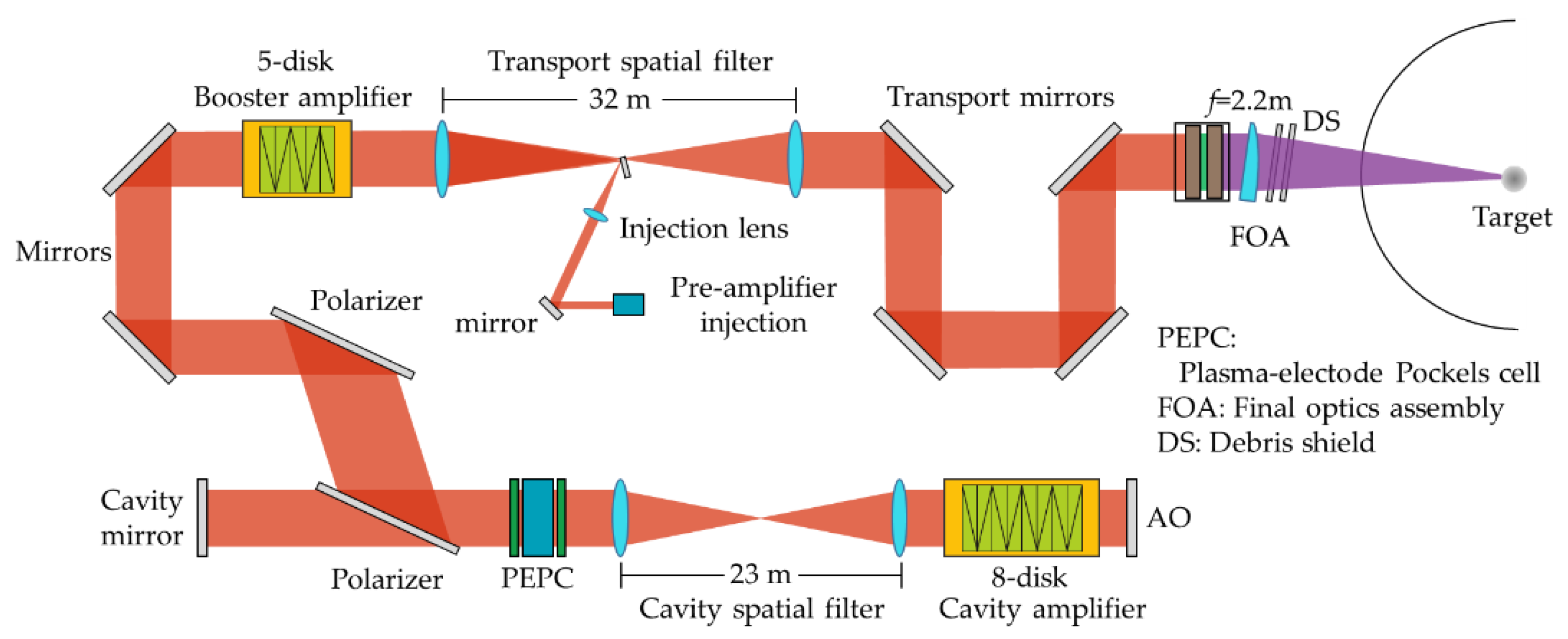
The layout of the SG-II UP facility is shown in
Figure 1. The beam is injected into the main amplification chain by a pre-amplifier, propagates through a two-pass booster amplifier and four-pass cavity amplifier, and finally enters the FOA. In the SG-II UP facility, the booster amplifier and cavity amplifier are composed of five and eight pieces of Nd:glass slabs, respectively. After the beam enters the amplification system, it will pass through 42 Nd:glass slabs and at least one debris shield, and then shoot at the target. Additionally, the Hartmann sensor is placed between the output of the transport spatial filter and the injection of FOA to measure the beam wavefront for the correction of the adaptive optics system.
The actual output wavefront in the FOA is difficult to simulate accurately. Additionally, it can only be predicted with the static wavefront of the elements measured by an interferometer or AO system. To deduce a beam wavefront via the optics-transmitted wavefront, fortunately, the processing wavefront of the elements is often similar, and the wavefront errors introduced by the installation and pump are mainly low-spatial-frequency errors. Therefore, when predicting the output laser wavefront in the structure of
Figure 1, two methods were selected in this study: one relies on the transmitted wavefronts of optics which has high similarity, such as Nd:glass slabs and debris shields, and the other relies on accumulating the static wavefronts of optics in the chain of the SG-II UP facility.
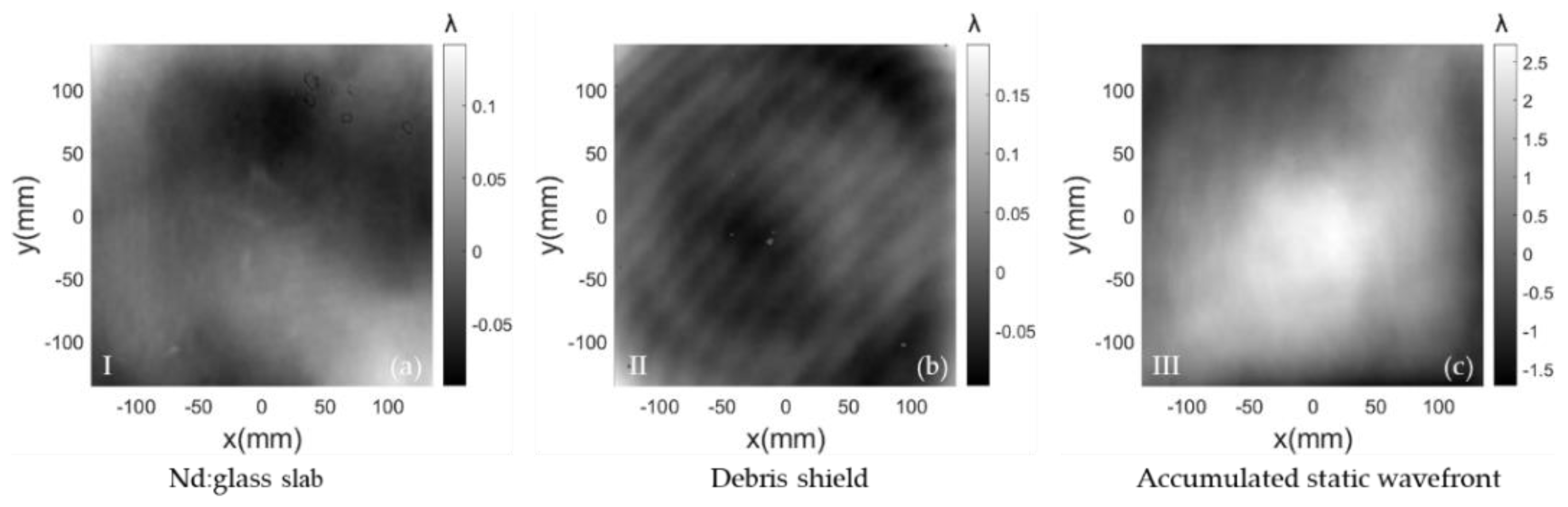
Generally, the average PV of a Nd:glass wavefront is approximately 0.25
λ. A measured transmitted wavefront distribution of Nd:glass, which changes slowly without obvious periodic modulation, is displayed in
Figure 2a and numbered I. The SG-II UP facility consists of eight beamlets, and the one we chose in our study contains 13 Nd:glass slabs, and the PV values of them are 0.25
λ, 0.25
λ, 0.21
λ, 0.26
λ, 0.28
λ, 0.30
λ, 0.27
λ, 0.38
λ, 0.22
λ, 0.65
λ, 0.14
λ, 0.24
λ, and 0.31
λ.
The transmitted wavefront PV of the debris shield in SG-II UP is generally between 0.3
λ and 0.5
λ. A measured transmitted wavefront is shown in
Figure 2b and numbered II, which carries rings with periodic stripe phase modulation.
An accumulated static wavefront, shown in
Figure 2c and numbered III, was achieved by superposing all the measured transmitted wavefronts of the large-aperture elements according to the layout of the SG-II UP facility. The PV value reached 4.45
λ. The accumulated wavefront was smoother, and the stripes introduced by a single debris shield were inconspicuous.
We used these transmitted wavefronts and accumulated wavefronts as the predicted ones of the beam to analyze the influence of these three types of wavefronts on the focal spot.
The Holaser software [
18,
19], a self-developed software and formerly called the Laser designer, was used in the theoretical calculations. It is employed for the design and improvement of SG-II UP systems, and its validity has been proven experimentally. The software used the beam diffraction propagation method based on physical field tracing to calculate the output focal spot. The calculation formula used was as follows:
where
n0 and
n2 are the linear refractive index and nonlinear refractive coefficient of the medium, respectively, and
k0 is the wavenumber
. The first two terms represent the diffraction effect, and the third represents the nonlinear self-focusing effect. Equation (1) can be solved using the Split-step Fourier method [
20]. To study the influence of the wavefront on the focal spot, the nonlinear transmission is not analyzed in the calculation.
In addition, to improve the resolution of the focal spot calculation, the Fresnel diffraction we used was:
where (
x0,
y0) and (
x,
y) are the points on the diffraction and observation screens, respectively.
The output of the SG-II UP system was a square beam with dimensions of 310 mm × 310 mm. In our calculation, it was assumed to be an ideal super-Gaussian profile, described as:
where
A0 is the signal amplitude;
nx and
ny represent the spatial distribution of the laser pulse in the
x and
y directions, respectively (
nx,
ny >1 is a super-Gaussian beam);
ax and
ay are the half-width at half maximum for the spatial distribution of a pulse in the
x- and
y-directions, respectively; and
is the output beam wavefront, predicted based on the optical path arrangement and large-diameter optical components.
To evaluate the wavefront of a SG-II UP system with respect to the PSD, it is necessary to solve and filter the wavefront distribution of the output beam. In this study, the least squares method [
21,
22] was used, and the solution was obtained using the discrete cosine transform. The wavefront information in different bands was obtained via the filtered wavefront according to the PSD requirements.
The filtering process is performed as follows [
12]: First, a Fourier transform on
is performed to obtain the wavefront spectrum
:
The wavefront spectrum
is then filtered by
, which is a low-pass function, a band-pass function, or a high-pass function in different calculation situations.
Finally, inverse Fourier transform is performed on
to obtain the filtered wavefront phase.
The 10th-order Gaussian distribution function was used as the filtering function in this study and was substituted into Equation (3). Equations (1) and (2) were then used to calculate along the propagation optical path of the FOA, and finally, the distribution of the focal spot of the large-diameter laser could be obtained.
The energy concentration (
Ec), Strehl ratio (SR), and sidelobe relative intensity were used to evaluate the quality of the focal spot.
Ec is described as [
23]:
If Ec is larger, the energy on the focal spot is more concentrated, and the quality of the focal spot is better than that of the smaller value at the same focal spot size.
The Strehl ratio is the ratio of the actual far-field peak intensity along the beam axis to the peak light intensity of an ideal beam with the same amplitude distribution and a uniform phase, given by [
24]:
where
A(
x,
y) represents the actual amplitude distribution of the beam, and
is the phase distribution. Generally, a higher SR indicates a higher peak intensity for the focal spot.
The relative intensity of the focal spot sidelobes is defined as the ratio of the focal spot sidelobe intensity to the peak intensity. This is related to the power density of the focal sidelobe. The greater the relative intensity, the higher the possibility that hole-blocking occurs in the spatial filter system in the chain.
The transmitted wavefront is segmented by a PSD wavefront frequency band. By changing the wavefront PV value of the segmentation, its effect on the focal spot could be evaluated in this study.
3. Numerical Calculation and Analysis Results
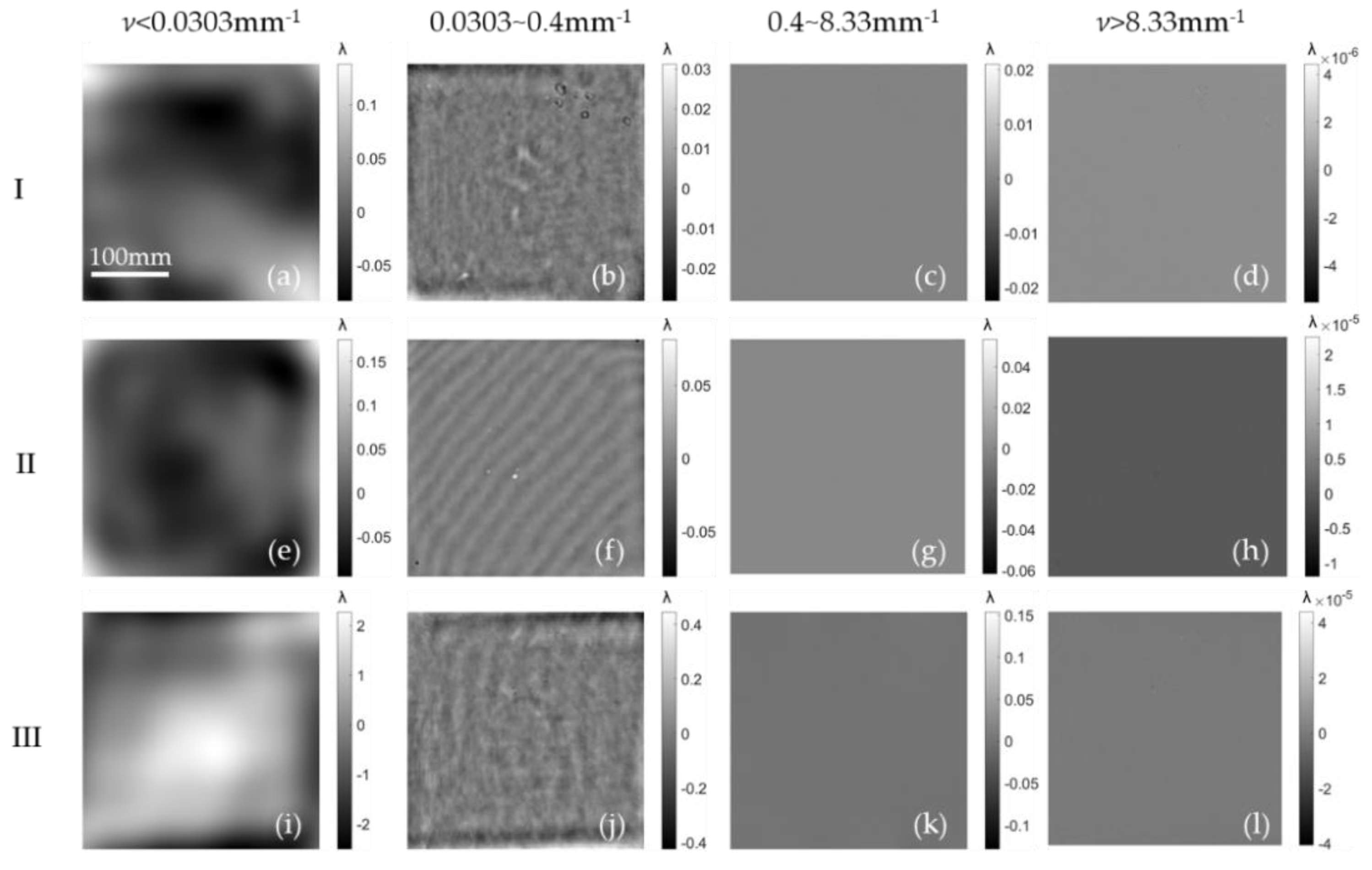
According to
Section 2, the transmitted wavefront of the Nd:glass, the debris shield, and static wavefront, recorded as wavefront I, II, and III, respectively, are typically used as the three typical wavefronts of the output beam in FOA. They are used to simulate the output wavefront of the facility as the original wavefronts. According to the PSD band, the original wavefronts are divided into low spatial frequency:
ν < 0.0303 mm
−1, PSD-1: 0.0303–0.4 mm
−1, PSD-2: 0.4–8.33 mm
−1; and high spatial frequency:
ν > 8.33 mm
−1; the filtered wavefronts are shown as depicted in
Figure 3. The distributions of the low spatial frequency (column 1) and the PSD-1 (column 2) are different. However, the high spatial frequency (column 4) is limited by the resolution of the ZYGO interferometer, and it is mostly noise from the measurement process and will not represent the real high-spatial-frequency distribution; therefore, it is not discussed and analyzed in this paper.
We normalized the wavefront PV value. When the PV values of the original wavefronts are 1
λ, and the PV value ratio of each filtered wavefront part is maintained, the PV values of the filtered wavefront are listed in
Table 1. From
Table 1, for the PV values of the low-spatial-frequency type, the largest is wavefront III, while the lowest is II; for the mid-spatial-frequency type, the results are the opposite. This indicates that the accumulated wavefront, wavefront III, has certain complementarity in the mid-frequency types, which is beneficial for a more uniform and smoother wavefront distribution. The following section quantitatively analyzes the effect of different wavefront types on the focal spot characteristics by varying the PV values.
3.1. Shape of Focal Spot
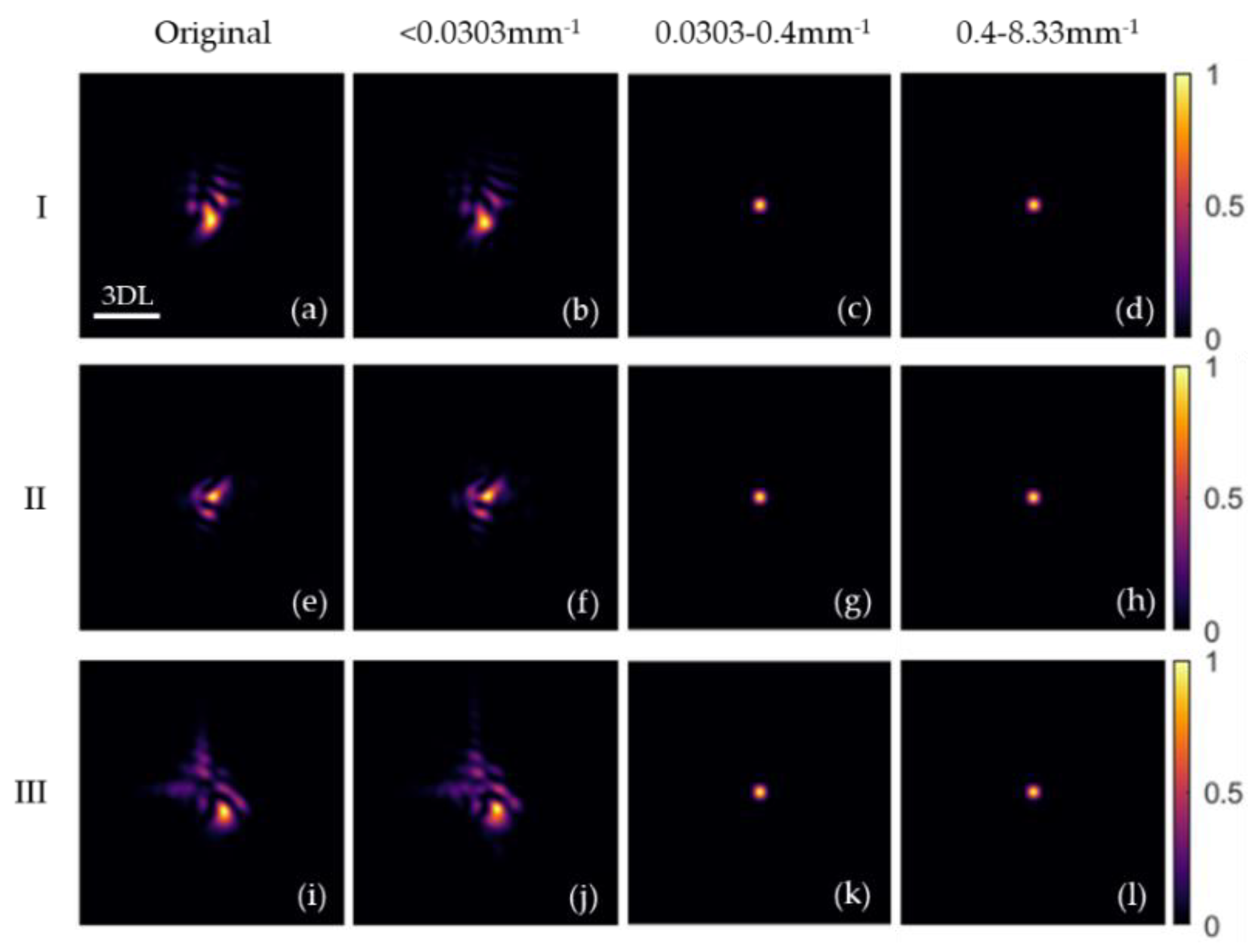
The three original wavefronts in
Figure 2 and the filtered wavefront of the low-spatial-frequency, PSD-1, and PSD-2 parts in
Figure 3 were considered as the beam wavefront. The far-field focal spots of these wavefronts are shown in
Figure 4, where all the PV values of the different spatial frequency types are equal to 2λ for an obvious comparison, which were calculated with the parameters of the FOA in the SG-II UP facility [
25].
In
Figure 4, rows 1–3 present the focal spots corresponding to wavefronts I, II, and III, respectively. Column 1 shows the focal profiles of the unfiltered original wavefront distribution, and column 2 shows the focal profiles of the low-spatial-frequency wavefront. Columns 3 and 4 represent the focal profiles of PSD-1 and PSD-2, respectively. Additionally, 3DL is a scale bar, which means 3 times the diffraction limit (DL). The one-dimensional relative intensity distributions of the focal spot are shown in
Figure 5, obtained by the focal profiles of the centers in
Figure 4.
Two features can be obtained from
Figure 4 and
Figure 5. First, when different wavefronts have the same PV value, the focal spot of the low spatial frequency is roughly similar to the original wavefront in the three cases, which has a similar profile and dispersion. Second, there is no apparent dispersion or splitting in the focal spot of the mid-spatial-frequency band. Therefore, it can be concluded that the focal profile is mainly determined by the low-spatial-frequency wavefront.
3.2. Energy Concentration of Focal Spot
Energy concentration (Ec) is an important parameter to evaluate the effecient energy of the focal spot in the field of high-power lasers. Moreover, the Ec is closely related to the dispersion of the focal spot. The relationship between Ec and the wavefront distribution is of great significance for facility optimization.
The low spatial frequency (<0.0303 mm
−1), low spatial frequency + PSD-1 (<0.4 mm
−1), low spatial frequency + PSD-1 + PSD-2 (<8.33 mm
−1), and ideal wavefront of I, II, and III were used as the calculation wavefronts of the beam, and the focal spot distribution was calculated to obtain the
Ec of the focal spot, as shown in
Figure 6, where the original wavefront PV = 2
λ and the PV value ratio of each filtered wavefront was maintained and unchanged. Here, the gray, blue, red, and green curves represent the
Ec of the low spatial frequency, low spatial frequency + PSD-1, low spatial frequency + PSD-1 + PSD-2, and the ideal beam without wavefront errors, respectively.
The gray, blue, and red curves have similar change trends, far worse than the green curve under the same focal size. The red and blue curves almost coincide. These results indicate that Ec is mainly determined by the low-spatial-frequency wavefront, and the PSD-2 has almost no effect on Ec. Therefore, to obtain a high Ec of the focal spot, the low-spatial-frequency wavefront error should be focused on during AO correction in the future.
In high-power laser facilities, energy concentration within 3 DL (
Ec3DL) and 10DL (
Ec10DL) is usually focused on when evaluating the quality of the focal spot. The
Ec3DL/
Ec10DL variations in each spatial-frequency part with the original wavefront PV value are given in
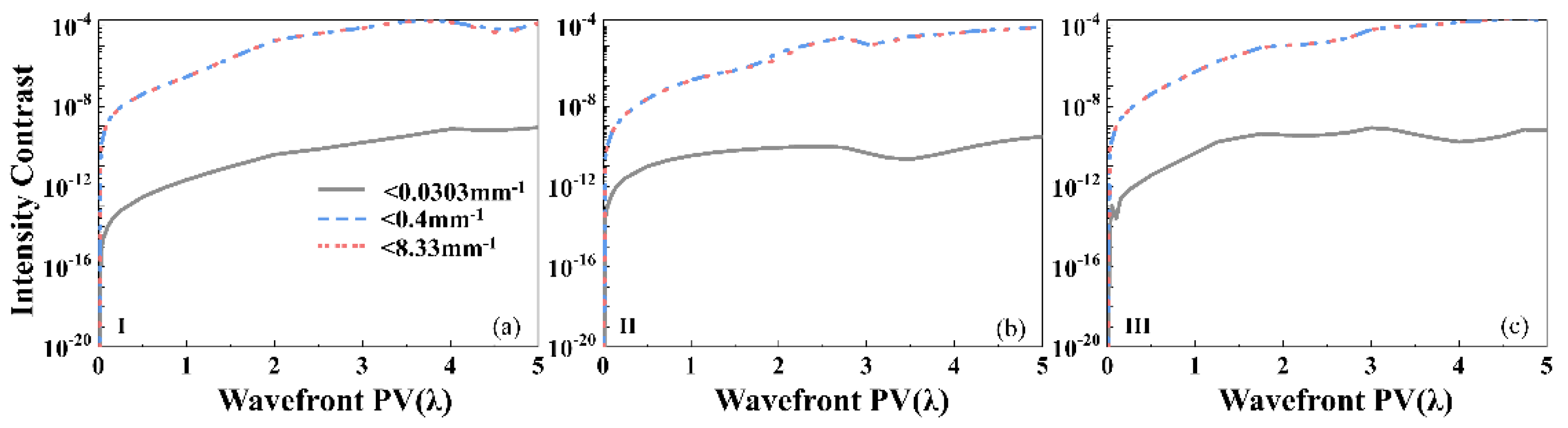
Figure 7.
Figure 7a–c display the changes in
Ec3DL of wavefront I, II, and III, while
Figure 7d–f present the changes in
Ec10DL. In each figure, the gray, blue, and red curves represent the
Ec of the low-spatial-frequency wavefront (<0.0303 mm
−1), the low-spatial-frequency + PSD-1 part (<0.4 mm
−1), and the low-spatial-frequency + PSD-1 + PSD-2 part (<8.33 mm
−1), respectively.
In
Figure 7, the overlap of the curves between <0.4 mm
−1 and <8.33 mm
−1 indicates that
Ec is less affected by the PSD-2 wavefront. Additionally, the separation of the curves between <0.4 mm
−1 and <0.0303 mm
−1 indicates that PSD-1 has some influence on
Ec. When the original wavefront PV reached 2
λ, the
Ec3DL of wavefronts I, II, and III were calculated as 76.9%, 81.5%, and 61.3%, respectively, while the
Ec10DL of wavefronts I, II, and III were 98.9%, 96.8%, and 98.2%, respectively. This demonstrates that wavefront III has a significant influence on
Ec3DL, while wavefront II has a significant influence on
Ec10DL.
In particular, if
Ec3DL ≥ 50% or
Ec3DL ≥ 95% is required in the SG-II UP facility, the maximum allowable PV values are provided in
Table 2, according to
Figure 7.
Table 2 shows the maximum allowable PV values of the original wavefront when
Ec3DL = 50% and
Ec10DL = 95% under low- and full-spatial-frequency wavefronts. For
Ec3DL = 50%, the discrepancy of PV value between the low-spatial-frequency type and full spatial frequency is very small, which indicates the mid-spatial-frequency type has a weak influence. However, for
Ec10DL = 95%, the effect of the mid-spatial-frequency wavefront is significant and cannot be neglected. Particularly, because of wavefront II with periodic modulation in PSD-1, as shown in
Figure 3f, its discrepancy is up to 2.09
λ when
Ec10DL = 95%. Therefore, to obtain high energy concentration, it is necessary to avoid a periodic wavefront error in the FOA beam.
In addition, as shown in
Table 2, for the three types of wavefronts, the requirements of
Ec3DL = 50% and
Ec10DL = 95% are not equivalent. Wavefront III has the smallest differences in allowable PV values between the two requirements, whereas wavefront II has the largest. Furthermore, if there are no periodic modulations in the laser wavefront, the allowable PV value of the two requirements is generally less than 0.5
λ, and
Ec3DL ≥ 50% is a more rigorous requirement.
For the three typical wavefronts in this study, if Ec3DL ≥ 50% or Ec10DL ≥ 95% is required, the wavefront PV value of the output laser in FOA must not exceed 2.27λ and 2.45λ, respectively.
3.3. Strehl Ratio of Focal Spot
The wavefronts of different spatial-frequency types of I, II, and III were used as the calculated wavefronts, as in
Section 3.2, and the variations in their SRs with the PV value of the original wavefront are shown in
Figure 8.
Figure 8a shows the SR variations in wavefront I with different spatial-frequency types, and the three SR curves almost overlap. This indicates that the SR is almost affected by the low spatial frequency. There are similar changes to the SRs of wavefront II and III.
Figure 8b compares the SRs of the wavefront I, II, and III under the low-spatial-frequency wavefront. From
Figure 8b, the SR of wavefront III is the fastest to decline and has the lowest value, while that of wavefront II is the slowest to decline and has the highest value. This is because the low-spatial-frequency PV of wavefront III is the largest, while that of wavefront II is the smallest under the same original wavefront PV from
Table 1. When
Ec3DL = 50% and
Ec10DL = 95%, the allowable PV values are 2.27
λ and 2.45
λ, respectively, and their SRs drop to within 0.2.
According to the different requirements of focal spot SR, the allowable PV values of original wavefronts are listed in
Table 3.
3.4. Relative Intensity of Focal Sidelobes
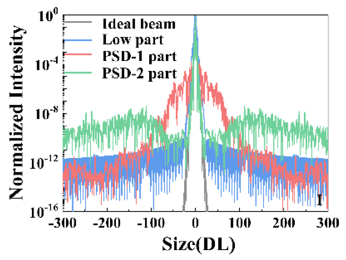
When analyzing the quality and the peak intensity of the focal spot, it is necessary to pay attention to the intensity distribution of the focal sidelobes. The higher the sidelobe intensity, the higher the hole-blocking risk during laser propagation in the amplification chain. The three types wavefronts have similar effects on sidelobe intensity. The influence of different filtered types of wavefront I on the sidelobe intensity is shown in
Figure 9 when the unfiltered original wavefront PV = 2
λ.
From
Figure 9, it can be observed that different spatial-frequency types have different effects on the focal spot. The low-spatial-frequency type mainly affects the intensity distribution near the focal mainlobe. The PSD-1 type mainly affects low-level sidelobes, and PSD-2 mainly affects high-level sidelobes. From the diffraction divergent angle
, the corresponding focal spot size is
, where
λ is the wavelength,
is the spatial period, and
D is the beam aperture. Therefore, the low-spatial-frequency type, PSD-1, and PSD-2 mainly affected the focal spot within approximately 10DL, 10DL-124DL, and larger than 124DL, respectively. In addition, the relative intensity of the focal sidelobes under the low spatial frequency, PSD-1, and PSD-2, are about >10
−4, >10
−9, and >10
−12 when the original wavefront PV = 2
λ, respectively.
The relative intensity of the PSD-2 frequency starts to increase around 50DL, as shown in
Figure 9, and the divergent angle is approximately 170 μrad, which is close to the angle of the aperture radius. To prevent the hole-blocking effect caused by the high energy density of the sidelobe, the intensity of the focal spot at 50DL should not be too high. The relative intensities of the three wavefronts at 50DL are studied, and the variations with the PV value of original wavefront are shown in
Figure 10.
Figure 10 depicts the effect of the PV value on the focal sidelobe intensity with the different spatial-frequency types. In this figure, the separation of the gray and blue curves and the coincidence of the blue and red curves indicate that the relative intensity of 50DL is mainly affected by the low spatial frequency and PSD-1 frequency, while is almost not influenced by the PSD-2 frequency. With the increase in the original wavefront PV, the relative intensity of the sidelobes rises. When PV = 2λ, the relative intensity at 50DL deteriorates to 10
−6–10
−5. If the relative intensity is required to be less than 10
−8, the allowable PV values of wavefronts I, II, and III should not exceed 0.35
λ, 0.37
λ, and 0.37
λ, respectively.


