Thermal Deformation Measurement of Aerospace Honeycomb Panel Based on Fusion of 3D-Digital Image Correlation and Finite Element Method


Abstract
:1. Introduction
2. Methods
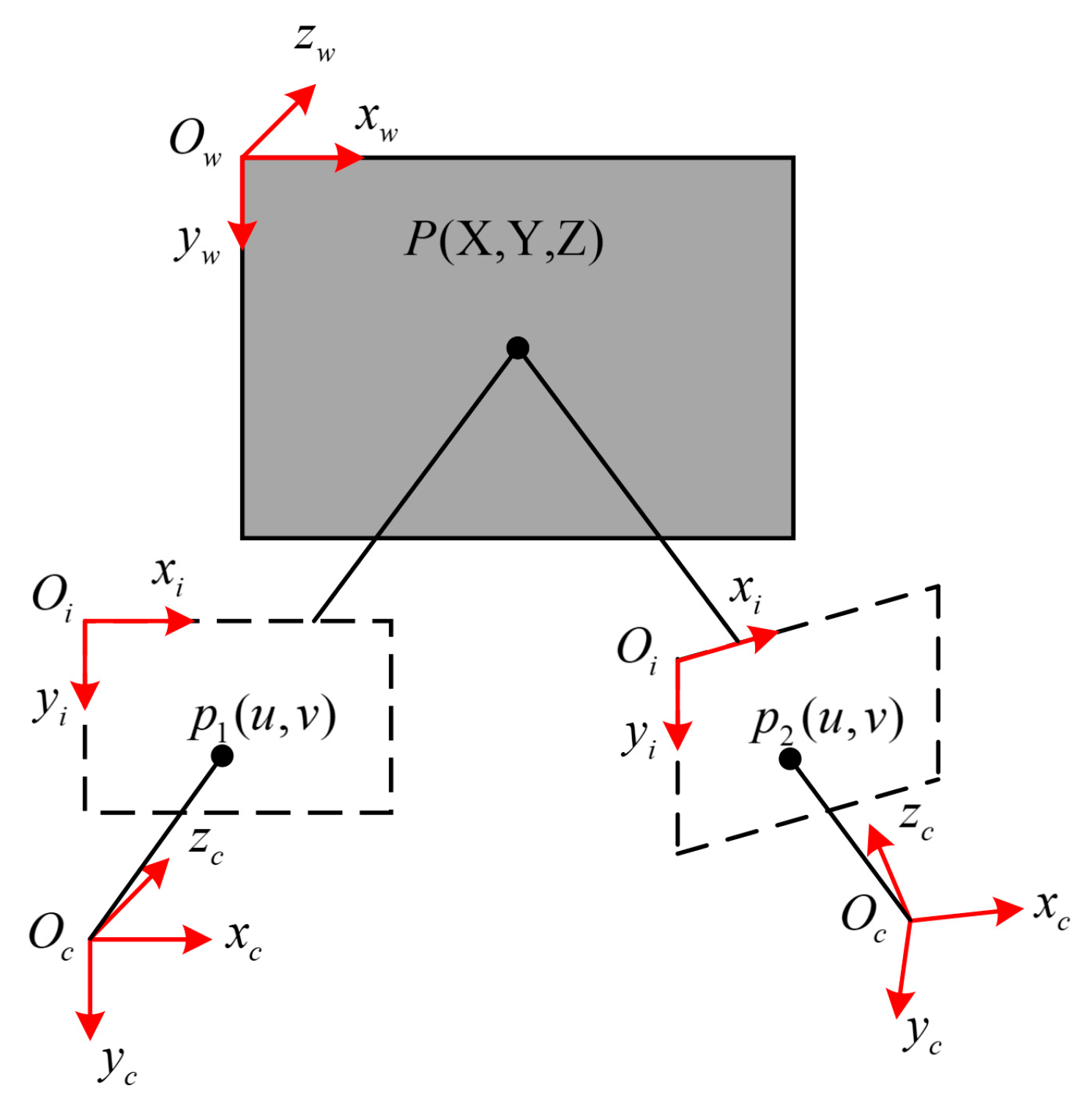
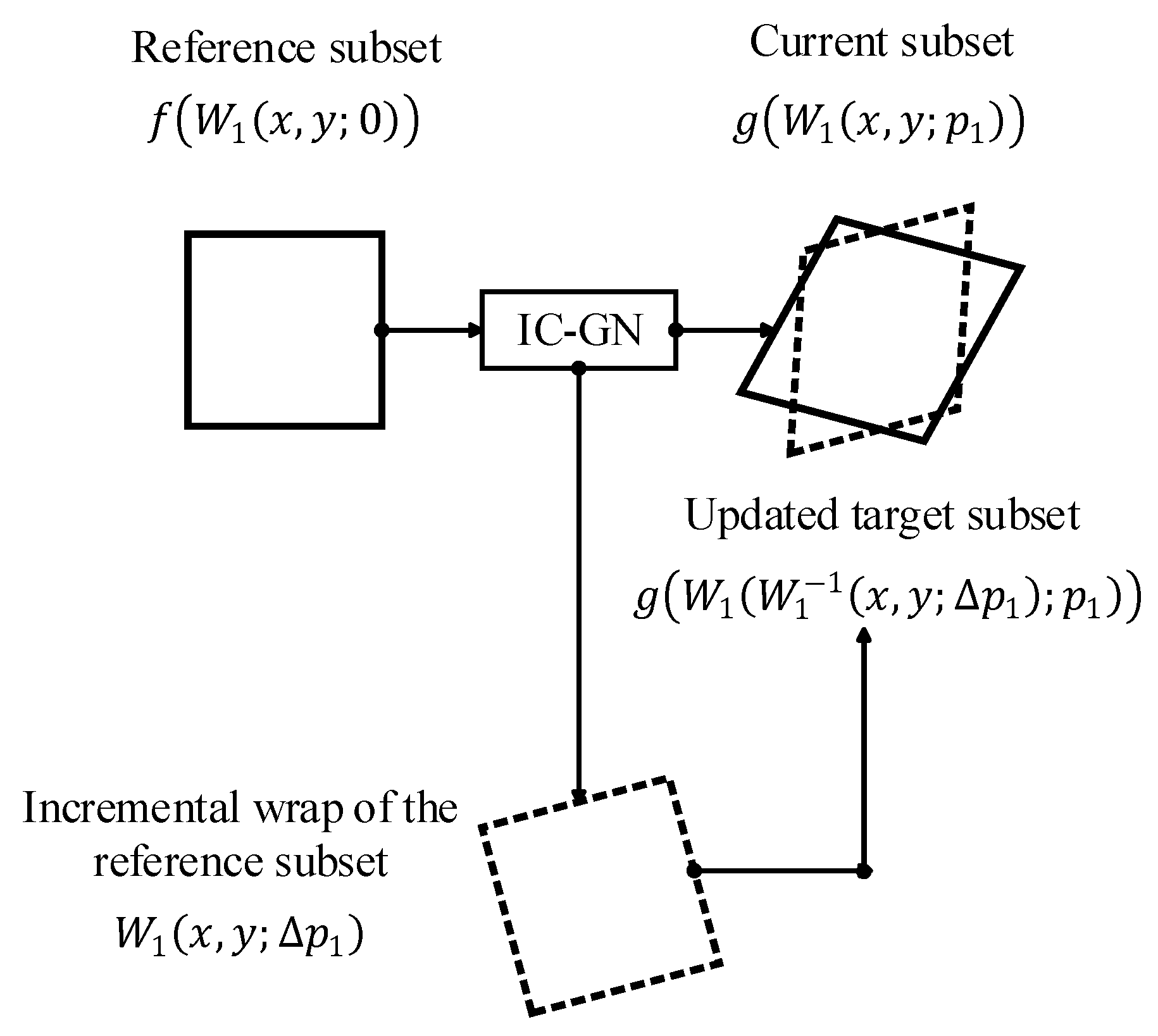
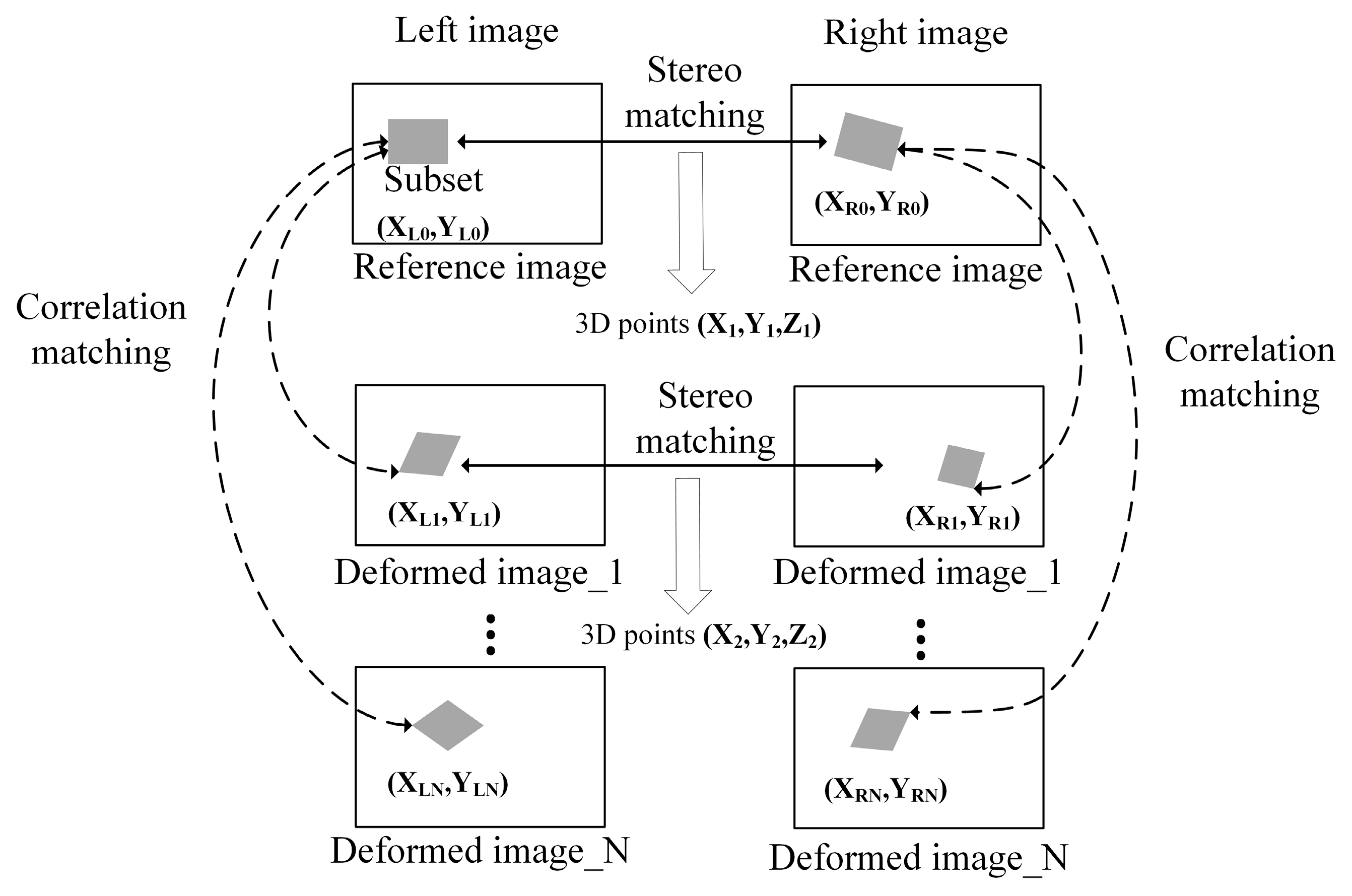
2.1. 3D Digital Image Correlation
- World coordinate system with a point in real space as the origin.
- Camera coordinate system with the camera optical center position as the origin.
- Imaging plane coordinate system taking the intersection point of optical axis and imaging plane as the origin.
- Image coordinate system with the upper left corner of the imaging pixel array plane as the origin.

2.2. Finite Element Model Modification Method
- Geometry parameters: the size and the thickness of the skin.
- Material property parameters: expansion coefficient, Poisson’s ratio.
- Boundary condition parameters: constraint point location.
- Load parameters: temperature load on the structure.
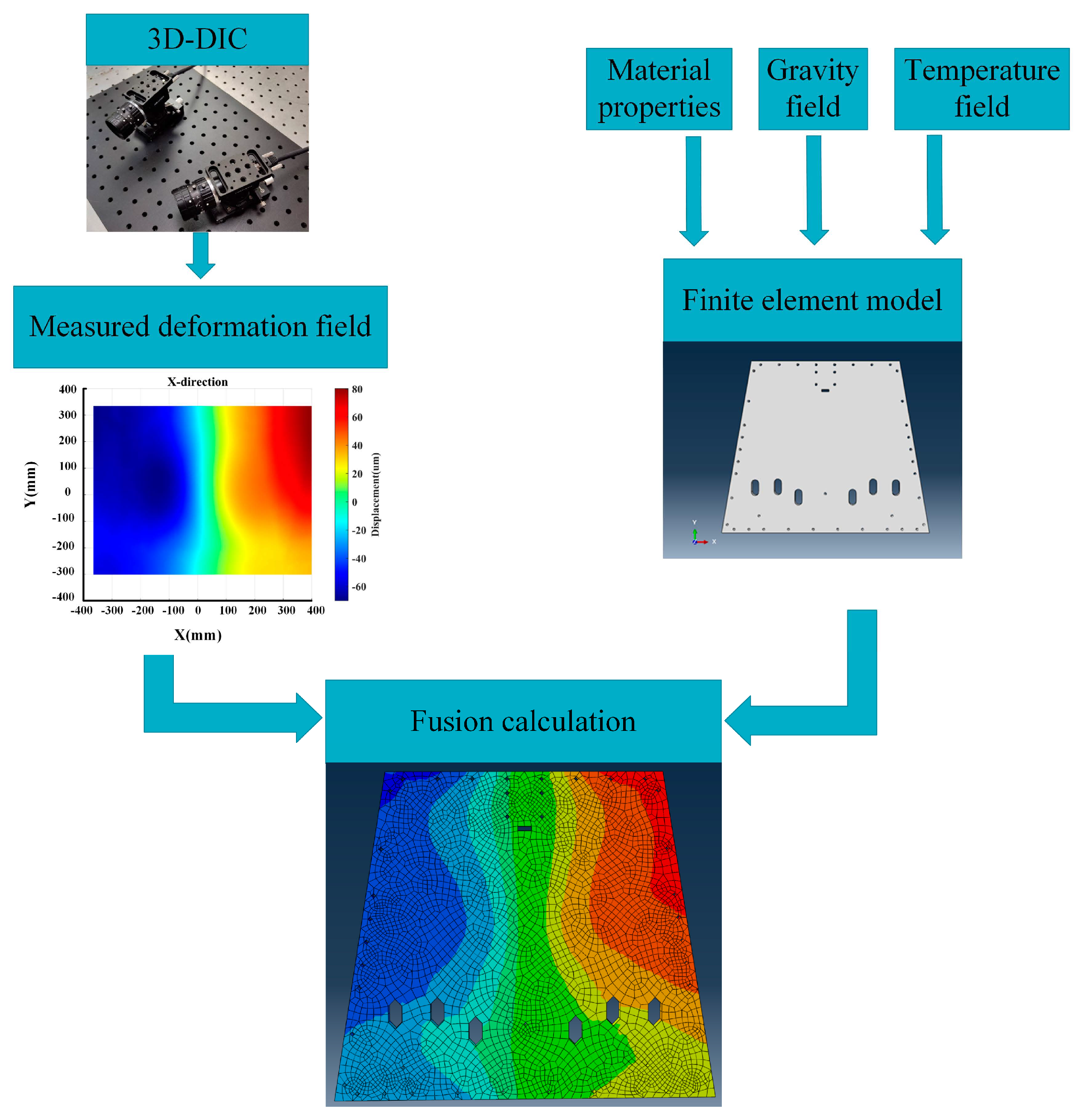
2.3. Design of Fusion Algorithm
2.3.1. Training Data-Set
2.3.2. Network Structure Design
2.3.3. Algorithm
3. Experiments
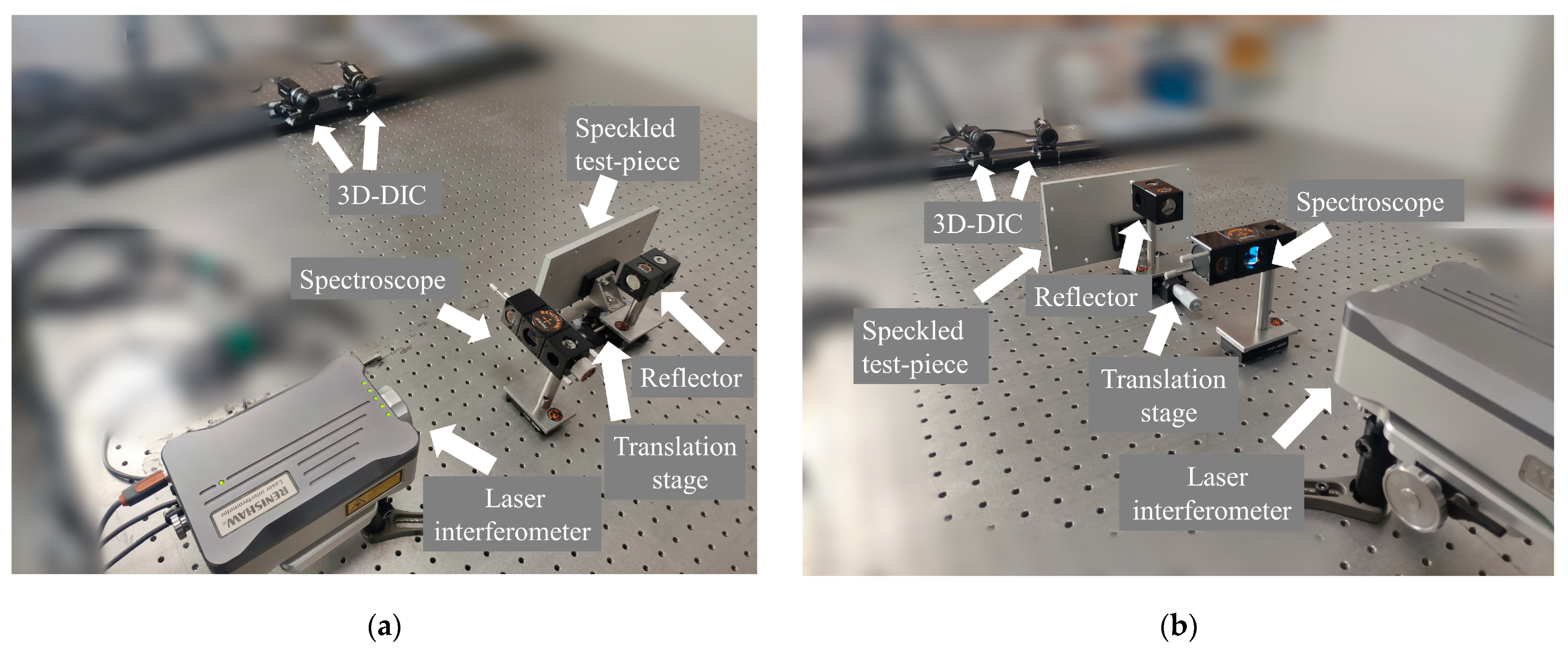
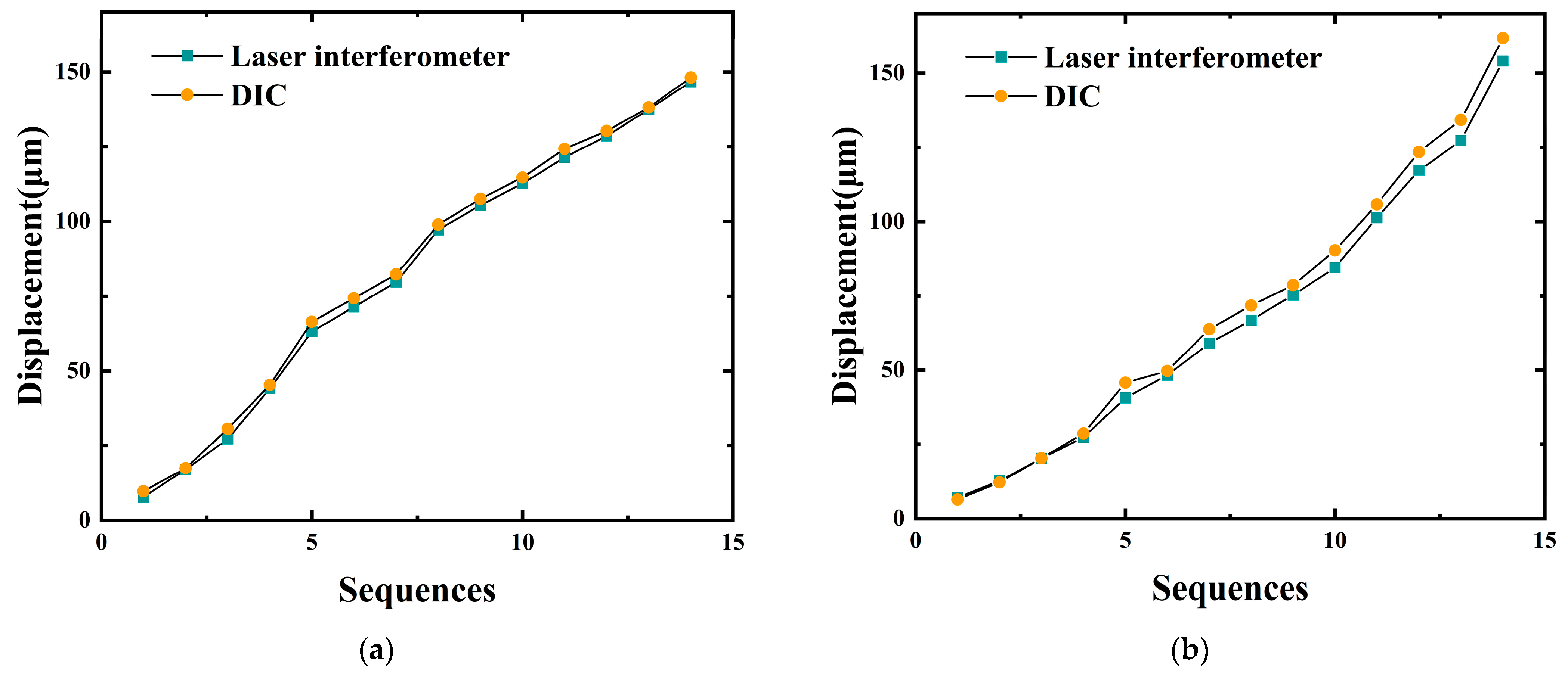
3.1. Construction and Accuracy Verification of 3D-DIC Measurement System
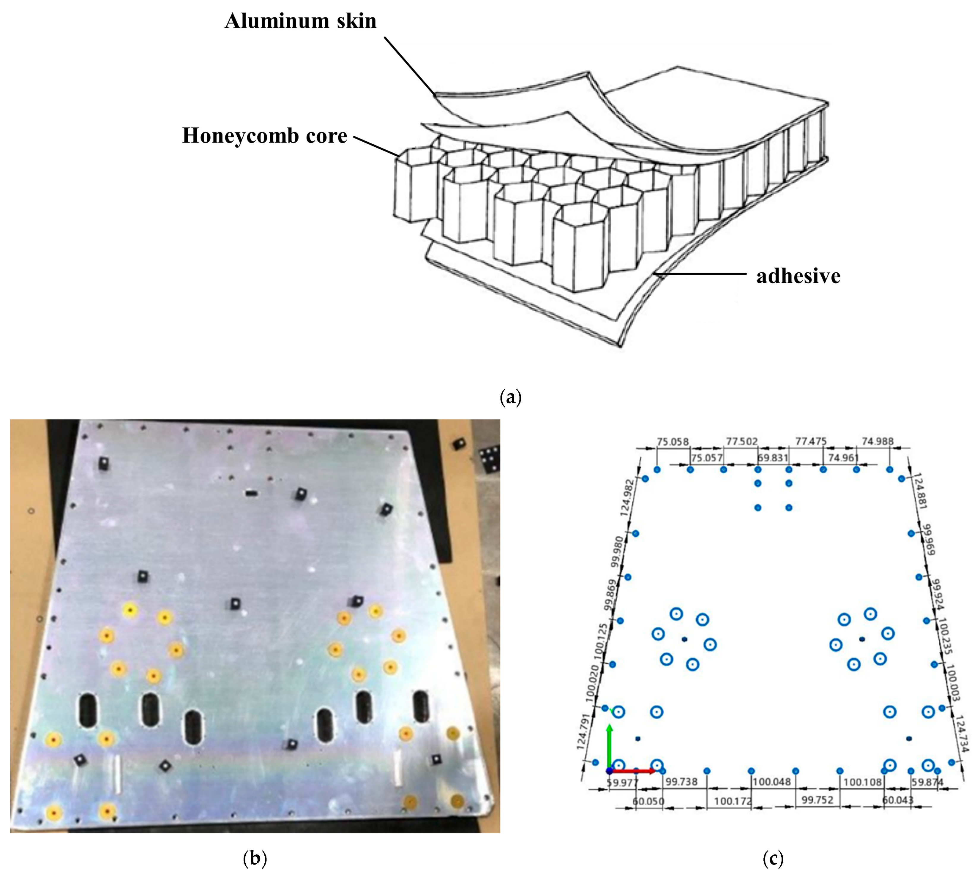
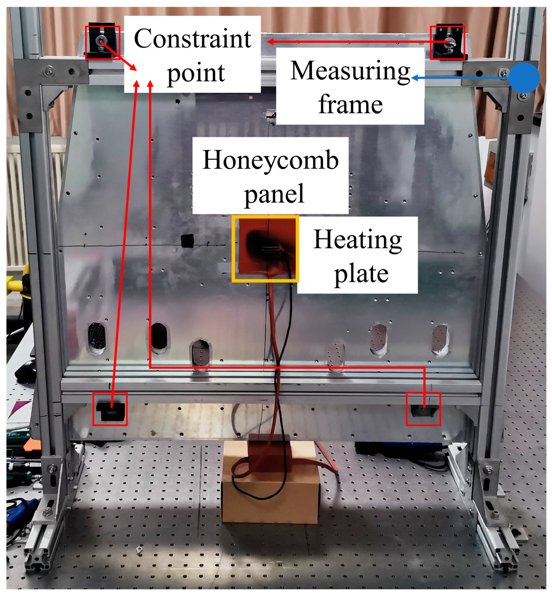
3.2. Measuring System for Honeycomb Panels
3.3. Finite Element Model Modification Experiment
3.3.1. Establishment of Finite Element Model
3.3.2. Establish an Optimization Model
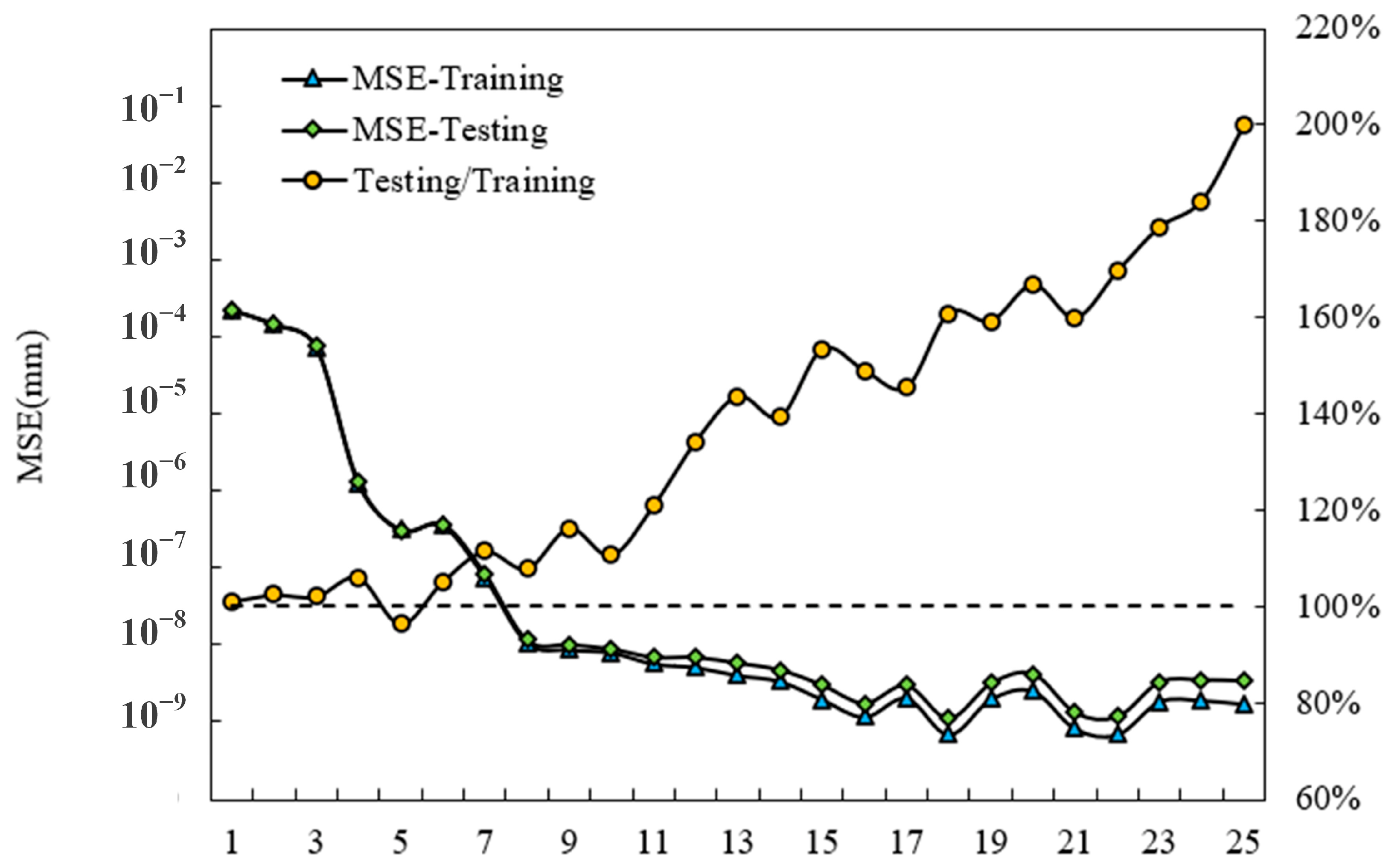
3.3.3. Training BP Neural Network
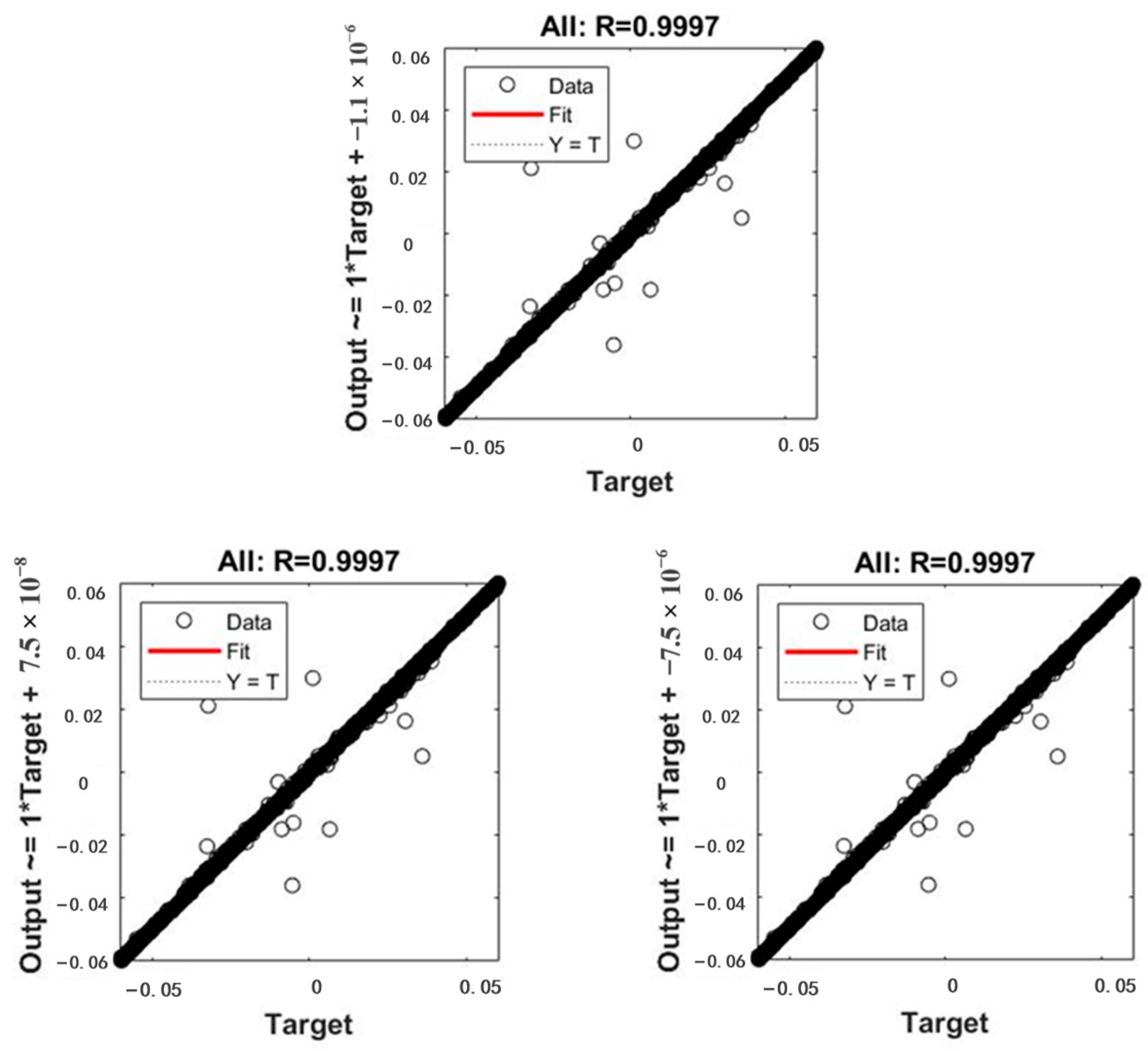
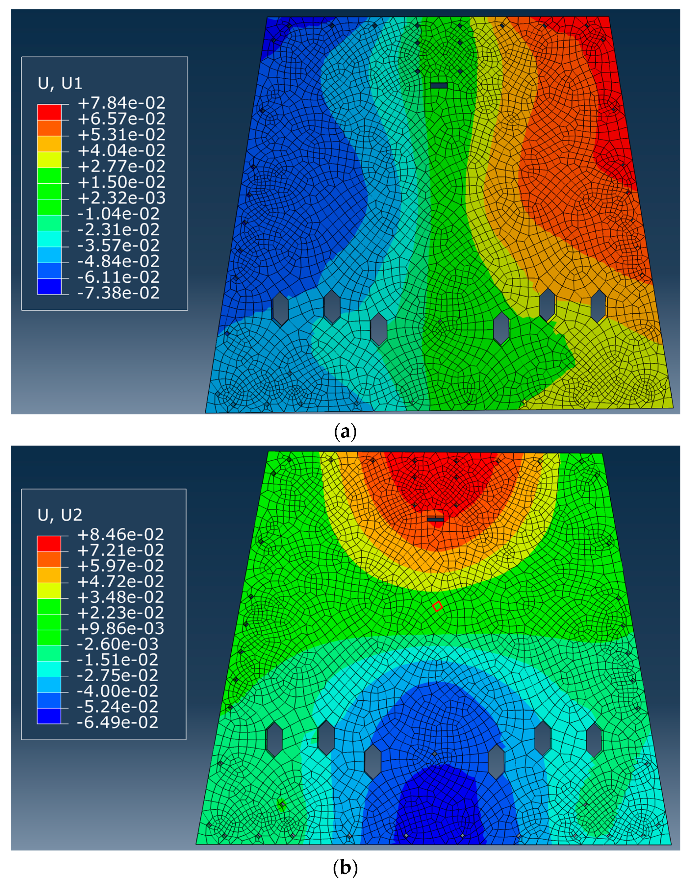
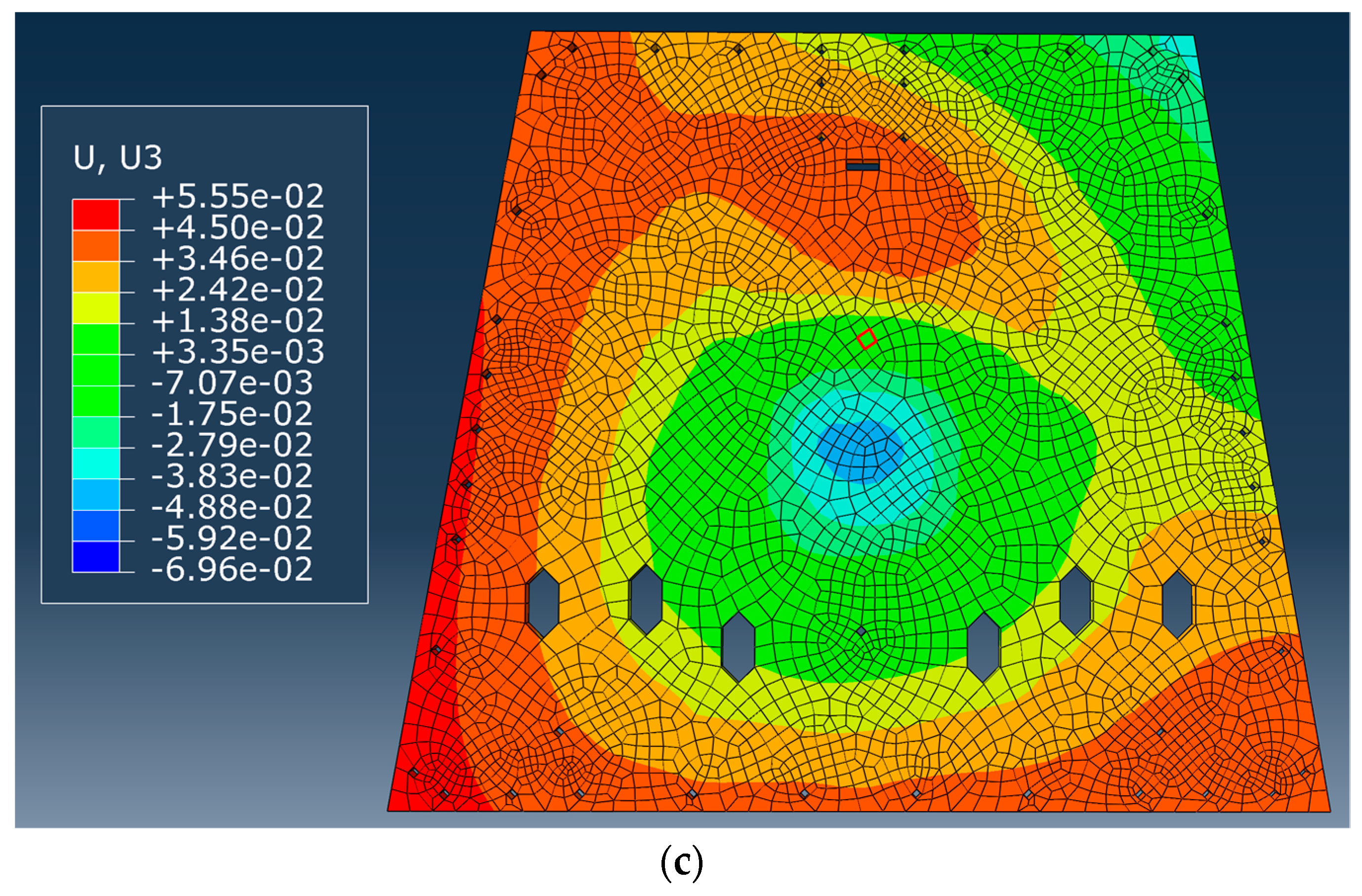
3.4. Accuracy Analysis of Deformation Prediction
4. Conclusions
Author Contributions
Funding
Institutional Review Board Statement
Informed Consent Statement
Data Availability Statement
Conflicts of Interest
References
- Horst, S.; Chrone, J.; Deacon, S.; Le, C.; Maillard, A.; Molthan, A.; Nguyen, A.; Osmanoglu, B.; Oveisgharan, S.; Perrine, M.; et al. NASA’s Surface Deformation and Change Mission Study. In Proceedings of the 2021 IEEE Aerospace Conference, Big Sky, MT, USA, 6–13 March 2021; pp. 1–19. [Google Scholar]
- Corbacho, V.V.; Kuiper, H.; Gill, E. Review on thermal and mechanical challenges in the development of deployable space optics. J. Astron. Telesc. Instrum. Syst. 2020, 6, 010902. [Google Scholar]
- Le, V.T.; San Ha, N.; Goo, N.S. Advanced sandwich structures for thermal protection systems in hypersonic vehicles: A review. Compos. Part B Eng. 2021, 226, 109301. [Google Scholar] [CrossRef]
- Ji, L.; Wang, H. Analysis of On-orbit Thermal Deformation of Flexible SAR Antenna. In Proceedings of the 2021 2nd China International SAR Symposium (CISS), Shanghai, China, 3–5 November 2021; pp. 1–6. [Google Scholar]
- He, Y.; Li, B.; Wang, Z.; Zhang, Y. Thermal Design and Verification of Spherical Scientific Satellite Q-SAT. Int. J. Aerosp. Eng. 2021, 2021, 9961432. [Google Scholar] [CrossRef]
- Shen, Z.; Li, H.; Liu, X.; Hu, G. Thermal-structural dynamic analysis of a satellite antenna with the cable-network and hoop-truss supports. J. Therm. Stress. 2019, 42, 1339–1356. [Google Scholar] [CrossRef]
- Zhang, H.; Zhao, X.; Mei, Q.; Wang, Y.; Song, S.; Yu, F. On-orbit thermal deformation prediction for a high-resolution satellite camera. Appl. Therm. Eng. 2021, 195, 117152. [Google Scholar] [CrossRef]
- Li, J.; Yan, S. Thermally induced vibration of the composite solar array with honeycomb panels in low earth orbit. Appl. Therm. Eng. 2014, 71, 419–432. [Google Scholar] [CrossRef]
- He, M.; Hu, W. A study on composite honeycomb sandwich panel structure. Mater. Des. 2008, 29, 709–713. [Google Scholar] [CrossRef]
- Seo, S.I.; Kim, J.S.; Cho, S.H.; Kim, S.C. Manufacturing and Mechanical Properties of a Honeycomb Sandwich Panel. Mater. Sci. Forum 2008, 580–582, 85–88. [Google Scholar] [CrossRef]
- Wu, M.; Liu, J. Study on Thermal Performance of Single-layer and Multi-layer Stone Aluminum Honeycomb Composite Panels. J. Phys. Conf. Ser. 2019, 1300, 012002. [Google Scholar] [CrossRef]
- Amini, A.; Mohammadimehr, M.; Faraji, A.R. Active control to reduce the vibration amplitude of the solar honeycomb sandwich panels with CNTRC facesheets using piezoelectric patch sensor and actuator. Steel Compos. Struct. 2019, 32, 671–686. [Google Scholar]
- Ibrahim, S.K.; Mccue, R.; O’Dowd, J.A.; Farnan, M.; Karabacak, D.M. Fiber sensing for space applications. In Proceedings of the European Conference on Spacecraft Structures Materials and Environmental Testing (ECSSMET 2018), Noordwijk, The Netherlands, 28 May–1 June 2018. [Google Scholar]
- Aqueeb, A.; Yang, M.; Braaten, B.; Burczek, E.; Roy, S. A Real-Time and Wireless Structural Health Monitoring Scheme for Aerospace Structures Using Fibre Bragg Grating Principle. In Photonics, Plasmonics and Information Optics; CRC Press: Boca Raton, FL, USA, 2021; pp. 241–266. [Google Scholar]
- Wang, X.; Gao, Z.; Yang, S.; Gao, C.; Sun, X.; Wen, X.; Feng, Z.; Wang, S.; Fan, Y. Application of digital shearing speckle pattern interferometry for thermal stress. Measurement 2018, 125, 11–18. [Google Scholar] [CrossRef]
- Shrestha, R.; Kim, W. Non-destructive testing and evaluation of materials using active thermography and enhancement of signal to noise ratio through data fusion. Infrared Phys. Technol. 2018, 94, 78–84. [Google Scholar] [CrossRef]
- Wang, B.; Zhong, S.; Lee, T.-L.; Fancey, K.S.; Mi, J. Non-destructive testing and evaluation of composite materials/structures: A state-of-the-art review. Adv. Mech. Eng. 2020, 12, 1687814020913761. [Google Scholar] [CrossRef] [Green Version]
- Kudela, P.; Wandowski, T.; Malinowski, P.; Ostachowicz, W. Application of scanning laser Doppler vibrometry for delamination detection in composite structures. Opt. Lasers Eng. 2016, 99, 46–57. [Google Scholar] [CrossRef]
- Liu, G.; Jianhua, R.; Luo, W. Research on Thermal Deformation Analysis and Test Verification Method for Spacecraft High-stability Structure. Spacecr. Eng. 2014, 23, 64–70. [Google Scholar]
- Jiang, S.; Yang, L.; Xu, J.; Yu, J. Deformation measurement for satellite antenna by close-range photogrammetry. In Proceedings of the SPIE—The International Society for Optical Engineering, San Diego, CA, USA, 25–29 August 2013; p. 8896. [Google Scholar]
- Blanchard, A.; Kosmatov, N.; Loulergue, F. A Lesson on Verification of IoT Software with Frama-C. In Proceedings of the 2018 International Conference on High Performance Computing & Simulation, Orléans, France, 16–20 July 2018. [Google Scholar]
- De Angelis, G.; Meo, M.; Almond, D.P. A new technique to detect defect size and depth in composite structures using digital shearography and unconstrained optimization. NDT E Int. Indep. Nondestruct. Test. Eval. 2012, 45, 91–96. [Google Scholar] [CrossRef]
- Yumuş, C.; Atici, G.; Duman, C. Thermomechanical Design and Analysis of Waveguides on Communication Satellite Payloads. In Proceedings of the 2019 9th International Conference on Recent Advances in Space Technologies (RAST), Istanbul, Turkey, 11–14 June 2019; pp. 363–367. [Google Scholar]
- Qian, Z.; Luo, W.; Yin, Y.; Zhang, L.; Bai, G.; Cai, Z.; Fu, W.; Lu, Q.; Zhang, X.; Zhao, C. Dimensional stability design and verification of GF-7 satellite structure. Chin. Space Sci. Technol. 2020, 40, 10. [Google Scholar]
- Mao, J.; Zhang, W.H. Engineering Applications of Satellite Structural Optimization Utilizing ANSYS/CATIA. Appl. Mech. Mater. 2012, 110–116, 1567–1575. [Google Scholar] [CrossRef]
- Güvenç, C.; Topcu, B.; Tola, C. Mechanical design and finite element analysis of a 3 unit cubesat structure. Mach. Technol. Mater. 2018, 12, 193–196. [Google Scholar]
- Halloin, H.; Jeannin, O.; Argence, B.; Bourrier, V.; De Vismes, E.; Prat, P. Lisa on table: An optical simulator for lisa. In Proceedings of the International Conference on Space Optics 2010, Rhodes Island, Greece, 4–8 October 2010; Society of Photo-Optical Instrumentation Engineers (SPIE) Conference Series; SPIE: Washington, DC, USA, 2017. [Google Scholar] [CrossRef] [Green Version]
- Kovács, R.; Józsa, V. Thermal analysis of the SMOG-1 PocketQube satellite. Appl. Therm. Eng. 2018, 139, 506–513. [Google Scholar] [CrossRef]
- Ca Lvi, A. An Overview of the E.C.S.S. In Handbook for Spacecraft Loads Analysis, Proceedings of the III ECCOMAS Thematic Conference on Computational Methods in Structural Dynamics and Earthquake Engineering, Corfu, Greece, 12–14 June 2013; ECCOMAS: Barcelona, Spain, 2014; Available online: https://www.eccomasproceedia.org/conferences/thematic-conferences/compdyn-2013 (accessed on 15 November 2022).
- Owens, A.T.; Tippur, H.V. Measurement of mixed-mode fracture characteristics of an epoxy-based adhesive using a hybrid digital image correlation (DIC) and finite elements (FE) approach. Opt. Lasers Eng. 2021, 140, 106544. [Google Scholar] [CrossRef]
- Balcaen, R.; Wittevrongel, L.; Reu, P.L.; Lava, P.; Debruyne, D. Stereo-DIC calibration and speckle image generator based on FE formulations. Exp. Mech. 2017, 57, 703–718. [Google Scholar] [CrossRef]
- Siddiqui, M.Z. 2D-DIC for the quantitative validation of FE simulations and non-destructive inspection of aft end debonds in solid propellant grains. Aerosp. Sci. Technol. 2014, 39, 128–136. [Google Scholar] [CrossRef]
- Babaeeian, M.; Mohammadimehr, M. Investigation of the time elapsed effect on residual stress measurement in a composite plate by DIC method. Opt. Lasers Eng. 2020, 128, 106002. [Google Scholar] [CrossRef]
- Ross-Pinnock, D.; Yang, B.; Maropoulos, P.G. Integration of Thermal and Dimensional Measurement—A Hybrid Computational and Physical Measurement Method. In Proceedings of the 38th International MATADOR Conference, Huwei, Taiwan, 28–31 March 2015; Springer: Cham, Switzerland, 2022; pp. 627–639. [Google Scholar]
- De Chiffre, L.; González-Madruga, D.; Sonne, M.R.; Costa, G.D.; Hattel, J.H.; Hansen, H.N. Dynamic length metrology (DLM) for accurate dimensional measurements in a production environment by continuous determination and compensation of thermal expansion effects in turning steel. Meas. Sci. Technol. 2021, 32, 094007. [Google Scholar] [CrossRef]
- Schulte, M.J.; Omar, J.; Swartzlander, E.E. Optimal initial approximations for the Newton-Raphson division algorithm. Computing 2015, 53, 233–242. [Google Scholar] [CrossRef]
- Bai, R.; Jiang, H.; Lei, Z.; Li, W. A novel 2nd-order shape function based digital image correlation method for large deformation measurements. Opt. Lasers Eng. 2017, 90, 48–58. [Google Scholar] [CrossRef]
- Aborehab, A.; Kassem, M.; Nemnem, A.; Kamel, M. Miscellaneous modeling approaches and testing of a satellite honeycomb sandwich plate. J. Appl. Comput. Mech. 2019, 6, 1084–1097. [Google Scholar]


| System accuracy | ±0.5 ppm (±0.5 μm/m) |
| Laser frequency stabilization accuracy | ±0.05 ppm (±0.05 μm/m) |
| Resolution | 1 nm |
| Measuring range | 80 m |
| Maximum measuring speed | 4 m/s |
| Parameter | Value | ||
|---|---|---|---|
| Aluminum skin | Modulus of elasticity | 68,000 MPa | |
| Poisson’s ratio | 0.36 | ||
| Coefficient of expansion | 2.32 × 10⁻⁵/°C | ||
| Honeycomb core | Modulus of elasticity | E1 | 0.0339 MPa |
| E2 | 0.0339 MPa | ||
| E3 | 800 MPa | ||
| Poisson’s ratio | Nu12 | 0.33 | |
| Nu13 | 0 | ||
| Nu23 | 0 | ||
| Shear modulus | G12 | 0.0065 MPa | |
| G13 | 45.58 MPa | ||
| G23 | 68.37 MPa | ||
| Coefficient of expansion | 2.3 × 10⁻⁵/°C | ||
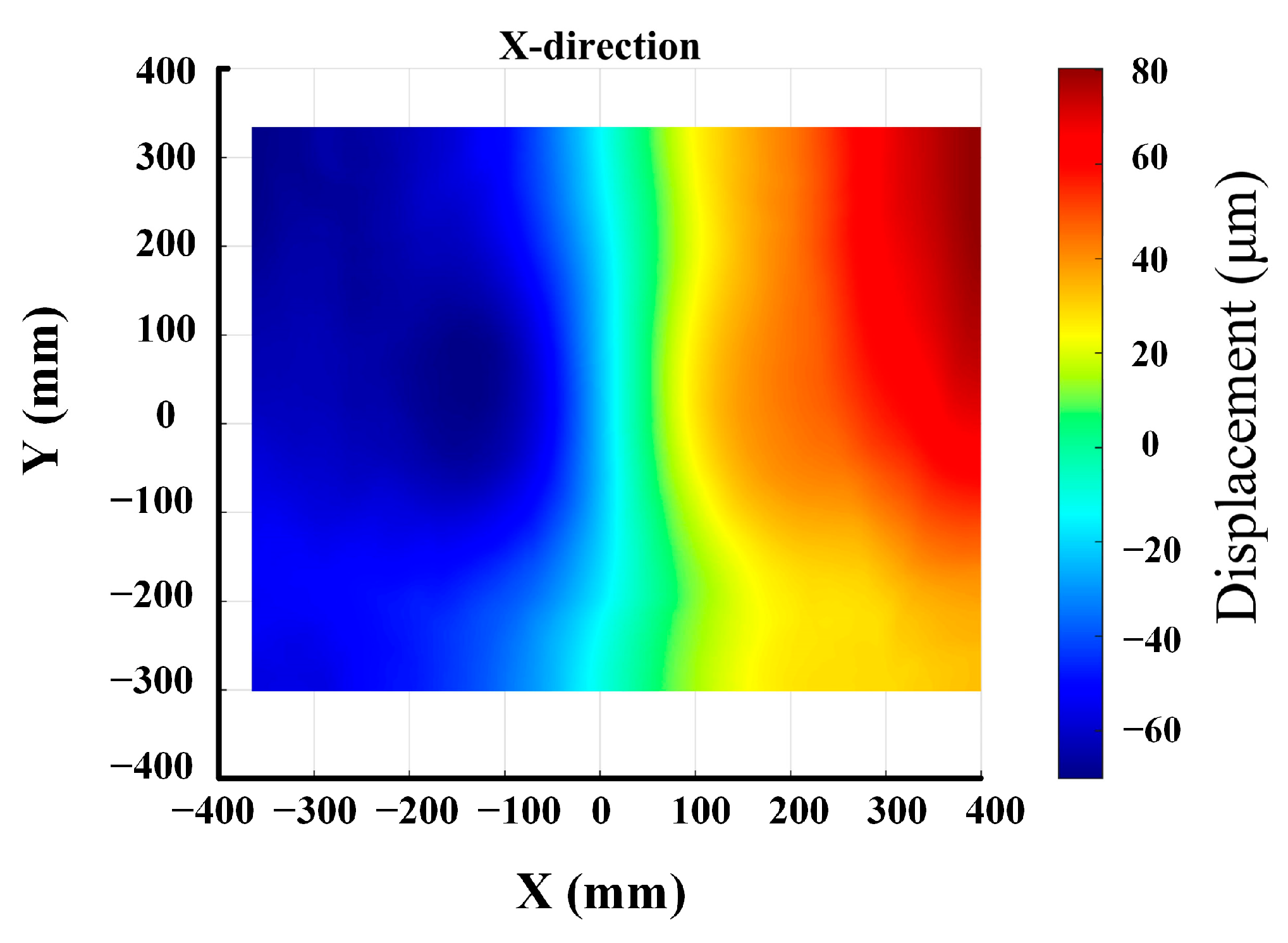
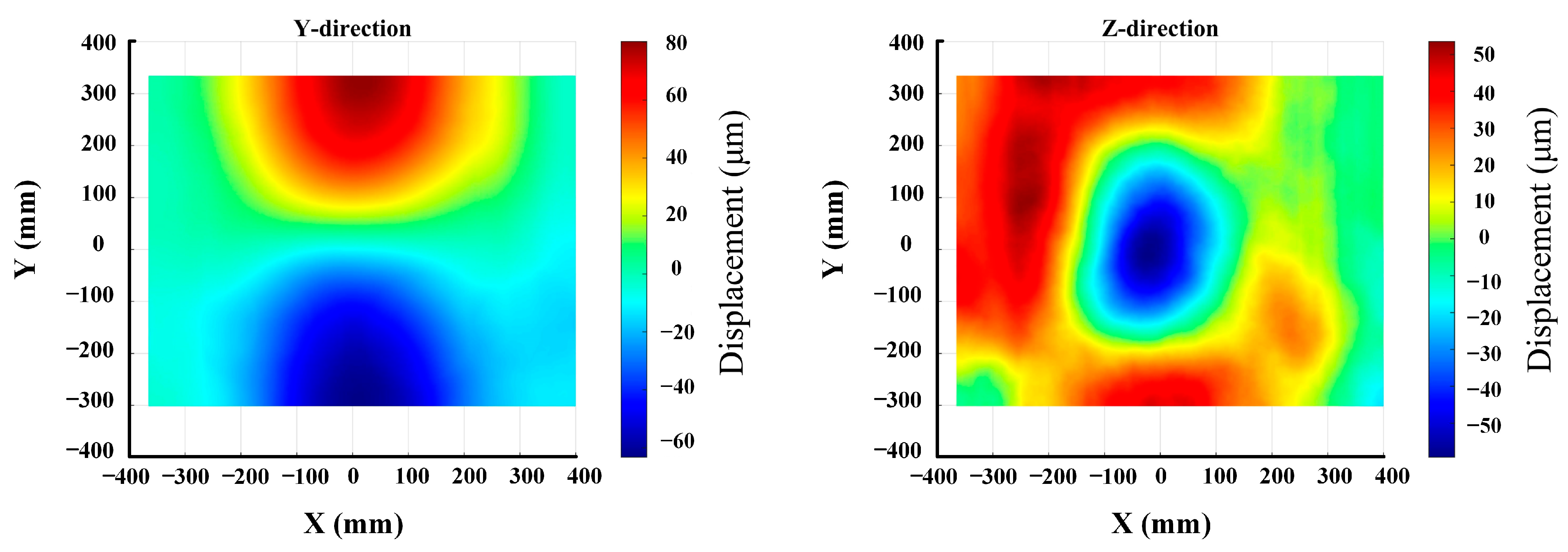
| Displacement | X/μm | Y/μm | Z/μm |
|---|---|---|---|
| Fixed point 1 | −55.26 | 14.36 | 37.47 |
| Fixed point 2 | 62.59 | 30.01 | −12.50 |
| Fixed point 3 | −40.77 | −2.88 | 18.73 |
| Fixed point 4 | 19.27 | −10.06 | 21.36 |
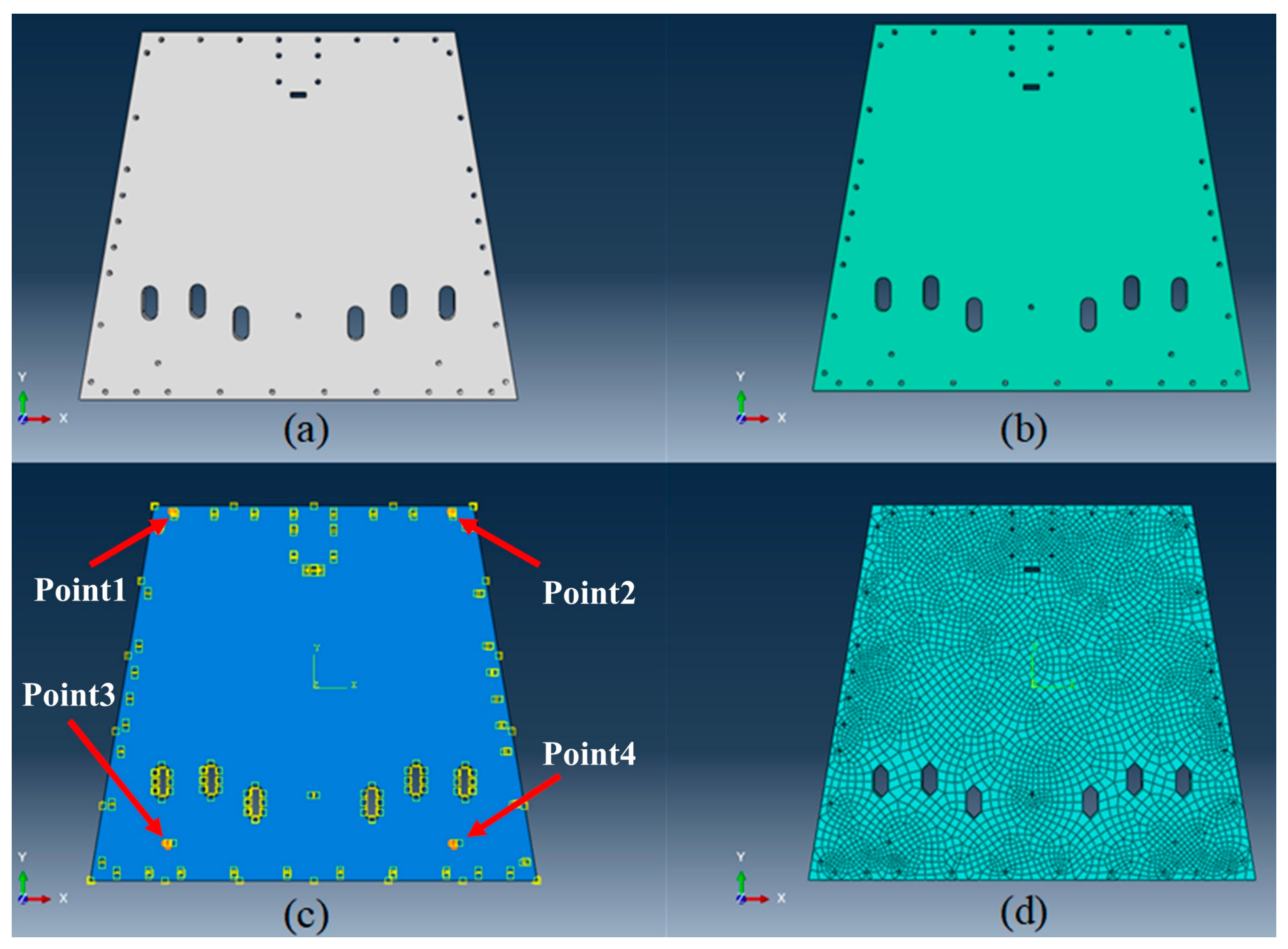
| ID | X/mm | Y/mm |
|---|---|---|
| Point 1 | −278.434 | 280.106 |
| Point 2 | 3.143 | 280.160 |
| Point 3 | 277.812 | 281.114 |
| Point 4 | −298.643 | 84.553 |
| Point 5 | −1.014 | 84.093 |
| Point 6 | 297.361 | 83.892 |
| Point 7 | −323.300 | −104.062 |
| Point 8 | −2.406 | −104.195 |
| Point 9 | 325.165 | −103.593 |
| Point 10 | −344.058 | −286.581 |
| Point 11 | 1.602 | −284.850 |
| Point 12 | 347.026 | −285.388 |
| Parameter | Sensitivity | ||
|---|---|---|---|
| Aluminum skin | Modulus of elasticity | 6.00 × 10⁻⁵ | |
| Poisson’s ratio | 7.78 × 10⁻⁴ | ||
| Coefficient of expansion | 4.5 × 10⁻³ | ||
| Honeycomb core | Modulus of elasticity | E1 | 1.65 × 10⁻⁸ |
| E2 | 2.32 × 10⁻⁸ | ||
| E3 | 2.88 × 10⁻⁶ | ||
| Poisson’s ratio | Nu12 | 1.04 × 10⁻⁸ | |
| Nu13 | - | ||
| Nu23 | - | ||
| Shear modulus | G12 | 8.01 × 10⁻⁹ | |
| G13 | 5.41 × 10⁻⁵ | ||
| G23 | 5.17 × 10⁻⁵ | ||
| Coefficient of expansion | 2.29 × 10⁻⁴ | ||
| Material property parameters | Skin expansion coefficient, Poisson’s ratio, honeycomb core expansion coefficient |
| Boundary condition parameters | Displacement parameters of fixed points 1–4 |
| Parameter | Range of Disturbance |
|---|---|
| Coefficient of skin expansion | ±0.02 × 10⁻⁵/°C |
| Poisson’s ratio of skin expansion | |
| The expansion coefficient of the honeycomb core | ±0.02 × 10⁻⁵/°C |
| Displacement of fixed points | μm |
| Number of Neurons in the Hidden Layer | The Hidden Layer Response Function | Output Layer Response Function | Optimization Function | Gradient Threshold | Error Function |
|---|---|---|---|---|---|
| 10 | tansig | purelin | BR | 1 × 10⁻⁷ | MSE |
| Parameter | Value | |
|---|---|---|
| The expansion coefficient of skin Poisson’s ratio of skin The expansion coefficient of the honeycomb core | 2.33 × 10⁻⁵/°C | |
| 0.362 | ||
| 2.30 × 10⁻⁵/°C | ||
| Displacement parameters of fixed point 1 | X-direction | −62.03 μm |
| Y-direction | 1.60 μm | |
| Z-direction | 37.22 μm | |
| Displacement parameters of fixed point 2 | X-direction | 70.15 μm |
| Y-direction | 11.36 μm | |
| Z-direction | −27.54 μm | |
| Displacement parameters of fixed point 3 | X-direction | −39.98 μm |
| Y-direction | −0.61 μm | |
| Z-direction | 35.66 μm | |
| Displacement parameters of fixed point 4 | X-direction | 28.70 μm |
| Y-direction | −7.73 μm | |
| Z-direction | 36.85 μm | |
| Parameter | Value | |
|---|---|---|
| The expansion coefficient of skin Poisson’s ratio of skin The expansion coefficient of the honeycomb core | 2.33 × 10⁻⁵/°C | |
| 0.362 | ||
| 2.30 × 10⁻⁵/°C | ||
| Displacement parameters of fixed point 1 | X-direction | −34.59 μm |
| Y-direction | 1.36 μm | |
| Z-direction | 21.45 μm | |
| Displacement parameters of fixed point 2 | X-direction | 36.32 μm |
| Y-direction | 7.91 μm | |
| Z-direction | −16.52 μm | |
| Displacement parameters of fixed point 3 | X-direction | −20.77 μm |
| Y-direction | −0.34 μm | |
| Z-direction | 14.76 μm | |
| Displacement parameters of fixed point 4 | X-direction | 13.79 μm |
| Y-direction | −3.36 μm | |
| Z-direction | 25.45 μm | |
Disclaimer/Publisher’s Note: The statements, opinions and data contained in all publications are solely those of the individual author(s) and contributor(s) and not of MDPI and/or the editor(s). MDPI and/or the editor(s) disclaim responsibility for any injury to people or property resulting from any ideas, methods, instructions or products referred to in the content. |
© 2023 by the authors. Licensee MDPI, Basel, Switzerland. This article is an open access article distributed under the terms and conditions of the Creative Commons Attribution (CC BY) license (https://creativecommons.org/licenses/by/4.0/).
Share and Cite
Yang, L.; Fan, Z.; Wang, K.; Sun, H.; Hu, S.; Zhu, J. Thermal Deformation Measurement of Aerospace Honeycomb Panel Based on Fusion of 3D-Digital Image Correlation and Finite Element Method. Photonics 2023, 10, 217. https://doi.org/10.3390/photonics10020217
Yang L, Fan Z, Wang K, Sun H, Hu S, Zhu J. Thermal Deformation Measurement of Aerospace Honeycomb Panel Based on Fusion of 3D-Digital Image Correlation and Finite Element Method. Photonics. 2023; 10(2):217. https://doi.org/10.3390/photonics10020217
Chicago/Turabian StyleYang, Linghui, Zezhi Fan, Ke Wang, Hui Sun, Shuotao Hu, and Jigui Zhu. 2023. "Thermal Deformation Measurement of Aerospace Honeycomb Panel Based on Fusion of 3D-Digital Image Correlation and Finite Element Method" Photonics 10, no. 2: 217. https://doi.org/10.3390/photonics10020217