1. Introduction
Precise and fast estimation of quality of transmission (QoT) for a lightpath prior to its deployment becomes capital for network optimization [
1]. Traditional physical layer model (PLM)-based QoT estimation utilizes optical signal transmission theories to predict the lightpaths’ QoT values, which mainly includes two approaches: (1) sophisticated analytical models, such as the split-step Fourier method [
2]; (2) approximated analytical models, such as the Gaussian Noise (GN) model [
3]. The former approach analyzes various physical layer impairments and provides high estimation accuracy, but it requires high computational resources. Thus, sophisticated analytical models are unable to estimate the lightpaths’ QoT values online and are not scalable to large-scale networks and dynamic network scenarios [
2], and the latter approach, of which the widely used GN model simplifies the nonlinear interference (NLI) to additive Gaussian noise, provides quick QoT estimation for lightpaths, but it requires an extra design margin to ensure the reliability of the lightpaths’ transmission in the worst-case, thus leading to underutilization of network resources [
3]. The PLM-based QoT estimation cannot ensure high accuracy and low computational complexity simultaneously.
Machine learning (ML) has powerful data mining and fast prediction abilities, it has been widely used for QoT estimation. Most of the existing studies focus on the QoT estimation for a signal lightpath [
4,
5,
6,
7,
8,
9,
10,
11,
12,
13,
14,
15,
16,
17,
18,
19,
20], and all of these achieve high accuracy. For example, in [
4], three ML-based classifiers, which include random forest (RF), support vector machine (SVM), and K-nearest neighbor (KNN), are proposed to predict the QoT of lightpaths. The simulation results show that these classifiers achieve high accuracy and the SVM-based classifier achieves the best performance with a classification accuracy of 99.15%. In [
9], a neural network (NN)-based QoT regressor is proposed, and the experimental results show that the regressor achieves a 90% optical signal-to-noise (OSNR) prediction of a 0.25 dB root-mean-squared-error (RMSE) on a mesh network. In [
15], a meta-learning assisted training framework for an ML-based PLM is proposed, and the framework can improve the model robustness to uncertainties of the parameters and enable the model to converge with few data samples. In [
20], it is explored how ML can be used to achieve lightpath QoT estimation and forecast tasks, and the data processing strategies are discussed with the aim to determine the input features of the QoT classifiers and predictors.
However, due to the nonlinear effect of fibers, the newly deployed lightpaths (new-LPs) degrade the QoT of previously deployed lightpaths (pre-LPs). The single-channel (lightpath) QoT estimation only provides the QoT information of the new-LPs, which leads to the decrease in QoT estimation accuracy of the pre-LPs. Thus, it is necessary to estimate the QoT of new-LPs and pre-LPs simultaneously, i.e., multi-channel QoT estimation. In [
21], a deep grapy convolutional neural network (DGCNN)-based QoT classifier is proposed, of which the aim is to accurately classify any unseen lightpath state. In [
22], a novel deep convolutional neural network (DCNN)-based QoT classifier is proposed for network-wide QoT estimation. The above works achieve high accuracy of multi-channel QoT classification. Nevertheless, the QoT classifier cannot provide detailed QoT values of lightpaths; thus, it cannot be directly applied to network planning, such as modulation format assignment. Reference [
23] proposes an ANN-based multi-channel QoT estimator (ANN-QoT-E) over a 563.4 km field-trial testbed, and the mean absolute error (MAE) is about 0.05 dB for the testing data. However, in optical networks, there exist three NLIs, i.e., self-channel interference (SCI), cross-channel interference (XCI), and multi-channel interference (MCI). When the interfering channel with a higher power is closer to the spectrum of the channel under test (CUT), stronger NLI is introduced on the CUT [
3]. Thus, the effects of the interfering channels on the CUTs’ QoT are different. The ANN-QoT-E proposed in [
23] neglects the different effects of the interfering channels in its input layer, which affects its accuracy. Therefore, how to assign different weights to interfering channels for the QoT estimation of CUTs to enhance the accuracy becomes a crucial problem.
In this paper, we extend our previous work in [
24], which applies self-attention mechanisms to improve the accuracy of the ANN-QoT-E. The comparison of this work with the previous works is shown in
Table 1, and the main contributions of this paper are summarized as follows:
- (1)
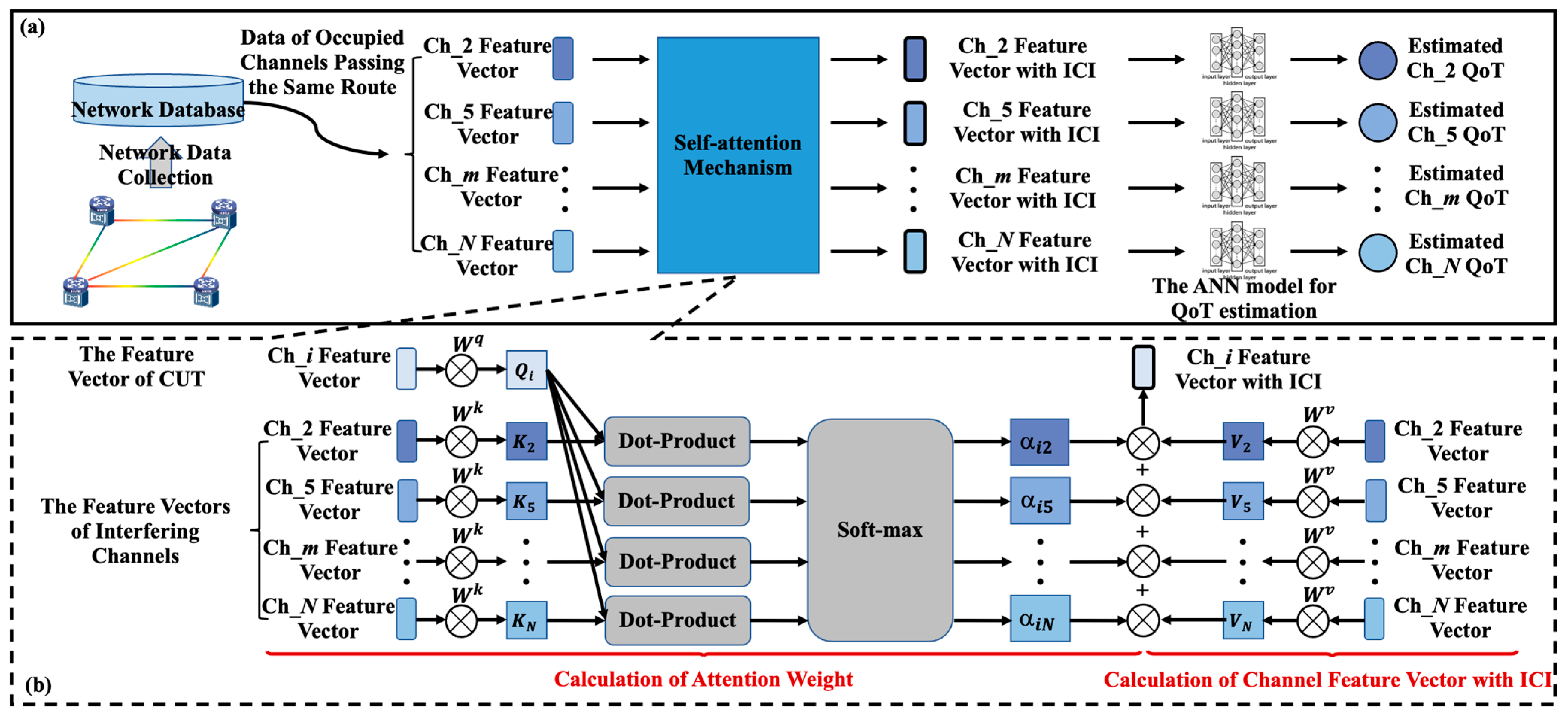
We propose a self-attention mechanism-based multi-channel QoT estimator (SA-QoT-E) to improve the estimation accuracy of the ANN-QoT-E, where the input features are designed as a sequence of channel feature vectors, and the self-mechanism dynamically assigns weights to the interfering channels for the QoT estimation of the CUTs.
- (2)
We use a hyperparameter search method to optimize the SA-QoT-E, which selects optimal hyperparameters for the SA-QoT-E to improve its estimation accuracy.
- (3)
We show the performance of the SA-QoT-E via extensive simulations. The simulation results show that the SA-QoT-E achieves a higher estimation accuracy than the ANN-QoT-E proposed in [
23], and it is verified that the assignment of attention weights to the interfering channels conforms to the optical transmission theory. Compared with the ANN-QoT-E, the SA-QoT-E is more scalable, and it can be directly applied to network wavelength expansion scenarios without retraining. By analyzing the computational complexity of the SA-QoT-E and the ANN-QoT-E, it is concluded that the SA-QoT-E has higher computational complexity. However, the training phase of QoT estimators is offline and the computational complexity of the SA-QoT-E is acceptable; thus, the SA-QoT-E still has more advantages than the ANN-QoT-E in practical network applications.
The remainder of this paper is organized as follows. In
Section 2, we describe the principle of the self-attention mechanism-based multi-channel QoT estimation scheme. The dataset generation and simulation setup are shown in
Section 3. In
Section 4, we discuss the simulation results in terms of convergence, estimation accuracy, scalability, and computational complexity. Finally, we make a conclusion in
Section 5.
3. Data Generation and Simulation Setup
In the SA-QoT-E, the input is the feature vectors of all occupied channels passing the same route, and the output is the generalized signal-to-noise ratio (GSNR) values of these channels. The GSNR can be calculated as follows:
where
is the launch power of the lightpath,
is the amplified spontaneous emission (ASE) noise power introduced by erbium-doped fiber amplifiers (EDFAs), and
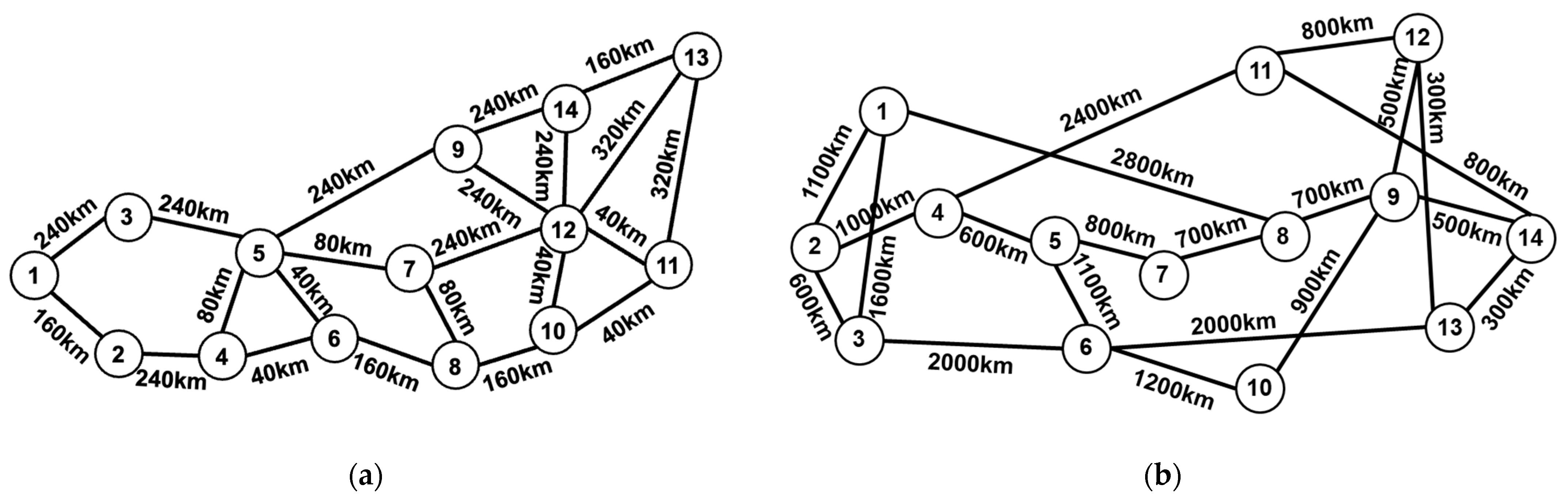
is the NLI power due to the nonlinear effect of fibers. The Japan network (Jnet) and National Science Foundation network (NSFnet) are considered in our simulations, which are shown in
Figure 2a,b, respectively. The transponders of the two networks are set to work on the C++ band of which the center frequency is 193.35 THz with a spectral load with 80 wavelengths (i.e., channels) on the 50 GHz spectral grid. The symbol rate of the transponders is 32 GBaud, and the launch power of each channel is uniformly selected in the range of [−3~0] dBm with 0.1 dBm granularity. We assume the fibers in the two networks are ITU-T G.652 standard single-mode fibers (SSMF), of which attenuation, dispersion, and non-linearity coefficients are 0.2 dB/km, 16.7 ps/nm/km, and 1.3/W/km, respectively; the span length of the fibers is 40 km in the Jnet and 100 km in the NSFnet. The EDFas in the two networks are set to completely compensate for fiber span losses, and the noise figure is 8 dB in the Jnet and 6.5 dB in the NSFnet. The network datasets of the two networks are generated synthetically by the open-source Gaussian noise model in the Python (GNPY) library [
27], where the NLI power is calculated by the generalized Gaussian model (GNN). In each network, we generate 8000 samples for training and 2000 samples for testing by randomly choosing one of the K shortest paths of a source–destination node pair and a channel state that represents whether the channels are occupied. The training datasets in the Jnet and NSFnet are defined as
and
, and the testing datasets in the Jnet and NSFnet are defined as
and
. Each sample of the network dataset contains the launch power of each channel, the wavelength allocation, the transmission length, and the GSNR of each channel.
In our simulations, the performance comparison of the ANN-QoT-E and the SA-QoT-E is shown. The input of the ANN-QoT-E contains the launch power of each channel (80-dimensional vector), the wavelength allocation (80-dimensional vector), and the transmission distance, and the outputs of the ANN-QoT-E are the GSNR values of all channels (80-dimensional vector). Thus, the sizes of the first and the last layers of the ANN-QoT-E are 161 and 80, respectively. In the ANN model of the SA-QoT-E, its input is the channel feature vector with ICI (3-dimensional vector) and its output is the GSNR value of the channel. Thus, the sizes of the first and the last layers of the ANN model of the SA-QoT-E are 3 and 1, respectively.
We optimize the hyperparameters of the SA-QoT-E to achieve high accuracy. To reduce the operation time of the hyperparameters search method, we empirically select the set of available hyperparameters rather than all of those. In the SA-QoT-E, we set the number of heads of the self-attention mechanism , the number of hidden layers , the number of neurons in hidden layers , the batch size , the learning rate , and the epoch number as variables with the constraints that , }, , , , and . The hyperparameters of the ANN-QoT-E are similar to the ANN model of the SA-QoT-E.
After searching for the hyperparameters to achieve the highest accuracy on training datasets, the number of heads of the self-attention mechanism is set to 1 in the SA-QoT-E. The ANN-QoT-E and the ANN model of the SA-QoT-E are set to be composed of fully connected layers including 161/256/256/80 and 3/256/256/1 neurons, respectively. The activation function for all neurons is the rectified linear unit (ReLU) function and the loss function is the mean square error (MSE). In the training phase, the batch size, the learning rate, and the number of epochs of the ANN-QoT-E and the SA-QoT-E are 32, 0.01, and 400, respectively. We extract 1/10 of the training set as the verification set, and the trained mode is verified every 50 epochs and the current optimal model is saved.
4. Simulation Results and Analyses
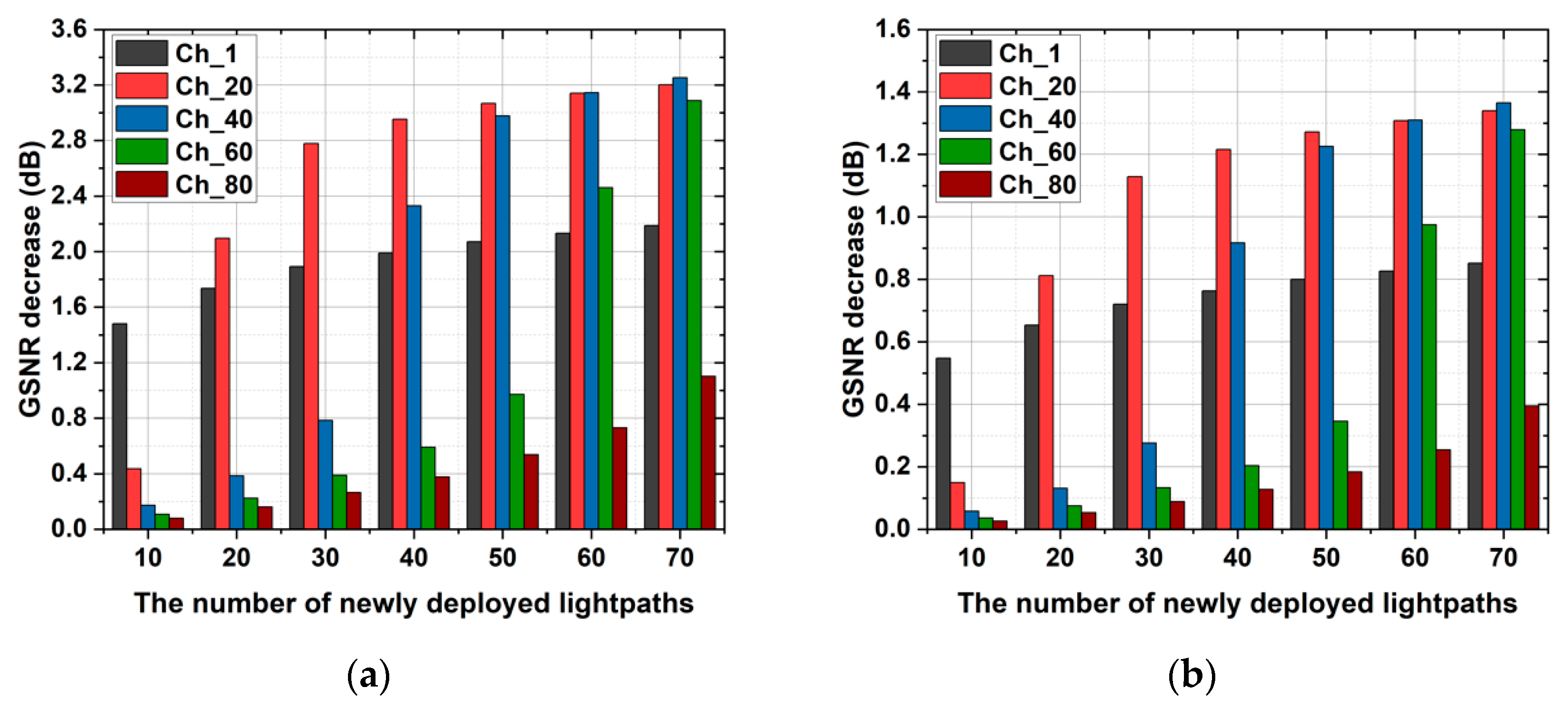
Figure 3a,b show the GSNR decrease of the Ch_1, Ch_20, Ch_40, Ch_60, and Ch_80 caused by the deployment of the new lightpaths in the Jnet and the NSFnet. In the Jnet and the NSFnet, the selected routes are 1-3-5-9-14-13 and 2-4-11-12, respectively, and the wavelength assignment scheme is the first-fit (FF). In
Figure 3a, with the increase in the number of newly deployed lightpaths, the GSNR decrease of the CUTs increases and the maximum GSNR decrease achieves 3.25 dB. Moreover, due to the FF scheme, the GSNR of the channel with the smallest number (Ch_1) decreases the most when the number of newly deployed lightpaths is 10, and when the number of newly deployed lightpaths achieves 70, the GSNR of the channel with the middle number (Ch_40) decreases the most. In
Figure 3b, the performance of the GSNR decrease in the NSFnet is similar to that in the Jnet, and the maximal GSNR decrease of the CUTs is 1.36 dB. The QoT of the previously deployed lightpaths is deteriorated greatly due to the deployment of new lightpaths, and the QoT estimation of the single lightpath cannot capture the decrease in the previously deployed lightpaths’ QoT. Thus, it is necessary to estimate the QoT of new-LPs and pre-LPs simultaneously, i.e., achieve multi-channel QoT estimation, in optical networks.
In this section, we show the performance of the ANN-QoT-E proposed in [
23] and our proposed SA-QoT-E in respect of model convergence, estimation accuracy, scalability, and computational complexity.
4.1. Convergence
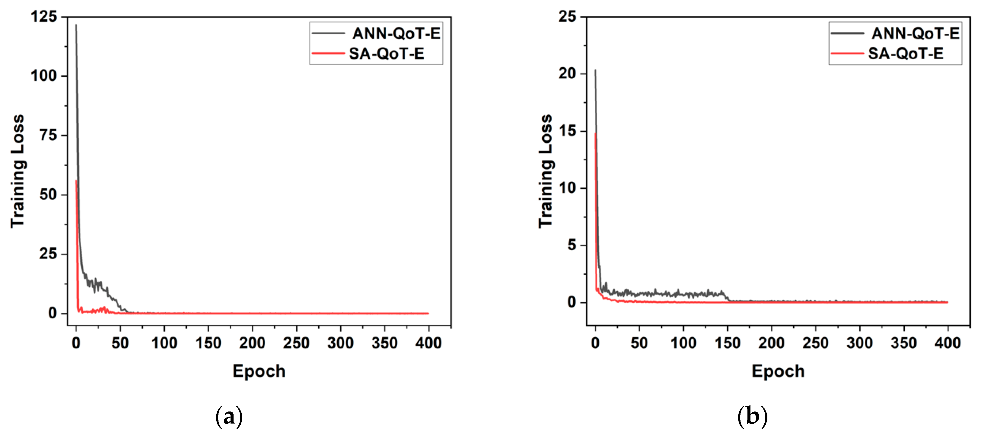
The training processes of the ANN-QoT-E and the SA-QoT-E in the Jnet and NSFnet are shown in
Figure 4a,b. As shown in
Figure 4a, in the Jnet, the ANN-QoT-E and the SA-QoT-E converge after 400 epochs. After 79 epochs, the ANN-QoT-E almost converges and its training loss is 0.127, and the SA-QoT-E almost converges at the 51th epoch and its training loss is 0.127. In
Figure 4b, after 400 epochs, the two models converge in the NSFnet, where the SA-QoT-E almost converges at the 53th epoch with the training loss of 0.059 and the ANN-QoT-E almost converges at 226th epoch with the training loss of 0.057. In conclusion, the SA-QoT-E converges in fewer epochs than the ANN-QoT-E. That is because the SA-QoT-E has a stronger data-fitting ability than the ANN-QoT-E.
4.2. Estimation Accuracy
Figure 5 shows the estimation accuracy of the ANN-QoT-E and the SA-QoT-E tested on the testing dataset.
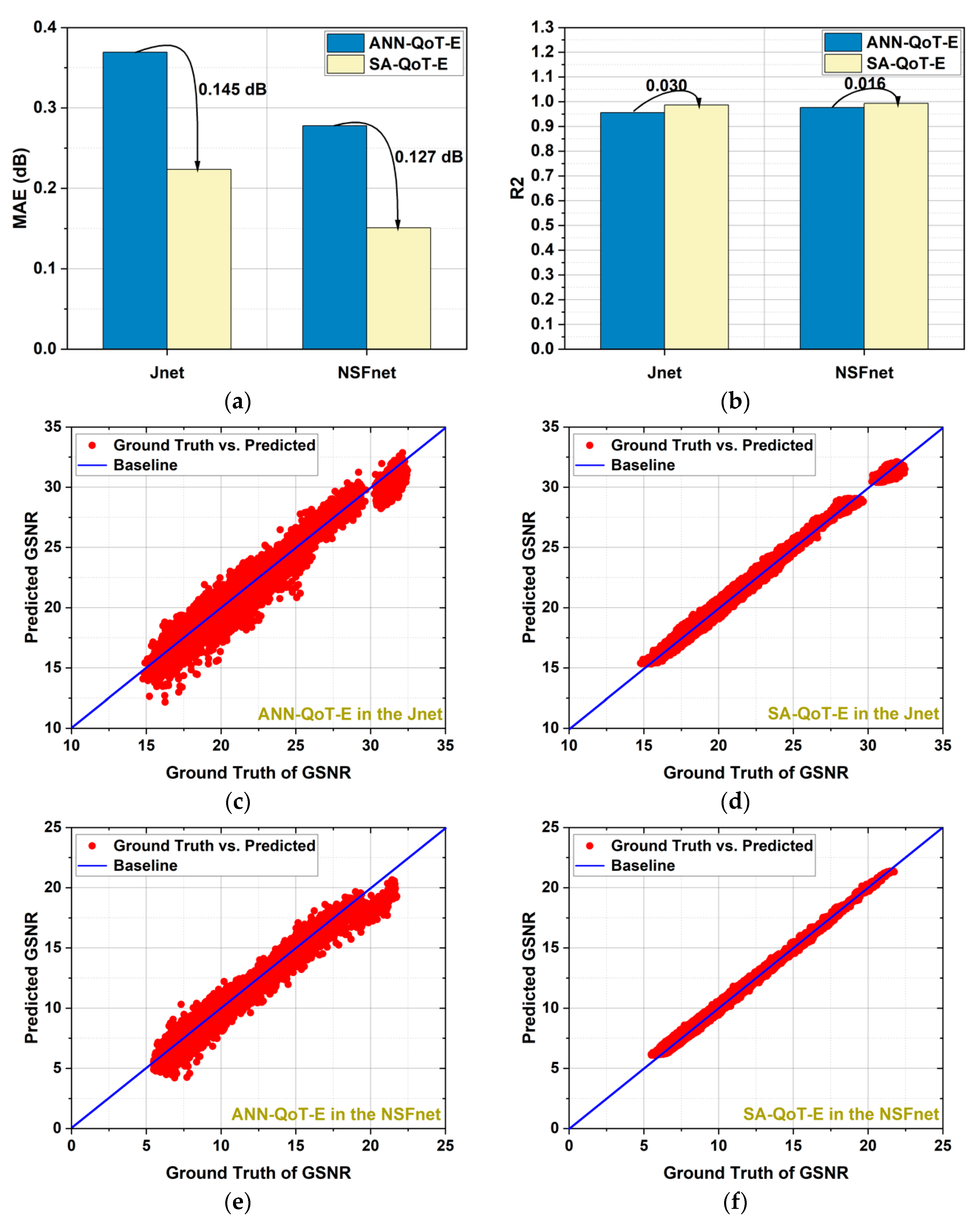
Figure 5a shows the testing of the mean absolute error (MAE) of the two estimation models in the Jnet and NSFnet. The testing MAE of the SA-QoT-E is lower than that of the ANN-QoT-E; specifically, the testing MAE of the SA-QoT-E is 0.147 dB and 0.127 dB lower than that of the ANN-QoT-E in the Jnet and NSFnet, respectively, which means the predicted GSNR of the SA-QoT-E is, on average, 0.147 dB and 0.127 dB closer to the ground truth of the GSNR compared with that of the ANN-QoT-E in the Jnet and NSFnet, respectively. R2 score is a commonly used metric for the evaluation of the regression model, it is closer to 1, and the corresponding model has higher estimation accuracy.
Figure 5b shows that, in the Jnet and the NSFnet, the R2 score of the SA-QoT-E is 0.03 and 0.016 higher than that of the ANN-QoT-E, respectively.
Figure 5c,d show the predicted GSNR of the ANN-QoT-E and the SA-QoT-E against their actual GSNR in the Jnet, respectively. The ideal estimation result is that the scatters distribute on the baseline, which means the predicted GSNR is equal to the actual GSNR. The figures show that, in the Jnet, the estimation accuracy of the SA-QoT-E is higher than that of the ANN-QoT-E; specifically, the maximum absolute error of the SA-QoT-E is 1.13 dB and that of the ANN-QoT-E is 4.21 dB.
Similarly,
Figure 5e,f show the predicted GSNR values of the two models against their actual GSNR in the NSFnet. The results show that the estimation accuracy of the SA-QoT-E is higher than that of the ANN-QoT-E in the NSFnet, where the maximum absolute error of the SA-QoT-E is 0.84 dB and that of the ANN-QoT-E is 3.46 dB.
In the Jnet and the NSFnet, the accuracy of the SA-QoT-E is higher than that of the ANN-QoT-E, which is because the self-attention mechanism assigns weights to the interfering channels according to their effects on the QoT of CUT.
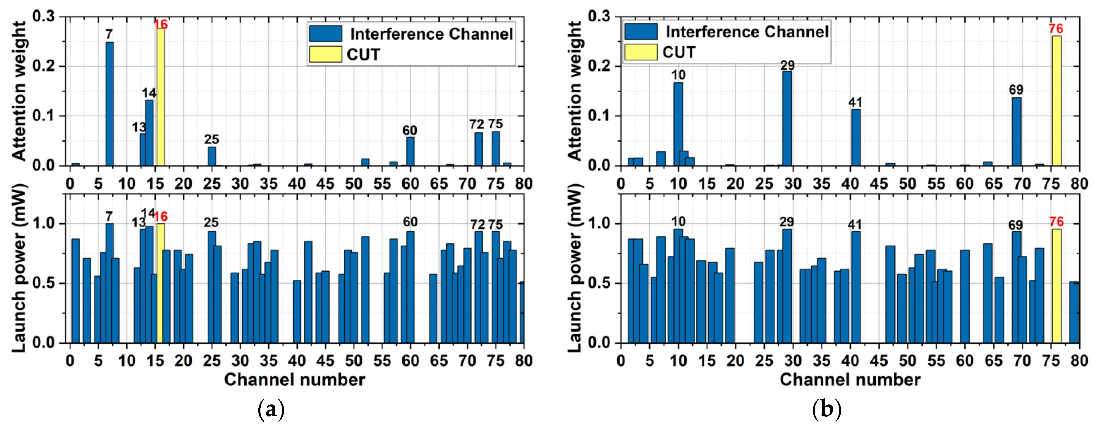
Figure 6a,b show the attention weight and launch power of each channel for Ch_16 in the Jnet and for Ch_76 in the NSFnet, respectively, which is tested by the SA-QoT-E on a randomly selected testing sample. Due to the nonlinear effect of fibers, the interfering channel, which has a higher launch power and closer spectral distance to the CUT (SDC), has a stronger effect on the CUT.
Figure 6a marks the channels with the larger attention weight. In the Jnet, as shown in
Figure 6a, these marked channels are arranged in descending order of attention weight as Ch_16, Ch_7, Ch_14, Ch_75, Ch_72, Ch_13, Ch_60, and Ch_25. The attention weight of Ch_16 is maximal due to its launch power being maximal and SDC being minimal. Though the SDC of Ch_7 is higher than that of Ch_14, the attention weight of Ch_7 is higher than that of Ch_14 due to the higher launch power of Ch_7. The attention weights assigned for Ch_13, Ch_25, Ch_60, Ch_72, and Ch_75 violate the nonlinear effect theory; thus, the accuracy of the SA-QoT-E in the Jnet is lower than that in the NSFnet.
Figure 6b shows that, in the NSFnet, the order of the marked channels according to their attention weight is Ch_76, Ch_29, Ch_10, Ch_69, and Ch_41. The attention weight of Ch_76 is maximal due to the maximal launch power and minimal SDC of Ch_76, and the attention weight of Ch_29 and Ch_10 is higher than that of Ch_69 and Ch_41, which is because the launch power of Ch_29 and Ch_10 is higher than that of Ch_69 and Ch_41. Due to the smaller SDC of Ch_29 than Ch_10, the attention weight of Ch_29 is higher than that of Ch_10. For the same reason, the attention weight of Ch_69 is higher than that of Ch_41. The attention weights assignment in the NSFnet obeys the nonlinear effect theory.
4.3. Scalability
The input dimension and output dimension of ANN models are fixed. When the number of network wavelengths is expanded (such as a C band network expanding to a C+L band network), the original ANN-QoT-E cannot be applied to the network. The SA-QoT-E has the advantage of variable length of the input feature vector sequence due to the introduction of the self-attention mechanism. We generate new testing datasets in the Jnet with 120 wavelengths (the full channels of the C++ band), in the Jnet with 216 wavelengths (the full channels of the C+L band), in the NSFnet with 120 wavelengths, and in the NSFnet with 216 wavelengths, which are defined as
,
,
, and
, respectively.
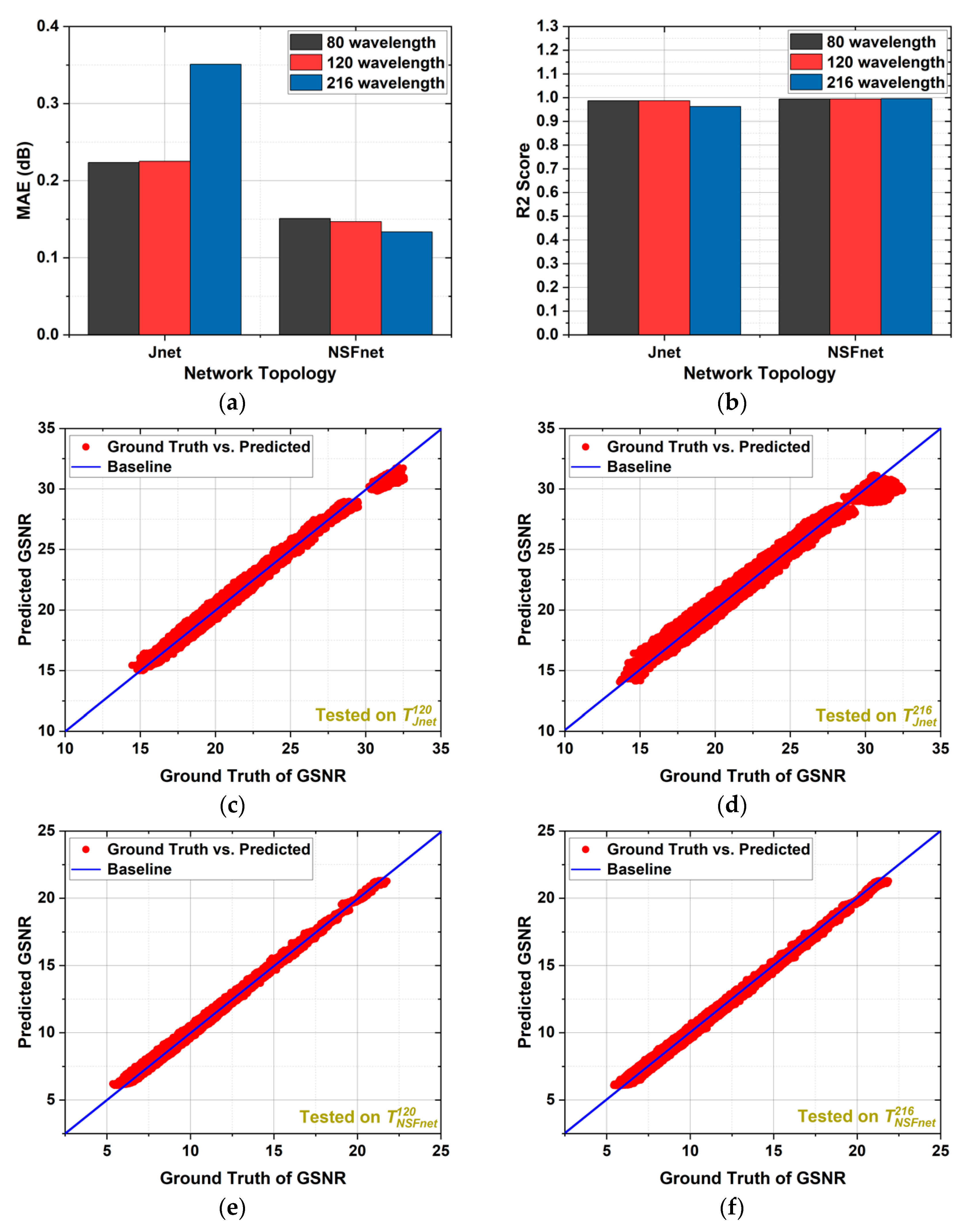
Figure 7 shows the estimation accuracy of the SA-QoT-E in the Jnet and NSFnet obtained by testing on
/
/
and
/
/
, where the SA-QoT-E is trained on
/
. As shown in
Figure 7a, in the Jnet, the testing MAEs of the SA-QoT-E tested on
/
/
are low; even the highest MAE obtained on
is lower than the MAE obtained by the ANN-QoT-E in
Figure 5a; in the NSFnet, the testing MAEs of the SA-QoT-E tested on
/
/
are close and low.
Figure 7b shows the R2 score of the SA-QoT-E tested on
/
/
and
/
/
, in the Jnet and NSFnet, and the SA-QoT-E achieves a high R2 score.
Figure 7c,d show the predicted value of the SA-QoT-E against their actual GSNR tested on
and
, respectively. The results show that the SA-QoT-E trained on
has a relatively high accuracy on
and
; specifically, the maximum absolute errors of the SA-QoT-E tested on
and
are 1.79 dB and 2.58 dB, respectively.
Figure 7e,f show that the SA-QoT-E trained on
has a relatively high accuracy on
and
; specifically, the maximum absolute errors of the SA-QoT-E tested on
and
are 0.84 dB and 0.73 dB, respectively.
The self-attention mechanism learns the interaction between channels, and aggregates multiple channel feature vectors into a new channel feature vector to estimate the QoT of the corresponding channel, Thus, the SA-QoT-E is not limited by the number of network channels. In conclusion, the SA-QoT-E can be directly applied to network wavelength expansion scenarios without retraining.
4.4. Computational Complexity
Compared with the ANN-QoT-E, the SA-QoT-E not only improves the estimation accuracy but also has scalability. However, the SA-QoT-E has higher computational complexity. The computational complexity is the total number of addition operations and multiplication operations of the QoT estimators. The computational complexity of each layer of the ANN models is its input dimension multiplied by its output dimension; thus, the computational complexity of the ANN-QoT-E in our simulations can be calculated as follows:
where
is the computational complexity of the ANN-QoT-E,
is the number of wavelengths in the network, and
is the number of neurons in the ANN model’s hidden layer.
The self-attention mechanism mainly contains three steps: (1) similarity calculation; (2) soft-max operation; (3) weighted summation. First, the computational complexity of the similarity calculation is
, due to the fact that it is a
matrix multiplied by a
matrix. In addition, the computational complexity of soft-max operation is
. Finally, the weighted summation is a
matrix multiplied by a
matrix; thus, its computational complexity is
. The computational complexity of the ANN model in the SA-QoT-E is
. Therefore, the computational complexity of the SA-QoT-E is shown as follows:
where
is the computational complexity of the SA-QoT-E. The computational complexity of the ANN-QoT-E and the SA-QoT-E is shown in
Table 2. Obviously, the computational complexity of the SA-QoT-E is higher than that of the ANN-QoT-E. However, the training of the estimation models is offline and
is acceptable, and the SA-QoT-E can be applied to realistic optical network optimization.
4.5. Discussion
The estimation accuracy of QoT estimators is important to ensure the reliable transmission of the lightpaths in optical networks, and the computational complexity of QoT estimators decides their availability in practical scenarios. The SA-QoT-E has the advantages compared with the ANN-QoT-E: (1) stronger data-fitting ability; (2) higher estimation accuracy; (3) stronger scalability. However, these advantages of SA-QoT-E come at the cost of high computational complexity. The computational complexity of SA-QoT-E is higher than that of the ANN-QoT-E, which is mainly affected by the number of channels . Thus, the ANN-QoT-E is more suitable for optical networks with a large number of network channels and a shortage of computing resources. In most scenarios, the SA-QoT-E has more advantages compared with the ANN-QoT-E.
5. Conclusions
In multi-channel optical networks, due to the nonlinear effect of fibers, the different interfering channel has a different effect on the CUT. The existing ANN-QoT-E ignores the different effects of the interfering channels, which affects its estimation accuracy. To improve the accuracy of the ANN-QoT-E, we propose a novel SA-QoT-E, where the self-attention mechanism assigns attention weights to the interfering channels according to their effects on the CUT. Moreover, we use a hyperparameter search method to optimize the hyperparameters of the SA-QoT-E. The simulation results show that the proposed SA-QoT-E improves the estimation accuracy compared with the ANN-QoT-E. Specifically, compared with the ANN-QoT-E, the testing MAE achieved by the SA-QoT-E is decreased by 0.147 dB and 0.127 dB in the Jnet and NSFnet, respectively; the R2 score achieved by the SA-QoT-E is improved by 0.03 and 0.016 in the Jnet and NSFnet, respectively; the maximal absolute error achieved by the SA-QoT-E is reduced from 4.21 dB to 1.13 dB in the Jnet and from 3.46 dB to 0.84 dB in the NSFnet. Moreover, the SA-QoT-E has scalability, which can be directly applied to network wavelength expansion scenarios without retraining. However, compared with the ANN-QoT-E, the SA-QoT-E has higher computational complexity. Fortunately, the training of the SA-QoT-E is offline and the computational complexity of the SA-QoT-E is acceptable; thus, the proposed SA-QoT-E can be applied to the realistic optical network and provide more accurate lightpath QoT information for optical network optimization.

 and
and 


