Flat-Top Focal Spot and Polarization Conversion Obtained in Tightly Focused Circularly Polarized Light


Abstract
:1. Introduction
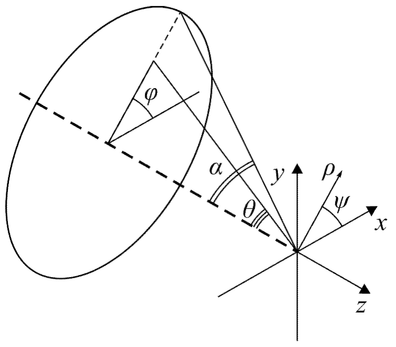
2. Methods
3. Results
3.1. Numerical Simulation of Light Focusing by a Planar Diffractive Lens
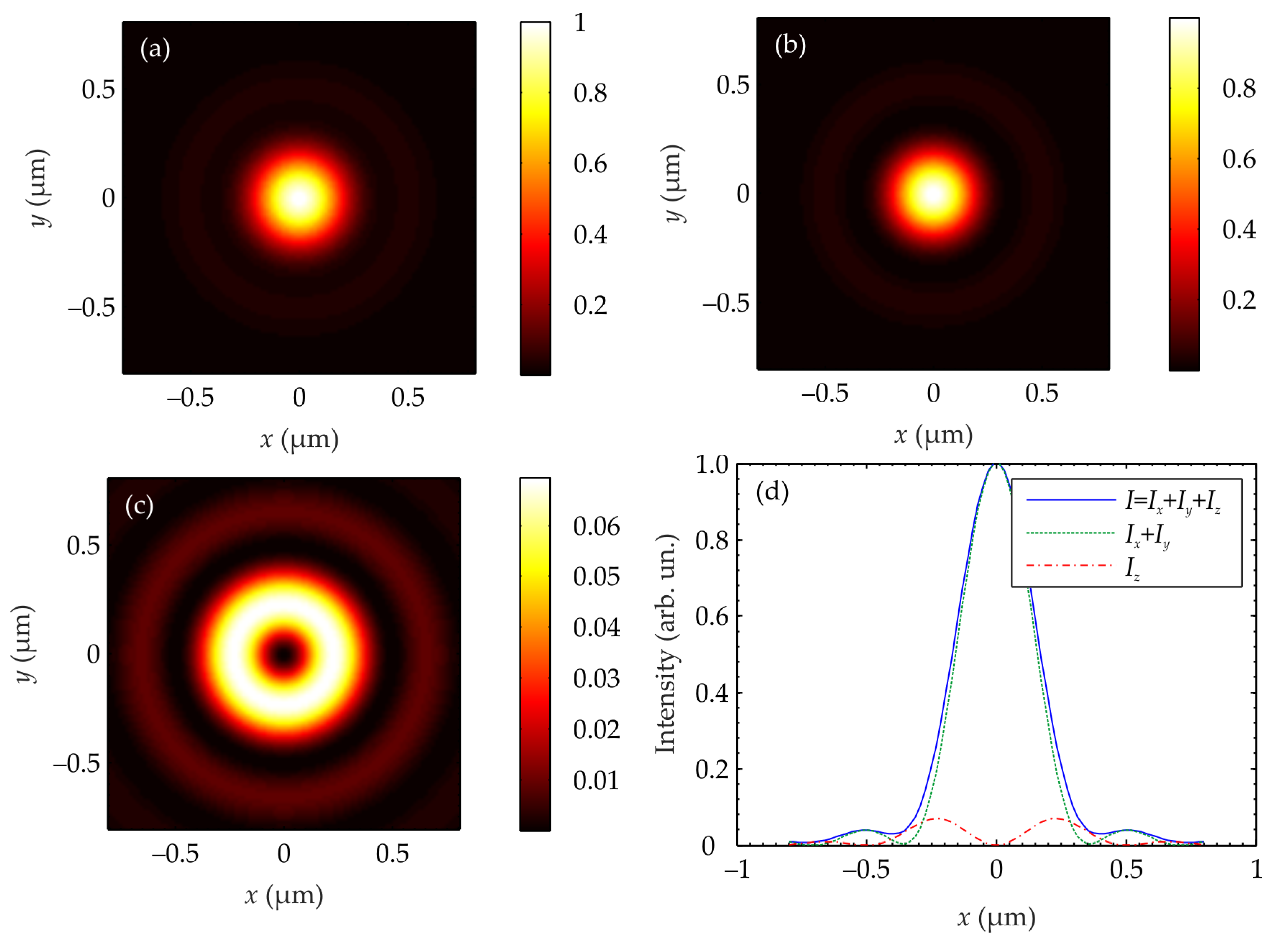
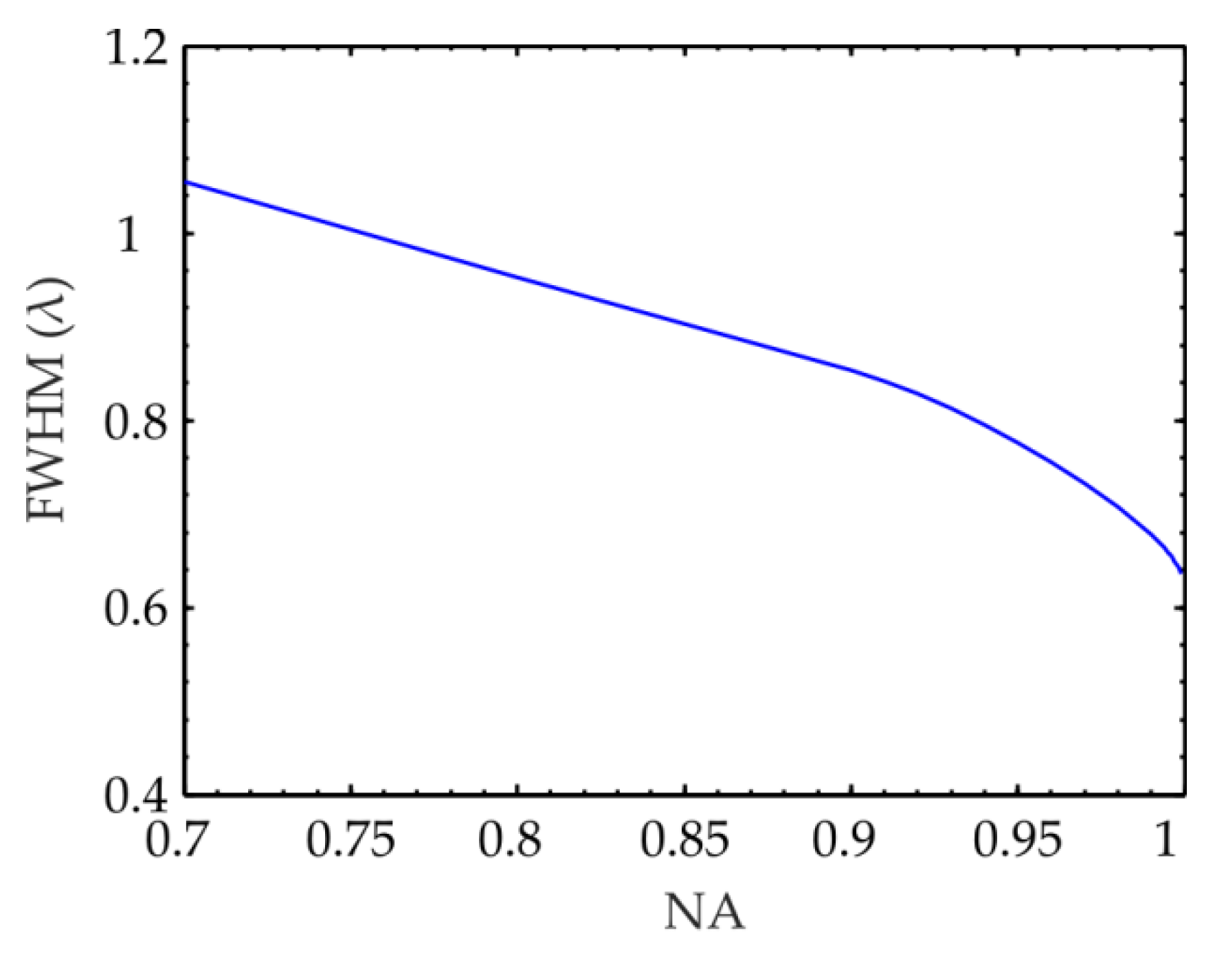
3.2. Numerical Simulation of Light Focusing with an Aplanatic Lens
3.3. Polarization near the Sharp Focus
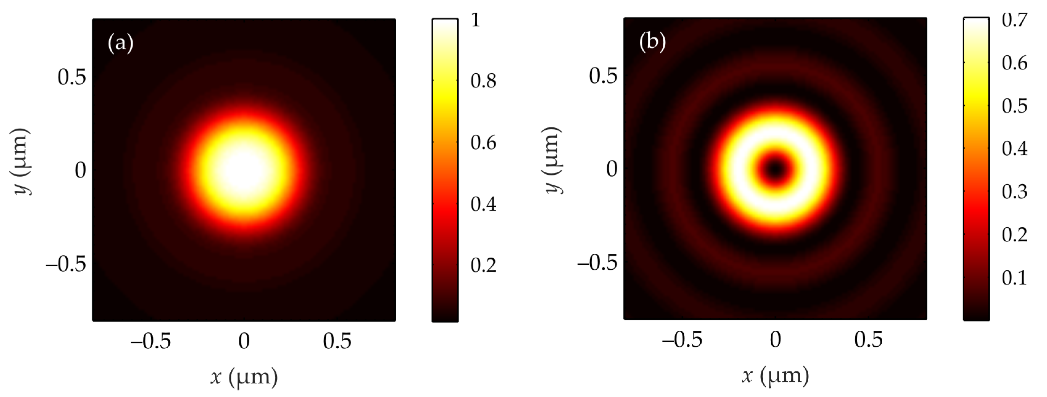
3.4. Focusing Optical Vortex with Circular Polarization
4. Conclusions
Author Contributions
Funding
Institutional Review Board Statement
Informed Consent Statement
Data Availability Statement
Conflicts of Interest
References
- Man, Z.; Dou, X.; Urbach, H.P. The evolutions of spin density and energy flux of strongly focused standard full Poincaré beams. Opt. Commun. 2020, 458, 124790. [Google Scholar] [CrossRef]
- Man, Z.; Bai, Z.; Zhang, S.; Li, X.; Li, J.; Ge, X.; Zhang, Y.; Fu, S. Redistributing the energy flow of a tightly focused radially polarized optical field by designing phase masks. Opt. Express 2018, 26, 23935. [Google Scholar] [CrossRef] [PubMed]
- Gao, X.-Z.; Pan, Y.; Zhang, G.-L.; Zhao, M.-D.; Ren, Z.-C.; Tu, C.-G.; Li, Y.-N.; Wang, H.-T. Redistributing the energy flow of tightly focused ellipticity-variant vector optical fields. Photonics Res. 2017, 5, 640. [Google Scholar] [CrossRef]
- Jiao, X.; Liu, S.; Wang, Q.; Gan, X.; Li, P.; Zhao, J. Redistributing energy flow and polarization of a focused azimuthally polarized beam with rotationally symmetric sector-shaped obstacles. Opt. Lett. 2012, 37, 1041. [Google Scholar] [CrossRef] [PubMed]
- Richards, B.; Wolf, E. Electromagnetic Diffraction in Optical Systems. II. Structure of the Image Field in an Aplanatic System. Proc. R. Soc. A Math. Phys. Eng. Sci. 1959, 253, 358–379. [Google Scholar]
- Stafeev, S.S.; Nalimov, A.G.; Kovalev, A.A.; Zaitsev, V.D.; Kotlyar, V.V. Circular Polarization near the Tight Focus of Linearly Polarized Light. Photonics 2022, 9, 196. [Google Scholar] [CrossRef]
- Bauer, T.; Banzer, P.; Karimi, E.; Orlov, S.; Rubano, A.; Marrucci, L.; Santamato, E.; Boyd, R.W.; Leuchs, G. Observation of optical polarization Möbius strips. Science 2015, 347, 964–966. [Google Scholar] [CrossRef]
- Wang, H.; Shi, L.; Lukyanchuk, B.; Sheppard, C.; Chong, C.T. Creation of a needle of longitudinally polarized light in vacuum using binary optics. Nat. Photonics 2008, 2, 501–505. [Google Scholar] [CrossRef]
- Dorn, R.; Quabis, S.; Leuchs, G. Sharper Focus for a Radially Polarized Light Beam. Phys. Rev. Lett. 2003, 91, 233901. [Google Scholar] [CrossRef]
- Grosjean, T.; Gauthier, I. Longitudinally polarized electric and magnetic optical nano-needles of ultra high lengths. Opt. Commun. 2013, 294, 333–337. [Google Scholar] [CrossRef]
- Wang, X.; Zhu, B.; Dong, Y.; Wang, S.; Zhu, Z.; Bo, F.; Li, X. Generation of equilateral-polygon-like flat-top focus by tightly focusing radially polarized beams superposed with off-axis vortex arrays. Opt. Express 2017, 25, 26844–26852. [Google Scholar] [CrossRef] [PubMed]
- Ping, C.; Liang, C.; Wang, F.; Cai, Y. Radially polarized multi-Gaussian Schell-model beam and its tight focusing properties. Opt. Express 2017, 25, 32475–32490. [Google Scholar] [CrossRef]
- Chen, H.; Tripathi, S.; Toussaint, K.C. Demonstration of flat-top focusing under radial polarization illumination. Opt. Lett. 2014, 39, 834–837. [Google Scholar] [CrossRef] [PubMed]
- Kasinski, J.J.; Burnham, R.L. Near-diffraction-limited laser beam shaping with diamond-turned aspheric optics. Opt. Lett. 1997, 22, 1062. [Google Scholar] [CrossRef]
- Li, Y. Light beams with flat-topped profiles. Opt. Lett. 2002, 27, 1007. [Google Scholar] [CrossRef]
- Eyyuboglu, H.T.; Arpali, Ç.; Baykal, Y.K. Flat topped beams and their characteristics in turbulent media. Opt. Express 2006, 14, 4196. [Google Scholar] [CrossRef]
- Kotlyar, V.V.; Nalimov, A.G.; Stafeev, S.S. Exploiting the circular polarization of light to obtain a spiral energy flow at the subwavelength focus. J. Opt. Soc. Am. B 2019, 36, 2850–2855. [Google Scholar] [CrossRef]
- Stafeev, S.S.; Zaitsev, V.D.; Kotlyar, V.V. Circular polarization before and after the sharp focus for linearly polarized light. Comput. Opt. 2022, 46, 381–387. [Google Scholar] [CrossRef]
- Davidson, N.; Bokor, N. High-numerical-aperture focusing of radially polarized doughnut beams with a parabolic mirror and a flat diffractive lens. Opt. Lett. 2004, 29, 1318–1320. [Google Scholar] [CrossRef]
- Stafeev, S.S.; Zaicev, V.D. A minimal subwavelength focal spot for the energy flux. Comput. Opt. 2021, 45, 685–691. [Google Scholar] [CrossRef]
- Stafeev, S.S.; Nalimov, A.G. Longitudinal component of the Poynting vector of a tightly focused optical vortex with circular polarization. Comput. Opt. 2018, 42, 190–196. [Google Scholar] [CrossRef]


Disclaimer/Publisher’s Note: The statements, opinions and data contained in all publications are solely those of the individual author(s) and contributor(s) and not of MDPI and/or the editor(s). MDPI and/or the editor(s) disclaim responsibility for any injury to people or property resulting from any ideas, methods, instructions or products referred to in the content. |
© 2022 by the authors. Licensee MDPI, Basel, Switzerland. This article is an open access article distributed under the terms and conditions of the Creative Commons Attribution (CC BY) license (https://creativecommons.org/licenses/by/4.0/).
Share and Cite
Stafeev, S.S.; Zaitsev, V.D.; Kotlyar, V.V. Flat-Top Focal Spot and Polarization Conversion Obtained in Tightly Focused Circularly Polarized Light. Photonics 2023, 10, 32. https://doi.org/10.3390/photonics10010032
Stafeev SS, Zaitsev VD, Kotlyar VV. Flat-Top Focal Spot and Polarization Conversion Obtained in Tightly Focused Circularly Polarized Light. Photonics. 2023; 10(1):32. https://doi.org/10.3390/photonics10010032
Chicago/Turabian StyleStafeev, Sergey S., Vladislav D. Zaitsev, and Victor V. Kotlyar. 2023. "Flat-Top Focal Spot and Polarization Conversion Obtained in Tightly Focused Circularly Polarized Light" Photonics 10, no. 1: 32. https://doi.org/10.3390/photonics10010032