Article

Critical Laser Intensity of Phase-Matched High-Order Harmonic Generation in Noble Gases

1
Theoretisch-Physikalisches Institut, Friedrich-Schiller-Universität Jena, Fürstengraben 1, 07743 Jena, Germany
2
Helmholtz Institute Jena, Fröbelstieg 3, 07743 Jena, Germany
3
GSI Helmholtzzentrum für Schwerionenforschung GmbH, Planckstraße 1, 64291 Darmstadt, Germany
4
Institute of Applied Physics, Abbe Center of Photonics, Friedrich Schiller University Jena, Albert-Einstein-Str. 15, 07745 Jena, Germany
5
Fraunhofer Institute for Applied Optics and Precision Engineering, Albert-Einstein-Str. 7, 07745 Jena, Germany
*
Author to whom correspondence should be addressed.
Photonics 2023, 10(1), 24; https://doi.org/10.3390/photonics10010024
Submission received: 18 November 2022 / Revised: 19 December 2022 / Accepted: 20 December 2022 / Published: 26 December 2022

Abstract

:
The efficient generation of high-order harmonic radiation has been a challenging task since the early days of strong-field physics. An essential requirement to achieve efficient high-order harmonic generation inside a gas medium is the phase matching of the high-order harmonic radiation and the incident laser pulse. The dominant contribution to the wave–vector mismatch Δ k is associated with the ionization probability of the medium. In this work, we derive two analytical formulas to calculate the critical intensity of a general linearly polarized laser pulse that obey the phase-matching condition Δ k = 0 . The analytic formulas are valid in the tunneling regime (ADK model) and the regime of the tunnel and multi-photon ionization (PPT model), respectively. We compare our results to numerical computations and discuss the scaling of the critical intensity depending on the pulse duration and the wavelength of a realistic incident laser pulse. The analytical approach demonstrated in this work is highly accurate and can compete with the existing numerical computational methods by an error of less than 1% and a decrease in the computation time of approximately 4 to 6 orders of magnitude. This enables complex theoretical studies of the efficiency scaling in HHG or to consider the effects of ground state depletion efficiently.

1. Introduction

High-order harmonic generation (HHG) is an essential technique to produce coherent ultra-short light pulses from tabletop-sized devices. The radiation from these devices can be used in industry and in fundamental scientific research, which highlights them as a promising source for a broad range of applications.
The macroscopic conversion efficiency of the high-order harmonic (HH) process is on the order of 10 4 at 30 eV [1] down to 10 9 at 300 eV [2]. Specifically, the conversion efficiency of HHG from near- to mid-infrared laser pulses decreases exponentially with increasing wavelengths, which has been demonstrated in experimental and theoretical work [3,4,5]. This low efficiency induced the interest of the strong-field community to find specific experimental conditions that optimize the HH yield [6,7,8,9,10]. The highest experimental conversion efficiencies can be achieved by simultaneously optimizing macroscopic effects such as absorption [11], laser focusing [12,13], and phase matching [14,15,16].
Phase matching (PM) is one of the essential requirements to efficiently produce HH radiation. Therefore, the phase velocity of the incident laser pulse and the generated HH radiation need to match while propagating through the gas medium. The PM of complex pulse structures, e.g., twisted light [16,17], is often relatively complicated; thus, linearly polarized laser pulses are advantageous to simplify the PM. Commonly used media for the generation of HH radiation are isotropic noble gases, which are also the focus of this work. The conventional approach of second or third-order harmonic generation of using birefringence to phase-match the fundamental and harmonic beam cannot be used. However, it can be shown that the contribution of plasma (free electrons + ions) and neutral gas dispersion, the geometrical phase, and the intrinsic phase can be balanced to achieve a transient phase-matching window [14].
In this work, we analytically investigate the PM conditions for a partially ionized noble gas in the free-focusing regime that can be generalized to other geometries (e.g., tight focusing or waveguide). We explicitly show that the critical peak intensity of a realistic laser pulse depends inverse logarithmically on the pulse duration and, further, has a nontrivial wavelength dependency associated with the refraction index. In the discussed experimental setup, other PM contributions are nullified by each other. That enables us to discuss an experimental setup under realistic conditions and demonstrate a newly developed calculation technique. However, this calculation technique is not limited to a specific experimental setup and may be adapted, e.g., in complex analytical or numerical studies, where a numerically calculated ionization rate is not suited.
This paper is structured as follows: In Section 2, we derive the analytical formulas of the critical field intensities for which PM is achieved at the peak of the incident laser pulse. In more detail, in Section 2.1, we revisit the standard model of PM for HHG and specify the PM condition of this work. In Section 2.2, we derive and discuss the formula of the critical intensity in the tunneling regime. Section 2.3 generalizes the derived formula to the intermediate regime where the tunnel and multi-photon ionization needs to be considered, which incorporates many realistic scenarios. In Section 3, we compare our results with numerical calculations and discuss the parameter range for which the developed method is valid. Finally, we conclude our findings in Section 4. In the following, we use atomic units ( = e = m e = 4 π ϵ 0 = 1 ) unless stated otherwise.

2. Model and Method

In Figure 1, we can see a standard HHG setup with the incident laser pulse on the left (orange-red) and the emitted HH radiation on the right (blue). This work focuses on the linear propagation effects of the HH radiation and the incident laser pulse inside the gas medium. In particular, we focus on the phase-matching of these light fields, which is highlighted in Figure 1a by the dashed circle.
The medium consists of an arbitrary noble gas characterized by its ionization potential I p and orbital angular momentum quantum number of the respective atomic state. We assume that the incident laser pulse is a paraxial linearly polarized plane wave propagating in the z-direction (optical axis) that irradiates the gas target (free-focusing regime). The optical axis is perpendicular to the target surface in the x-y plane while the target is centered one Rayleigh range behind the focus of the incident laser pulse z = z R (not explicitly shown in Figure 1a). Experimentally, this is done to favor the phase-matched generation of the short trajectories [18]. In the free-focusing regime, the variation of the electric field strength on the optical axis can be neglected for gas targets that are much thinner than the Rayleigh range such that the atoms in the interaction region are affected by a constant field strength. In the following Section 2.1, we use the SI unit system.

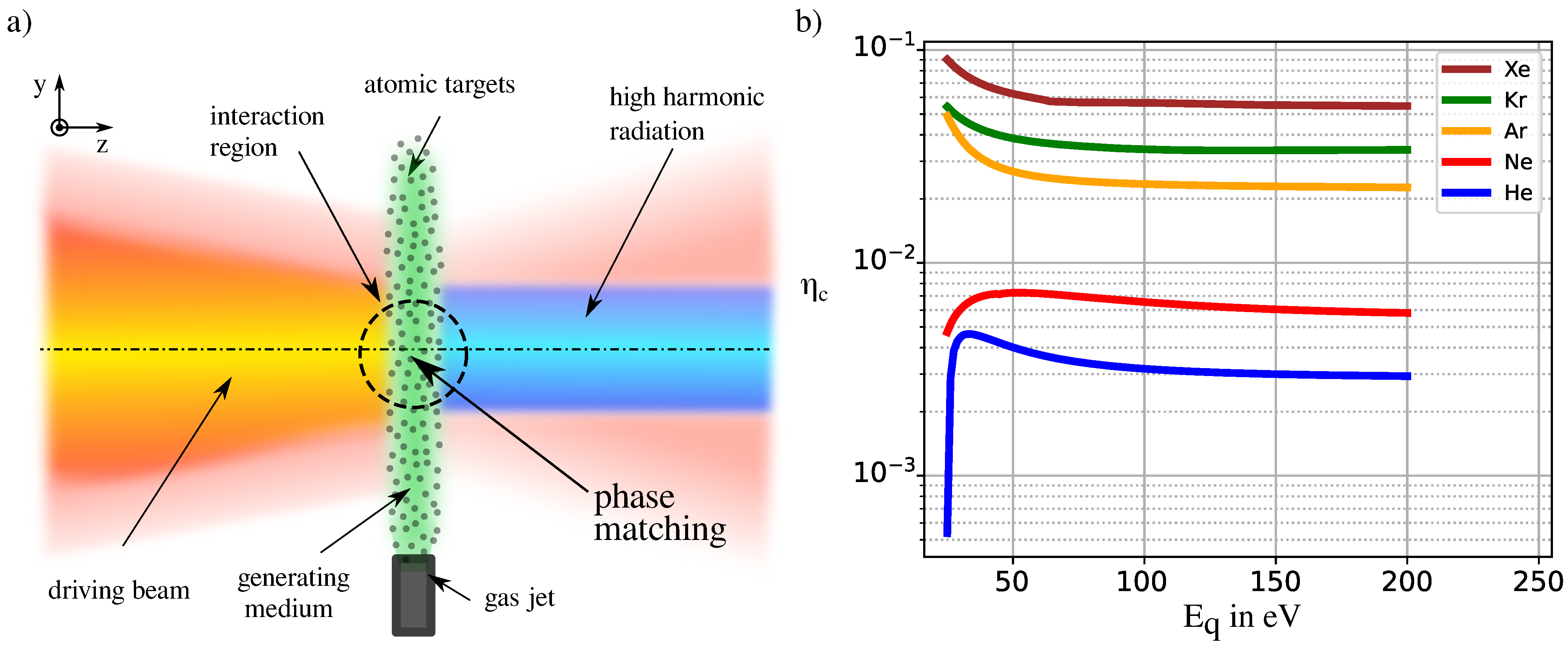
2.1. Phase Matching of High-Order Harmonic Radiation

For a coherent build-up of the HH radiation, the wave–vector mismatch has to be minimized, resulting in efficient HHG. The wave–vector mismatch is defined as
Δ k = k ( q ω ) q k ( ω ) ,
where the first term is associated with the HH radiation and the second with the incident laser pulse. The wave–vector mismatch consists of four major contributions in the free-focusing regime, as discussed in [19]
Δ k = Δ k a t o m + Δ k p l a s m a + Δ k G o u y + Δ k i n t r i n s i c 0 ,
where Δ k a t o m and Δ k p l a s m a consider the mismatch associated with the neutral and ionized atoms, respectively. The term Δ k G o u y , on the other hand, denotes a geometric contribution by the Gouy phase, and Δ k i n t r i n s i c describes the wave–vector mismatch related to the intrinsic phase of the emitted photons. The Gouy wave–vector mismatch has a positive contribution, whereas the intrinsic phase results in a negative contribution to the total wave–vector mismatch. These two contributions nullify; eventually Δ k G o u y + Δ k i n t r i n s i c 0 , as the target is centered one Rayleigh length behind the focus of the laser pulse [18,20,21]. This leaves us with the atomic and plasma contributions that can be combined to an dispersion mismatch as
Δ k d i s p = Δ k a t o m + Δ k p l a s m a , q ω c 0 ρ N a t m Δ δ 1 η η c = 0 ,
where ω is the frequency of the laser pulse, c 0 is the speed of light in the vacuum, N a t m is the particle number at standard conditions, ρ is the particle density, and Δ δ = n 0 ( ω ) n 0 ( q ω ) is the difference between the refractive indices of the laser pulse and the qth harmonic under standard conditions. The respective refraction indices are calculated as in [22,23,24]. The ionization probability η denotes macroscopically the relative amount of atoms in an ionized state compared to the total number of atoms. Furthermore, η c is the so-called critical ionization probability that is defined as
η c = 1 + 2 π r e N a t m c 0 2 ω 2 Δ δ 1 ,
where r e = e 2 / 4 π ϵ 0 m e c 0 2 is the classical electron radius. To fulfill (3), the term inside the parentheses should vanish, which is fulfilled if the ionization probability matches the critical ionization probability η = η c in Equation (3). The critical ionization probability (4) of commonly used noble gases is shown in Figure 1b for a fundamental laser wavelength of λ = 1000 nm .

2.2. ADK Model: Critical Field Intensity

In this work, we investigate strong-field ionization in the context of phase-matched high-order harmonic generation. Apart from solving the time-dependent Schrödinger equation numerically, the YI model [25] does describe the strong-field ionization sufficiently well. As HHG is known to operate in the regime of tunnel and multi-photon ionization, we restrict our investigations to approximations of the YI model that incorporate the respective ionization processes (ADK and PPT).
This section is separated into two parts. In the first part, we sketch the idea of a solution that obeys Equation (3). The second part incorporates a detailed derivation as well as a discussion of the applied approximations.

2.2.1. Critical Field Intensity as Phase Matching Condition

For a pulsed laser, it is impossible to fulfill Equation (3) in general because the ionization probability increases monotonically over time. Therefore, the PM condition should be achieved at the peak of the laser pulse, resulting in the highest number of ionized electrons. The ADK ionization rate is defined as [20,26]
w A D K ( t ) = 1 ( 2 + 1 ) m = w m A D K ( t ) , = m = | C n * l * | 2 G l m I p ( 2 + 1 ) 2 ( 2 I p ) 3 / 2 F ( t ) 2 n * | m | 1 e 2 ( 2 I p ) 3 / 2 3 F ( t ) , m = κ m F 0 F ( t ) g m + 1 e F 0 F ( t ) ,
with the atomic species dependent factor κ m = 3 g m + 1 | C n * l * | 2 G l m I p ( 2 + 1 ) 1 , which defines the time-independent amplitude of the ionization rate concerning the initial state of the ionized electron. The parameters | C n * l * | 2 and G l m are defined in Equations (4.65) and (4.66) in [20], respectively. Moreover, we define the terms
F 0 = 2 3 ( 2 I p ) 3 2 , and g m = 2 n * | m | 2 ,
as atom-specific constants, and the electric field of the laser pulse reads
F ( t ) = E 0 f ( t ) cos ( ω t ) ,
f ( t ) = e 4 ln ( 2 ) t τ 2 .
Here, f ( t ) denotes a Gaussian envelope with a full-width half maximum pulse duration of τ . The ADK ionization probability in the peak of the laser pulse then reads [20]
η = η A D K = 1 e 0 w A D K ( t ) d t .
One can see the dependency of the ionization probability on the laser frequency ω , the atomic ionization potential I p , the pulse duration τ , and the peak intensity of the laser pulse I = E 0 . In the experimental setup, it is often not possible to adapt the atomic species or the wavelength of the laser pulse to optimize these parameters with regard to the PM condition (3). On the other hand, the intensity and the pulse duration can be controlled relatively easily compared to other parameters. Following this idea, we can define the critical intensity I c of the laser pulse as a function of the wavelength, atomic species, and pulse duration that fulfills (3) with
η ( I , τ , I p , λ ) = η c η ( I c ( τ , I p , λ ) ) = η c .
Numerical algorithms are often used to find the critical intensity I c from Equation (9) that fulfills the phase matching condition in Equation (3). These algorithms integrate the ADK ionization rate in Equation (5) (or PPT rate in (25)) for a given intensity and iteratively optimize them until the intensity converges to the critical intensity I = I c . In other words, these algorithms have the temporal integration of Equation (9) inside a root-finding algorithm. This algorithm can be computationally heavy because the numerical integration needs to be executed for each iteration of the root-finding algorithm.
Within our analytical approach, which is in detail derived in Section 2.2.2, the critical intensity of the ADK model I c I c ( 0 ) is approximated by
I c ( 0 ) ( τ , I p , λ ) = g 0 F 0 W 0 1 g 0 D 0 τ 1 / g 0 2 , for g 0 < 0 ,
I c ( 0 ) ( τ , I p , λ ) = g 0 F 0 W 1 1 g 0 D 0 τ 1 / g 0 2 , for g 0 > 0 ,
D 0 = 2 2 ln ( 2 ) | ln ( 1 η c ) | κ 0 .
where κ m is defined below Equation (5) and g 0 in Equation (6) with m 0 . The Lambert W function is denoted by W i for its respective real branch with i { 0 , 1 } . For all neutral noble gases, except Xenon, the parameter g 0 is smaller than zero such that Equation (11) can be used for helium, neon, argon, and krypton, whereas Equation (12) can be used for xenon. Note that the variables F 0 and g 0 depend only on the atomic species, whereas D 0 ln ( 1 η c ( λ ) ) depends on the wavelength of the incident laser pulse. The dependency of the critical intensity on the laser pulse is therefore imprinted in the critical ionization probability η c η c ( λ ) and the pulse duration τ . The atomic-species dependent parameters for the noble gases can be found in Table 1.
| ln ( 1 η c ( λ 0 ) ) | τ 0 = | ln ( 1 η c 0 ) | τ 0 | ln ( 1 η c 1 ) | τ 1 τ 1 = τ 0 | ln ( 1 η c 1 ) | | ln ( 1 η c 0 ) | τ 0 η c 1 η c 0 for η c 0 , η c 1 < < 1
Equation (14) denotes a condition for the pulse duration τ 1 in which the critical intensity of the incident laser pulse remains invariant while changing the parameters from λ 0 , τ 0 λ 1 , τ 1 . The factor | ln ( 1 η c ) | is physically equivalent to the time-integrated ionization rate at the peak of the laser pulse
| ln ( 1 η c ) | = 0 d t w A D K ( t ) .
If we reformulate Equation (14), we can find the following invariance relation:
The critical field intensity is invariant under a parameter change from ( τ 0 , λ 0 ) to ( τ 1 , λ 1 ) , if the relative time integrated ionization rate equals the relative pulse duration.
τ 1 τ 0 = n 1 λ 1 n 0 λ 0 = ln ( 1 η c ( λ 1 ) ) ln ( 1 η c ( λ 0 ) ) = ln ( 1 η c 1 ) ln ( 1 η c 0 ) and if η c 1 , η c 0 < < 1 τ 1 τ 0 η c 1 η c 0
Simplifying (11) and (12) even further reveals a simple scaling law of the critical intensity for both positive and negative g 0 [27].
I c ( 0 ) ( τ , I p , λ ) g 0 F 0 ln 1 | g 0 | D 0 τ 1 / | g 0 | 2 F 0 2 ln 2 D 0 τ I c ( 0 ) ( τ ) ln 2 | ln ( 1 η c ) | τ
With this fairly simple scaling law, we are able to describe the general proportionality of the critical intensity for all noble gases with respect to the pulse duration and the critical ionization probability of a monochromatic Gaussian laser pulse.
To summarize, the critical intensity calculated in (11) depends on the incident laser pulse via the pulse duration τ and, indirectly, on the wavelength of the laser pulse η c ( λ ) , where it obeys the proportionality I c ( 0 ) ln 2 ( | ln ( 1 η c ) | τ ) . The wavelength dependency is directly related to the critical ionization probability in which the refractive index is sensitive to the wavelength of the incident laser pulse. The critical intensity does not significantly depend on electrons ionized from states with the magnetic quantum number m = ± 1 . At the same time, the dependency on the ionization potential I p cannot be derived so easily.

2.2.2. Derivation of the Critical Intensity

In the following derivation, we make use of a number of approximations. All of these approximations can be reduced to one of the following major assumptions.
  • F 0 / E 0 > > 1 : The ionization potential F 0 I p 3 / 2 is much larger than the peak amplitude of the incident laser pulse E 0 .
  • n 10 : The number of optical cycles of the laser pulse is sufficiently large.
  • m ± 1 : Contributions to the ionization rate from atomic states with magnetic quantum number m = ± 1 can be neglected.
To derive the formula of I c I c ( τ , I p , λ ) we focus on the temporal integration in (5) and pull the summation over the magnetic quantum number m out of the integral.
1 2 + 1 0 d t w m A D K ( t ) = 1 2 ( 2 + 1 ) w m A D K = κ m 2 d t F 0 F ( t ) g m + 1 e F 0 F ( t )
In the next step, we approximate the Gaussian envelope by assuming a parametric dependency on the time such that the amplitude of the envelope is constant within each half cycle t T 0 4 , T 0 4 . This approximation is valid for a slowly varying envelope, which implies a sufficiently large number of optical cycles.
1 2 + 1 0 d t w m A D K ( t ) κ m 2 k = T 0 / 4 T 0 / 4 d t F 0 E 0 f k cos ( ω t ) g m + 1 e F 0 E 0 f k cos ( ω t ) κ m F 0 E 0 g m + 1 k = 0 T 0 / 4 d t e F 0 E 0 f k cos ( ω t )
In the last line, we neglected the factor f k cos ( ω t ) in the denominator, as the dominant contribution is associated with the argument of the exponential function. To integrate the remaining expression, we further approximate the integral as
0 T 0 / 4 d t e F 0 E 0 f k cos ( ω t ) = T 0 2 π 0 π / 2 d t e F 0 E 0 f k cos ( x ) T 0 2 π 0 d t e F 0 E 0 f k cosh ( x ) , 0 T 0 / 4 d t e F 0 E 0 f k cos ( ω t ) T 0 2 π K 0 F 0 E 0 f k ,
with the modified Bessel function of order zero K 0 F 0 E 0 f k . Using the series expansion of the modified Bessel function for large x = F 0 E 0 f k ( K 0 ( x ) π 2 x e x ), we obtain
1 2 + 1 0 d t w m A D K ( t ) T 0 κ m 2 π F 0 E 0 g m + 1 π 2 F 0 E 0 1 / 2 k = e F 0 E 0 f k .
Note that the contributions of the envelope in the denominator are neglected. The remaining summation can be executed as
k = e F 0 E 0 f k = k = e F 0 E 0 e ( ln ( 2 ) k / n 2 ) k = e F 0 E 0 ( 1 + ln ( 2 ) k / n 2 ) , e F 0 E 0 d k e F 0 E 0 ln ( 2 ) k / n 2 = n π ln ( 2 ) F 0 E 0 1 / 2 e F 0 E 0 , k = e F 0 E 0 f k n π ln ( 2 ) F 0 E 0 1 / 2 e F 0 E 0 .
Here, we used the definition of the pulse duration as τ = n T 0 for an integer number n of optical cycles. Inserting (22) into (21) yields us an analytic formula of the ionization rates with
1 2 + 1 0 d t w m A D K ( t ) τ κ m 2 2 ln ( 2 ) F 0 E 0 g m e F 0 E 0 .
By inserting specific parameters, one can see that the contribution of the terms w ± 1 A D K are low and can be neglected such that we can replace η η c and write (9) as
ln ( 1 η c ) 1 ( 2 + 1 ) 0 w 0 A D K ( t ) d t , F 0 I c g 0 e F 0 I c = 2 2 ln ( 2 ) | ln ( 1 η c ) | τ κ 0 D 0 τ .
Solving this equation for the critical intensity I c yields us the solution of (3) with the ansatz (10) by
I c ( 0 ) ( τ , I p , λ ) = g 0 F 0 W 0 1 g 0 D 0 τ 1 / g 0 2 , for g 0 < 0 , I c ( 0 ) ( τ , I p , λ ) = g 0 F 0 W 1 1 g 0 D 0 τ 1 / g 0 2 , for g 0 > 0 . D 0 = 2 2 ln ( 2 ) | ln ( 1 η c ) | κ 0 .

2.3. PPT: Critical Field Intensity

The analytical method to calculate the critical intensity discussed in the last section can be extended to incorporate the mixed regime in which tunnel and multi-photon ionization need to be considered simultaneously. This regime is usually well described by the PPT model [20,28]. Unfortunately, the PPT ionization rates have a more complex dependency on the laser intensity than the ADK rates. To proceed further, we apply a perturbative approach. The applied technique is similar to the one demonstrated in Section 2.2 such that we refer to the specific equations if necessary.
The PPT ionization rate is defined as
w P P T ( t ) = 1 ( 2 + 1 ) m = w m P P T ( t ) , = m = κ m F 0 F ( t ) g m + 1 e F 0 F ( t ) g ( γ ) × 4 3 π 1 | m | ! γ 2 1 + γ 2 1 + γ 2 ( | m | + 1 ) / 2 q q t h r A q ( ω , γ ) ,
with the unknown parameters defined in [20] next to Equation (4.64). To find an approximation of the critical intensity I c I c ( 1 ) concerning the PPT ionization rates, we assume that the Keldysh parameter can be approximated (if γ 1 ) by the critical intensity of the ADK rates such that
γ = ω 2 I p I c γ ( I c ( 0 ) ) γ ( 0 ) .
Inserting γ ( 0 ) into (25) can then be written as
w P P T ( t ) m = κ m ( 0 ) F 0 ( 0 ) F ( t ) g m + 1 e F 0 ( 0 ) F ( t ) ,
where we define
κ m ( 0 ) = δ l , | m | + δ 1 , | m | | m | ! g ( γ ( 0 ) ) ( g m + 1 ) × κ m 4 3 π γ ( 0 ) 2 1 + γ ( 0 ) 2 1 + γ ( 0 ) 2 ( | m | + 1 ) / 2 q q t h r A q ( ω , γ ( 0 ) ) ,
F 0 ( 0 ) = F 0 g ( γ ( 0 ) ) .
The Kronecker deltas ensure a correct summation over the magnetic quantum number m for 1 . The total ionization rate (25) then results in
w P P T ( t ) = κ 0 ( 0 ) F 0 ( 0 ) F ( t ) g 0 + 1 + 2 κ 1 ( 0 ) F 0 ( 0 ) F ( t ) g 1 + 1 e F 0 ( 0 ) F ( t ) , = κ 0 ( 0 ) + 2 κ 1 ( 0 ) F 0 ( 0 ) F ( t ) 1 F 0 ( 0 ) F ( t ) g 0 + 1 e F 0 ( 0 ) F ( t ) , κ 0 ( 0 ) + 2 κ 1 ( 0 ) F 0 ( 0 ) E 0 ( 0 ) 1 F 0 ( 0 ) F ( t ) g 0 + 1 e F 0 ( 0 ) F ( t ) ,
κ ( 0 ) = κ 0 ( 0 ) + 2 κ 1 ( 0 ) F 0 ( 0 ) E 0 ( 0 ) 1
w P P T ( t ) κ ( 0 ) F 0 ( 0 ) F ( t ) g 0 + 1 e F 0 ( 0 ) F ( t ) .
In the first line of the equation, we made use of the inversion symmetry of the magnetic quantum number in the PPT model such that w 1 P P T ( t ) = w 1 P P T ( t ) . From the second to the third line, we assumed that the temporal contribution of the electric field F ( t ) in the rectangular brackets is small. Furthermore, we assumed that the electric field strength can be approximated sufficiently well by the critical electric field strength E 0 ( 0 ) = I c ( 0 ) calculated from the ADK ionization rates. One can see that the mathematical structure of (32) is similar to the integrand in (18).
Using the calculation technique discussed in Section 2.2.2 yields the critical intensity calculated by the PPT ionization rates as
I c ( 1 ) ( τ , I p , λ ) = g 0 F 0 ( 0 ) W 0 1 g 0 D ( 0 ) τ 1 / g 0 2 , for g 0 < 0 ,
I c ( 1 ) ( τ , I p , λ ) = g 0 F 0 ( 0 ) W 1 1 g 0 D ( 0 ) τ 1 / g 0 2 , for g 0 > 0 .
D ( 0 ) = 2 2 ln ( 2 ) | ln ( 1 η c ) | κ ( 0 ) .
Note that we included the contributions for the magnetic quantum numbers m = ± 1 such that we only used Assumptions 1 and 2 expressed at the beginning of Section 2.2.2 to analytically calculate the critical intensity within the PPT model. The scaling behavior of I c ( 1 ) is more complex than the one of the critical intensity I c ( 0 ) (11), as F 0 ( 0 ) and κ ( 0 ) both depend on the critical intensity I c ( 0 ) itself. Therefore, one may hardly see some general scaling behavior. Nevertheless, because we applied a perturbative approach, the general behavior should not differ strongly from the critical intensity I c ( 0 ) . This means that the dependency on the intensity in κ ( 0 ) and F 0 ( 0 ) should be sufficiently small if the Keldysh parameter obeys γ 1 .
If the Keldysh parameter is expected to fulfill γ 1 , the method demonstrated in this section can be applied again to increase the accuracy.
γ ( I c ( 0 ) ) γ ( 0 ) γ ( I c ( 1 ) ) γ ( 1 ) F 0 ( 0 ) F 0 ( 1 ) ; D ( 0 ) D ( 1 ) ; I c ( 1 ) I c ( 2 )
In fact, this procedure can be applied iteratively such that the ith iteration delivers the ( i + 1 ) th critical intensity as
I c ( i + 1 ) ( τ , I p , λ ) = g 0 F 0 ( i ) W 0 1 g 0 D ( i ) τ 1 / g 0 2 , for g 0 < 0 ,
I c ( i + 1 ) ( τ , I p , λ ) = g 0 F 0 ( i ) W 1 1 g 0 D ( i ) τ 1 / g 0 2 , for g 0 > 0 .
D ( i ) = 2 2 ln ( 2 ) | ln ( 1 η c ) | κ ( i ) .
This procedure can be applied until the critical intensity has converged. Typically, a convergence is achieved for i 2 , 8 , which in detail depends on the system itself ( τ , I p , λ ) .

3. Results and Discussion

In the following section, we discuss the accuracy of the derived analytical formulas concerning the critical intensity and the closely related Keldysh parameter. Moreover, we define the parameter space for which the formulas of the critical intensity are valid. To do so, we define three methods to measure the error of our formulas
Δ I c ( 0 ) = | I c ( 0 ) I c A D K | I c A D K ,
Δ I c ( i ) = | I c ( i ) I c P P T | I c P P T , for i > 0 ,
Δ γ ( i ) = | γ ( i ) γ P P T | γ P P T , for i > 0 ,
where the first two errors indicate the modulus of the difference between the exact numerical solution of the critical intensity ( I c A D K and I c P P T ) and their respective analytic approximations I c ( 0 ) and I c ( i ) . The error of the Keldysh parameter is defined to demonstrate the convergence of Equation (37). All calculations are performed for an HH photon energy of 25 eV unless stated otherwise.
In the following discussion, we refer to the critical intensities of the ADK and PPT models by (11) and (37), respectively. This restriction denotes a shorthand notation and does not exclude the case for g 0 > 0 . Furthermore, different atomic species can be visually distinguished by different line colors and different incident wavelengths by a respective marker or line type.

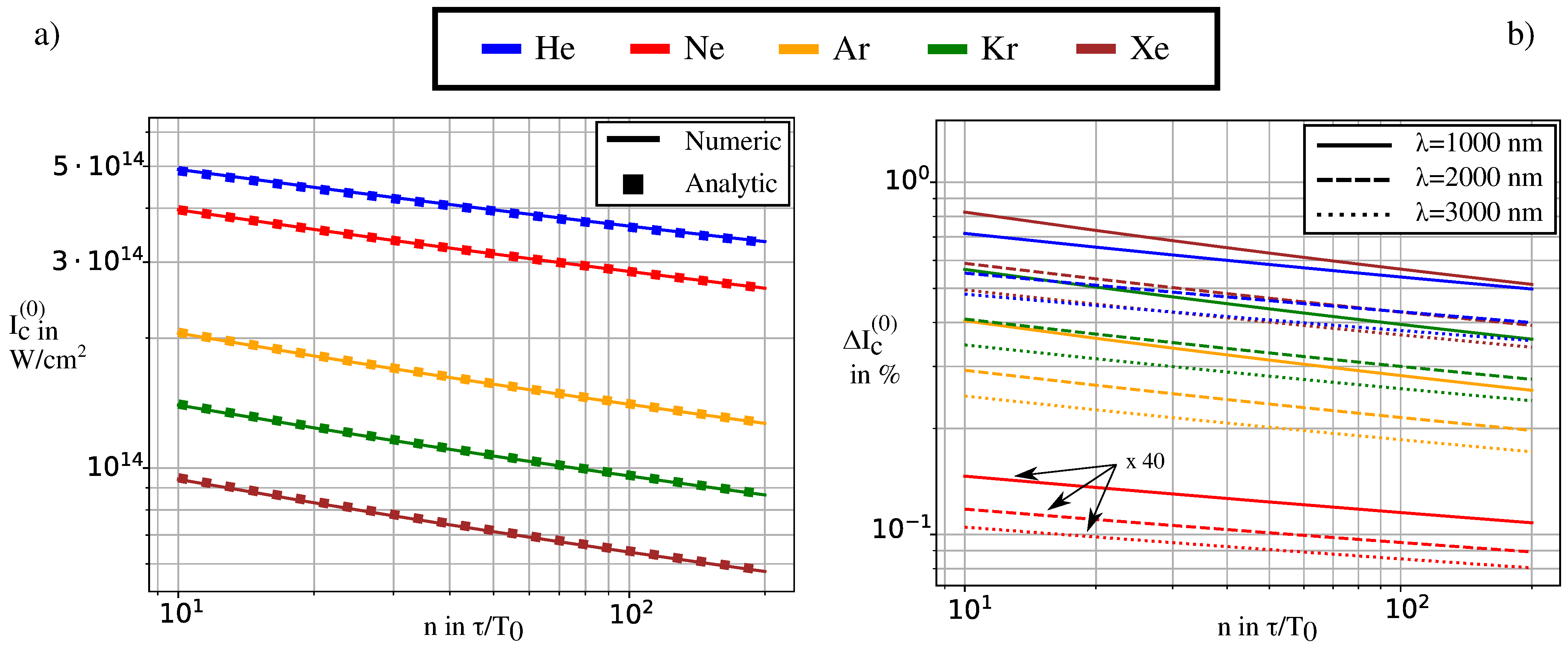
3.1. Accuracy Critical Intensity: Tunnel Ionization (ADK)

We begin with a visual comparison of the critical intensity calculated analytically and numerically. The critical intensity in Figure 2a is shown about the number of optical periods n, which is proportional to the pulse duration n = τ / T 0 . Moreover, the wavelength of the incident laser pulse is fixed as λ = 1000 nm and the atomic species is denoted by the line color. The analytical results of Equation (11) are denoted by squares and the numerical results are as a solid line.
Because the difference between the numerical and analytical results is hardly visible, we display the error (40) of the critical intensity I c ( 0 ) for a set of wavelengths λ = 1000 , 2000 , 3000 nm (line type) and noble gases (line color) in Figure 2b. It is quite remarkable that the error is below 1 % for all parameter configurations, especially if we consider the number of approximations and assumptions we made in our derivation.
The error is not significantly sensitive to the harmonic energy; thus, this error estimate is valid for HH photon energies in the range from 25 eV to 200 eV . The upper limit of our calculations is arbitrarily set to 200 eV , which can be seen in Figure 1b. Nevertheless, the critical ionization probability remains fairly constant for the laser pulse parameters discussed in this paper such that the upper limit can be easily extended to photon energies of 2 keV .
One can see that the error of the critical intensity decreases with an increasing wavelength of the incident laser pulse as well as exponentially decreases with an increasing pulse duration. In addition, note that the error decreases with increasing ionization potential for all noble gases, except for helium. Because helium in the ground state does not have electrons in the p-orbital, the contributions of ionized electrons from bound states with m = ± 1 do not contribute to the numerical calculations compared to the other noble gases.
The accuracy of Equation (11) compared to a numerical computation can be seen for various configurations in Table 2. Here, we show the shortest wavelength λ min and the smallest number of optical periods n min for which the error is smaller than Δ I c ( 0 ) . This holds for n > n min and λ > λ min , as the error decreases for increasing n and λ . As a brief conclusion, the error of Equation (11) obeys
τ 20 fs , λ 800 nm , n 8 Δ I c ( 0 ) 1.0 % ,
and holds true for all noble gases. To compare the computation times, we fix the parameters λ = 1000 nm , I p = 15.76 eV (Ar: = 1 ), and η c = 0.02 for a high-harmonic photon energy of E q > 100 eV . We compare the critical intensity for pulse duration of n = 20 τ / T 0 and n = 100 τ / T 0 . The numerical computation is executed in the Julia programming language [29] and uses the QuadGK package [30] for numerical integration and the NLsolve package [31] for the root-finding algorithm. The resulting computation times are denoted as t A ( n ) and t N ( n ) for the analytical and numerical computation, respectively. The average computation times for n = 20 τ / T 0 are t A ( 20 ) = 736 ns compared to t N ( 20 ) = 830 · 10 5 ns ; thus, the analytical method is roughly 10 5 times faster. For the pulse duration n = 100 τ / T 0 , the analytical method is roughly 10 6 times faster with t A ( 100 ) = 725 ns compared to t N ( 100 ) = 447 · 10 6 ns . Here, one can see the potential relevance for more advanced investigations that need to calculate the critical intensity many times. Overall, the ratio for the computation times of the critical intensities, calculated from the respective PPT model, is 10 4 to 10 5 . This ratio is approximately one order of magnitude lower than the ratio for the critical intensity in the ADK model, which may be explained by the iterative application of the critical intensity Equation (37).
For wavelengths shorter than 800 nm , the ADK model is no longer valid. We proceed further with the critical intensity calculated within the PPT model.

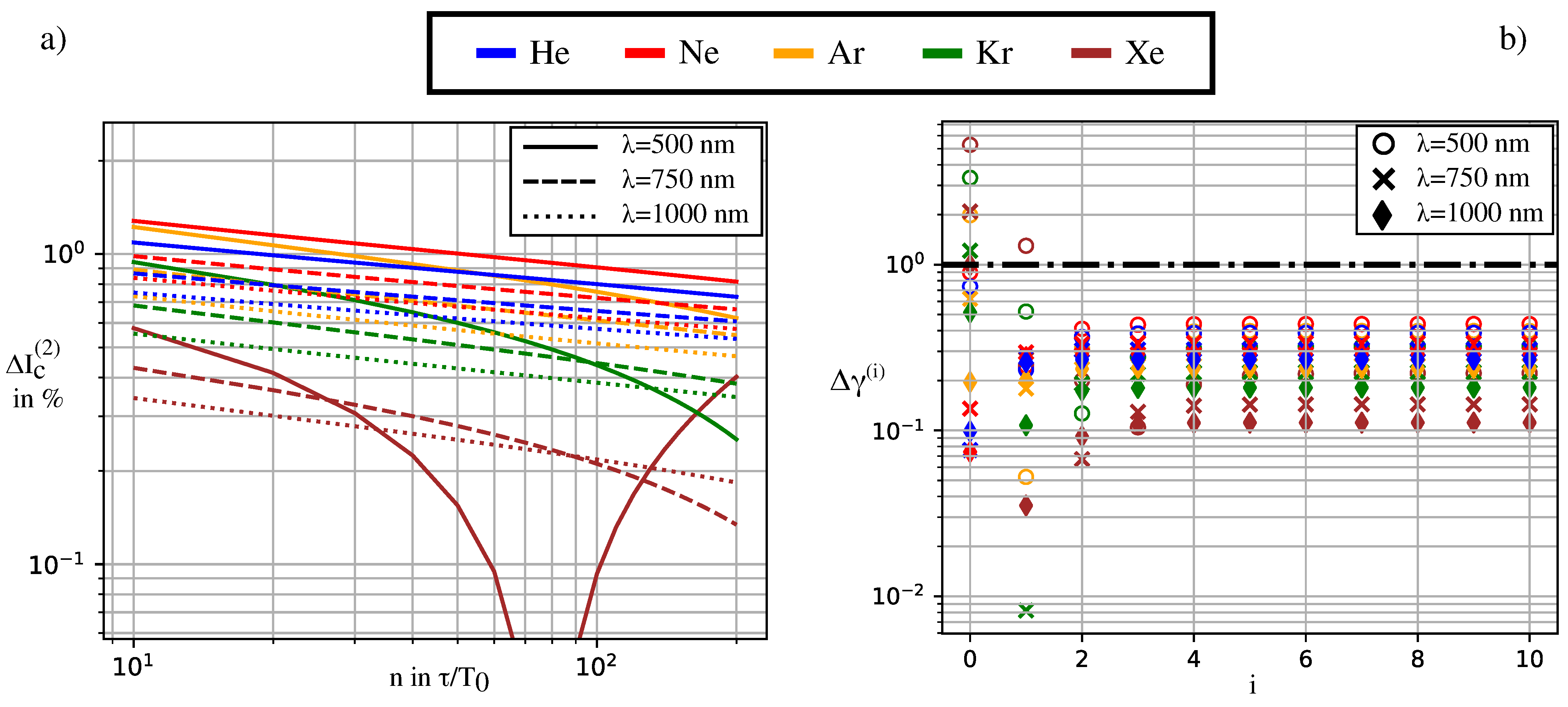
3.2. Accuracy Critical Intensity: Tunnel and Multi-Photon Ionization (PPT)

Going on to shorter wavelengths of the laser pulse leads us to the regime in which tunnel and multi-photon ionization need to be considered simultaneously. In this regime, the Keldysh parameter is on the order of one such that we need to calculate the critical intensities with the PPT ionization model. We use Equation (37), where i increases with increasing Keldysh parameter until the Keldysh parameter converges.
In Figure 3a, one can see the error of the critical intensity (37) for i = 2 , similar to Figure 2b. In contrast to Figure 2b, the error of heavy noble gases such as krypton and xenon deviates from the exponential decrease with increasing pulse duration. In addition, the error gets fairly large for long pulse durations. This unusual scaling of the error in krypton and xenon is related to the number of iteration steps i in (37). Because the critical Keldysh parameter γ c ( i ) is larger for small ionization potentials, as in the case of krypton and xenon, the number of iterations needs to be larger as well. Figure 3b shows the convergence of the Keldysh parameter with iteration step i on the x-axis and the error of the Keldysh parameter on the y-axis. Here, we fixed the pulse duration to τ = 200 T 0 . The iteration step i = 0 calculates the Keldysh parameter by using the critical intensity of the ADK model. The Keldysh parameter converges for increasing iteration steps i and wavelengths of λ = 500 , 750 , 1000 nm (marker type) fairly quickly to an error of less than 1 % .
Similar to the critical intensity in the ADK model, the error is not significantly sensitive to the energy of the HH photon, hence we can neglect it. The accuracy of the critical intensity in the PPT model is shown for various configurations in Table 3. Overall the accuracy of (37) obeys
τ 8.3 fs , λ 250 nm , n 10 Δ I c ( i ) 2.5 % ,
τ 8.6 fs , λ 515 nm , n 5 Δ I c ( i ) 1.5 % ,
τ 26.7 fs , λ 800 nm , n 10 Δ I c ( i ) 1.0 % ,
for all noble gases. Here, the computation time of the numerical integration is also 3 to 4 orders of magnitude higher than for our analytical approach (37). Note, the iteration step parameter i is chosen such that the critical intensity is converged and is therefore not fixed.

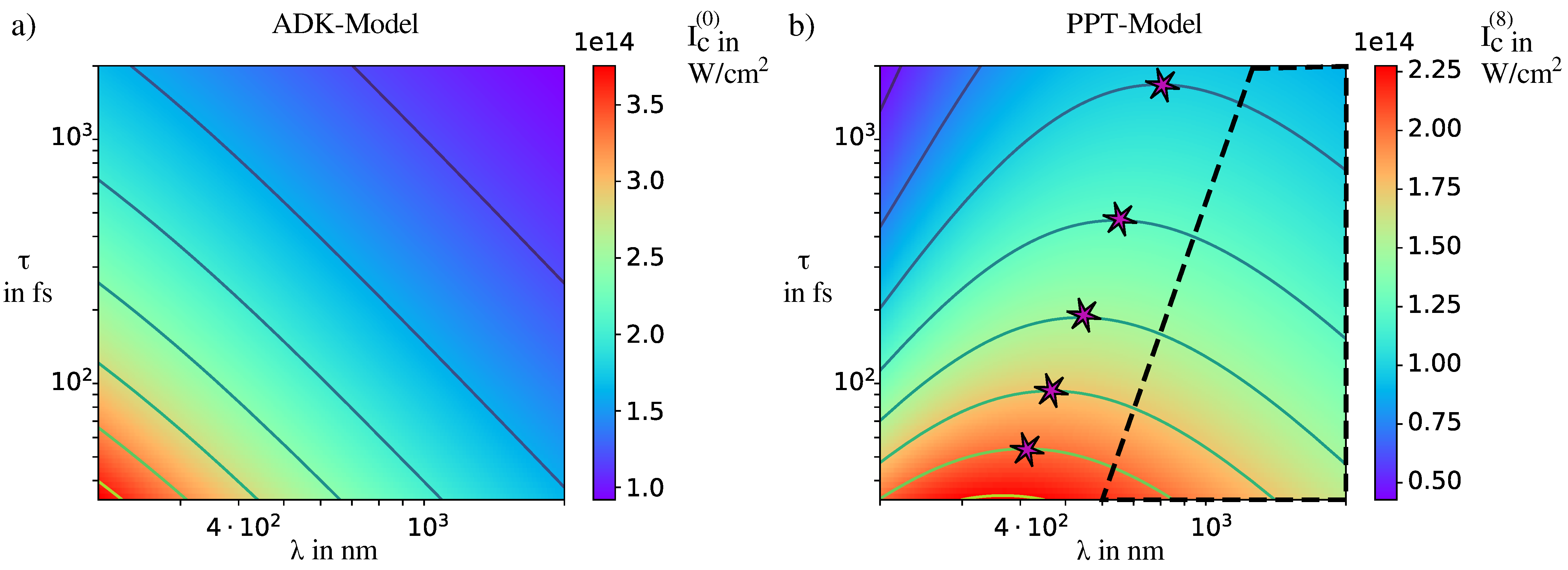
3.3. Critical Intensity: Comparison ADK—PPT

As we have already discussed the accuracy of the critical intensities (11) and (37), in this section, we focus on the interpretation of their respective results. In particular, we focus on the general scaling of the critical intensity concerning the pulse duration and the incident wavelength. Figure 4 shows two density plots of the critical intensity I c ( i ) ( λ , τ ) (color scale) in which the variation of the wavelength is located on the horizontal axis and the variation of the pulse duration on the vertical axis. Figure 4a,b show the critical intensity of the ADK and the PPT model in argon, respectively. Specifically, the critical intensity within the ADK model increases constantly with shrinking wavelength and pulse duration. This is highlighted by the contour lines (solid) that denote parameter compositions ( λ , τ ) with constant critical intensity. These lines represent the solutions of Equation (16) inserted into I c ( i ) ( λ , τ ) . The pulse duration scaling matches well with our analytic approximation in Equation (17), whereas the wavelength scaling is related to the critical ionization probability that does not show a closed form of its scaling. As noted before, Figure 4b shows the critical intensity in the PPT model. First, let us focus on the dashed inset on the right side. Here, the scaling of the critical intensity matches well with the ADK model such that the respective structure of the contour lines agrees. However, outside of the inset, the scaling changes drastically. The deviation is remarkable, as the global scaling changes rapidly. The change in the global scaling is visualized by the purple stars to the left of the dashed inset. The position of these stars can be interpreted as follows.
If we select an arbitrary pair of parameters ( λ 0 , τ 0 ) inside the dashed inset, then we can constantly decrease the wavelength while keeping the pulse duration constant, which leads to a monotonic increase in the critical intensity. At a specific wavelength, the critical intensity will not increase anymore but remains constant and will decrease afterward. The purple star denotes the wavelength λ 0 at which the intensity remains constant such that it describes the transition between two separated regimes. In the first regime, the critical intensity increases for decreasing wavelength; in the second, the critical intensity decreases with decreasing wavelength. Even though the number of purple stars that are shown in Figure 4b is finite, in general, they represent an infinite collection of points.
From a more pragmatic point of view, the purple stars denote the highest critical intensity that can be applied to generate phase-matched high-order harmonics, for a given pulse duration τ .
As noted above, the data shown in Figure 4b was computed by the analytical formula of the critical intensity in the PPT model Equation (37). The computation time for this 1000 × 1000 data grid (wavelength and the pulse duration) is, on average, 97 s . A numerical algorithm as defined below Equation (10) would need the same computation, approximately 97 s · 10 4 = 270 h , or 11 days.

4. Conclusions

In this work, we demonstrated an approach to calculate the critical intensity of phase-matched high-order harmonic generation analytically. The derived formulas are valid in the tunnel ionization regime (ADK-model) and get extended to the intermediate regime of tunnel and multi-photon ionization (PPT model). The analytic formulas for the critical intensity in both ionization regimes are highly accurate and can replace numerical computations while benefiting from a decrease in the computation time of approximately 4 to 6 orders of magnitude. We analyzed the accuracy of the developed approximations for the commonly used parameter space of all noble gases and listed the errors for specific sub-spaces. In addition, we discussed the analytic scaling properties of the critical intensity with regard to the pulse duration and wavelength in the tunnel-ionization regime. Finally, we highlighted the differences between the critical intensities in the respective ionization regimes and displayed the suppression of this intensity in the intermediate ionization regime.
Overall, we demonstrated that the developed formulas of the critical intensity are highly accurate and show a significantly decreased computation time compared to a numerical solution.

Author Contributions

Conceptualization, B.M. and R.K.; Formal analysis, B.M.; Funding acquisition, S.F.; Investigation, B.M.; Methodology, B.M.; Project administration, B.M.; Software, B.M.; Supervision, S.F.; Validation, B.M.; Visualization, B.M.; Writing—original draft, B.M.; Writing—review and editing, B.M., R.K., J.R. and S.F. All authors have read and agreed to the published version of the manuscript.

Funding

This work has been funded by the Deutsche Forschungsgemeinschaft (DFG, German Research Foundation) under project number 440556973, by the Fraunhofer Cluster of Excellence Advanced Photon Sources (CAPS), by the Innovation Pool of the Research Field Matter of the Helmholtz Association of German Research Centers in the project (ECRAPS), by APPA R&D: Licht-Materie Wechselwirkung mit hochgeladenen Ionen (13 N12082), by the Thüringer Ministerium für Bildung, Wissenschaft und Kultur (501100004404, 2017 FGR 0076), by the Thüringer Aufbaubank (TAB Forschergruppe 2015FGR0094), and by the Helmholtz association under grant agreement HGF ExNet-0019-Phase 2–3.

Conflicts of Interest

The authors declare no conflict of interest.

References

  1. Klas, R.; Kirsche, A.; Gebhardt, M.; Buldt, J.; Stark, H.; Hädrich, S.; Rothhardt, J.; Limpert, J. Ultra-short-pulse high-average-power megahertz-repetition-rate coherent extreme-ultraviolet light source. PhotoniX 2021, 2, 4. [Google Scholar] [CrossRef]
  2. Popmintchev, D.; Galloway, B.R.; Chen, M.C.; Dollar, F.; Mancuso, C.A.; Hankla, A.; Miaja-Avila, L.; O’Neil, G.; Shaw, J.M.; Fan, G.; et al. Near-and extended-edge X-ray-absorption fine-structure spectroscopy using ultrafast coherent high-order harmonic supercontinua. Phys. Rev. Lett. 2018, 120, 093002. [Google Scholar] [CrossRef] [PubMed] [Green Version]
  3. Minneker, B.; Böning, B.; Fritzsche, S. Generalized nondipole strong-field approximation of high-order harmonic generation. Phys. Rev. A 2022, 106, 053109. [Google Scholar] [CrossRef]
  4. Chen, M.C.; Mancuso, C.; Hernández-García, C.; Dollar, F.; Galloway, B.; Popmintchev, D.; Huang, P.C.; Walker, B.; Plaja, L.; Jaroń-Becker, A.A.; et al. Generation of bright isolated attosecond soft X-ray pulses driven by multicycle midinfrared lasers. Proc. Natl. Acad. Sci. USA 2014, 111, E2361–E2367. [Google Scholar] [CrossRef] [PubMed] [Green Version]
  5. Popmintchev, T.; Chen, M.C.; Popmintchev, D.; Arpin, P.; Brown, S.; Ališauskas, S.; Andriukaitis, G.; Balčiunas, T.; Mücke, O.D.; Pugzlys, A.; et al. Bright coherent ultrahigh harmonics in the keV X-ray regime from mid-infrared femtosecond lasers. Science 2012, 336, 1287–1291. [Google Scholar] [CrossRef]
  6. Lewenstein, M.; Balcou, P.; Ivanov, M.Y.; L’huillier, A.; Corkum, P.B. Theory of high-harmonic generation by low-frequency laser fields. Phys. Rev. A 1994, 49, 2117. [Google Scholar] [CrossRef]
  7. Shiner, A.; Trallero-Herrero, C.; Kajumba, N.; Bandulet, H.C.; Comtois, D.; Légaré, F.; Giguère, M.; Kieffer, J.; Corkum, P.; Villeneuve, D. Wavelength scaling of high harmonic generation efficiency. Phys. Rev. Lett. 2009, 103, 073902. [Google Scholar] [CrossRef]
  8. Falcao-Filho, E.L.; Gkortsas, V.M.; Gordon, A.; Kärtner, F.X. Analytic scaling analysis of high harmonic generation conversion efficiency. Opt. Express 2009, 17, 11217–11229. [Google Scholar] [CrossRef]
  9. Gkortsas, V.M.; Bhardwaj, S.; Falcao-Filho, E.L.; Hong, K.H.; Gordon, A.; Kärtner, F.X. Scaling of high harmonic generation conversion efficiency. J. Phys. At. Mol. Opt. Phys. 2011, 44, 045601. [Google Scholar] [CrossRef]
  10. Weissenbilder, R.; Carlström, S.; Rego, L.; Guo, C.; Heyl, C.; Smorenburg, P.; Constant, E.; Arnold, C.; L’Huillier, A. How to optimize high-order harmonic generation in gases. Nat. Rev. Phys. 2022, 4, 713–722. [Google Scholar] [CrossRef]
  11. Constant, E.; Garzella, D.; Breger, P.; Mével, E.; Dorrer, C.; Le Blanc, C.; Salin, F.; Agostini, P. Optimizing High Harmonic Generation in Absorbing Gases: Model and Experiment. Phys. Rev. Lett. 1999, 82, 1668–1671. [Google Scholar] [CrossRef]
  12. Balcou, P.; L’Huillier, A. Phase-matching effects in strong-field harmonic generation. Phys. Rev. A 1993, 47, 1447–1459. [Google Scholar] [CrossRef]
  13. Altucci, C.; Starczewski, T.; Mevel, E.; Wahlström, C.G.; Carré, B.; L’Huillier, A. Influence of atomic density in high-order harmonic generation. JOSA B 1996, 13, 148–156. [Google Scholar] [CrossRef] [Green Version]
  14. Popmintchev, T.; Chen, M.C.; Arpin, P.; Murnane, M.M.; Kapteyn, H.C. The attosecond nonlinear optics of bright coherent X-ray generation. Nat. Photonics 2010, 4, 822–832. [Google Scholar] [CrossRef]
  15. Rothhardt, J.; Krebs, M.; Hädrich, S.; Demmler, S.; Limpert, J.; Tünnermann, A. Absorption-limited and phase-matched high harmonic generation in the tight focusing regime. New J. Phys. 2014, 16, 033022. [Google Scholar] [CrossRef] [Green Version]
  16. Paufler, W.; Böning, B.; Fritzsche, S. Coherence control in high-order harmonic generation with Laguerre-Gaussian beams. Phys. Rev. A 2019, 100, 013422. [Google Scholar] [CrossRef]
  17. Minneker, B.; Böning, B.; Weber, A.; Fritzsche, S. Torus-knot angular momentum in twisted attosecond pulses from high-order harmonic generation. Phys. Rev. A 2021, 104, 053116. [Google Scholar] [CrossRef]
  18. Balcou, P.; Salieres, P.; L’Huillier, A.; Lewenstein, M. Generalized phase-matching conditions for high harmonics: The role of field-gradient forces. Phys. Rev. A 1997, 55, 3204. [Google Scholar] [CrossRef]
  19. Klas, R. Efficiency Scaling of High Harmonic Generation Using Ultrashort Fiber Lasers. Ph.D. Thesis, Friedrich Schiller University Jena, Jena, Germany, 2021. [Google Scholar]
  20. Chang, Z. Fundamentals of Attosecond Optics; CRC Press: Boca Raton, FL, USA, 2016. [Google Scholar]
  21. Salières, P.; L’Huillier, A.; Lewenstein, M. Coherence Control of High-Order Harmonics. Phys. Rev. Lett. 1995, 74, 3776–3779. [Google Scholar] [CrossRef] [Green Version]
  22. Dalgarno, A.; Kingston, A. The refractive indices and Verdet constants of the inert gases. Proc. R. Soc. Lond. 1960, 259, 424–431. [Google Scholar]
  23. Born, M.; Wolf, E. Principles of Optics: Electromagnetic Theory of Propagation, Interference and Diffraction of Light; Elsevier: Amsterdam, The Netherlands, 2013. [Google Scholar]
  24. Chantler, C.; Olsen, K.; Dragoset, R.; Chang, J.; Kishore, A.; Kotochigova, S.; Zucker, D. X-ray Form Factor, Attenuation and Scattering Tables (Version 2.1); National Institute of Standards and Technology: Gaithersburg, MD, USA. Available online: http://physics.nist.gov/ffast (accessed on 20 June 2022).
  25. Yudin, G.L.; Ivanov, M.Y. Nonadiabatic tunnel ionization: Looking inside a laser cycle. Phys. Rev. A 2001, 64, 013409. [Google Scholar] [CrossRef]
  26. Ammosov, M.V.; Delone, N.B.; Krainov, V.P. Tunnel ionization of complex atoms and of atomic ions in an alternating electromagnetic field. Sov. J. Exp. Theor. Phys. 1986, 64, 1191. [Google Scholar]
  27. Veberic, D. Having fun with Lambert W (x) function. arXiv 2010, arXiv:1003.1628. [Google Scholar]
  28. Perelomov, A.; Popov, V.; Terent’Ev, M. Ionization of atoms in an alternating electric field. Sov. Phys. JETP 1966, 23, 924–934. [Google Scholar]
  29. Bezanson, J.; Edelman, A.; Karpinski, S.; Shah, V.B. Julia: A fresh approach to numerical computing. SIAM Rev. 2017, 59, 65–98. [Google Scholar] [CrossRef] [Green Version]
  30. Johnson, S.G. QuadGK.jl: Gauss–Kronrod Integration in Julia. 2013. Available online: https://github.com/JuliaMath/QuadGK.jl (accessed on 20 June 2022).
  31. Mogensen, P.K.; Riseth, A.N. Optim: A mathematical optimization package for Julia. J. Open Source Softw. 2018, 3. [Google Scholar] [CrossRef]
Figure 1. (a) HHG-setup: laser pulse (orange-red), atomic targets (gray), generating medium (green), high-order harmonic radiation (blue), gas-jet emitter (gray-black); and (b) critical ionization probability η c (log scale) of commonly used noble gases with regard to the photon energy of the emitted harmonics E q at the fundamental laser wavelength of λ = 1000 nm .
Photonics 10 00024 g001
Figure 2. (a) The critical intensity (log scale) is calculated as a function of the pulse duration measured in multiples of the optical period (log scale). The ionization rates are calculated within the ADK model for a wavelength of λ = 1000 nm in neutrally charged noble gases (color). (b) Error of the analytic solution compared to the numerical integration (log scale) depending on the pulse duration (log scale) for wavelengths of λ = 1000 , 2000 , 3000 nm (line type) in neutrally charged noble gases (line color).
Photonics 10 00024 g002
Figure 3. (a) The error of the critical intensity (log scale) as a function of the pulse duration (log scale) was calculated within the PPT model. The error is shown for wavelengths of λ = 500 , 750 , 1000 nm (line type) in neutrally charged noble gases (line color). (b) Error of the Keldysh parameter (log scale) for a pulse of n = 200 optical periods (FWHM) about the number of iterations i. The set of wavelengths (marker style) and noble gases (line color) is the same as in a).
Photonics 10 00024 g003
Figure 4. Density plots of the critical intensity in argon calculated within the ADK model (a), and the PPT model for iteration step i = 8 (b). The critical intensity is shown for an incident wavelength from λ = 200 nm to 2000 nm (log scale) and a pulse duration of τ = 40 fs up to τ = 2000 fs (log scale). The inset in (b) denotes the parameter space for which the critical intensity calculated within the PPT model scales similarly (approximately linear contour lines) to the critical intensity calculated by the ADK model (a).
Photonics 10 00024 g004
Table 1. List of atom-dependent parameters to calculate the critical intensity in Equations (11) and (12).
HeNeArKrXe
g 0 −0.5122−0.4114−0.1417−0.02830.1182
F 0 1.61961.33030.83110.69580.5612
κ 0 6.57146.42046.12006.02265.9116
Table 2. Accuracy of the critical intensity in the ADK model (40). The table is showing the lower limit of the parameters λ min , n min , τ min λ min n min (wavelength, number of optical cycles, pulse duration) for which the error of the critical intensity is smaller than Δ I c ( 0 ) . The error decreases for any configuration of higher parameters. We fixed the HH photon energy to 50 eV such that the error of the critical intensity remains roughly constant for higher photon energies and changes reasonably slowly for lower photon energies, such as the critical ionization probability in Figure 1b.
Element λ min in nm n min τ min in fs Δ I c ( 0 )
He800718.7 1.0 %
16001053.4 0.7 %
3200553.4 0.6 %
Ne80038.0 < 0.01 %
1600316.0 < 0.01 %
3200332.0 < 0.01 %
Ar80038.0 < 0.5 %
1600316.0 < 0.4 %
3200332.0 < 0.3 %
Kr800410.7 < 0.7 %
1600421.4 < 0.5 %
3200442.7 < 0.4 %
Xe800513.3 1.0 %
1600526.7 0.7 %
3200553.4 0.5 %
Table 3. Accuracy of the critical intensity in the PPT model (41). The table is showing the lower limit of the parameters with the respective wavelength λ min , number of optical cycles n min , and the resulting pulse duration τ min λ min n min for which the error of the critical intensity is smaller than Δ I c ( 0 ) . The iteration parameter i is not fixed and is chosen such that the critical intensity is converged. We fixed the HH photon energy to 50 eV such that the critical intensity remains roughly constant for higher photon energies and, thus, the change in the error for lower photon energies is reasonably small.
Element λ min in nm n min τ in fs Δ I c ( i )
He25054.2 2.5 %
51558.6 < 1.5 %
8001026.7 1.0 %
Ne25097.5 2.5 %
51558.6 1.5 %
800821.4 1.0 %
Ar250108.3 2.5 %
51535.2 1.5 %
800410.7 1.0 %
Kr25054.2 < 2.5 %
51535.2 < 1.5 %
80038.0 < 1.0 %
Xe25032.5 < 2.5 %
51535.2 < 1.0 %
80038.0 < 1.0 %
Disclaimer/Publisher’s Note: The statements, opinions and data contained in all publications are solely those of the individual author(s) and contributor(s) and not of MDPI and/or the editor(s). MDPI and/or the editor(s) disclaim responsibility for any injury to people or property resulting from any ideas, methods, instructions or products referred to in the content.

