Calculation of Black Ice Thickness and Heat Fluxes inside the Ice and at the Water–Ice Boundary in a Boreal Lake

Abstract

This paper presents the results of the calculation of black ice thickness, as well as conductive heat fluxes inside the ice and at the water–ice boundary during the winter in the shallow boreal Lake Vendyurskoe (Russia). The calculation was carried out on the basis of experimental data obtained from a thermistor chain with nine sensors, five of which were successively frozen into the black ice during the winter of 1995–1996. Data processing was carried out by two methods, whose novelty lay in the simultaneous use of the temperature series of two sensors frozen into the ice and those that were in the water column directly under the lower ice boundary. The resulting estimates of black ice growth rates varied widely: maximum values (up to 8.5 mm/day) were observed in December during first month of ice period, with an average growth rate of 3.4 mm/day from December to the end of February. The heat flux in the black ice sheet varied significantly over synoptic time intervals; the highest values (up to 40 W/m²) were observed during the first two weeks of measurements, then a downward trend was noted, to values of ~10 W/m². Black ice was isothermal from the end of February to the end of April due to the release of water on the ice surface after heavy snowfall. During this period the heat flux inside the black ice was zero, and there was no increase in black ice thickness. The calculation of the water–ice heat flux gives results that are very sensitive to both measurement limitations and the variability of external parameters. However, the estimates of this flux for moments in time when the sensors were frozen in the ice are values 1–2 W/m², which are quite close to the previous estimates for Lake Vendyurskoe. The limitations of the presented method are related to the thermal inertia of black ice and make it possible to calculate of ice thickness with a time delay of several days. To quantify the effects of thermal inertia of ice, a model problem of heat propagation in the ice sheet is considered for the case of periodic temperature changes at its upper boundary. The attenuation of the amplitude and the delay of a heat wave during its propagation in the ice are estimated, and accordingly, the conditions, under which the temperature profile in the ice sheet is close to linear, are analyzed.

1. Introduction

In recent decades, against the background of climate change, there has been a shortening of ice-covered period on lakes of temperate zones and high latitudes [1,2]. Along with changes in ice phenology, ice thickness decreases, and its composition changes due to an increase in the proportion of white ice [3,4]. These factors affect the thermal, hydrodynamic, light and gas regimes of lakes, and chemical and biological processes, which makes it important to study changes in the ice regime of lakes under current climatic conditions [5,6]. In this regard, the study of the physical mechanisms responsible for the formation, growth, and melting of ice in lakes becomes an urgent task [7,8]. In turn, the parameterization of heat and mass transfer processes in the ice and at its boundaries with air and water play a special role [9,10,11,12,13,14,15,16].

The ice cover of temperate lakes usually includes two main layers—black and white (snowy) ice [7,8,10,16]. Black ice is formed from water. Its growth rate decreases after snowfall, as snow effectively insulates the ice from thermal interaction with the atmosphere. An increase in the thickness of black ice occurs due to the ice buildup at the boundary with water, provided that the ascending conductive heat flux in the ice exceeds the heat flux from water to its lower boundary. The growth and melting rates of black ice depend on many factors, including air and water temperature, water stratification, currents, turbulence intensity in the water layer adjacent to the ice, and solar radiation fluxes [8,17,18]. Sometimes in winter there is a layer of water on the ice surface. There are several reasons for the appearance of water on ice: rain or wet snow falls at positive air temperatures, melting of snow and ice during thaws, and release of lake water to the ice surface through cracks in the ice [15,19,20]. When there is water layer on the ice surface, the temperature at the upper and lower boundaries of ice is close to the freezing point, while the temperature inside the ice is also close to 0 °C, causing the ice to become isothermal [19]. In such conditions the thickness of the black ice does not increase.

White ice forms after heavy snowfalls when water escapes onto the surface of black ice through cracks and the water-soaked snow freezes, or when wet snow falls and then freezes [8,9,10,16,19,20]. The change in the thickness of white ice is mainly influenced by precipitation, the frequency of alternating periods of thawing and cooling, solar radiation fluxes, and air temperature.

To calculate the thickness of black ice, it is necessary to estimate the heat fluxes at its boundaries with air/snow/white ice and water, and the heat flux through the ice sheet. It is also necessary to take into account the turbulence of the under-ice water layer [17,18] and white ice and/or wet snow (slush). All these factors can introduce a large uncertainty into the calculations, which necessitates their in-depth study.

Methods for calculating the thickness of black ice, and heat fluxes inside the ice sheet and at the boundary of ice with water, based on both sounding data and autonomous measurements, are constantly being improved.

Conductive heat flux q_ice through ice can be estimated using the one-dimensional Fourier thermal equation q_ice = −λ_ice ∂T/∂z, where ∂T/∂z is the temperature gradient in the ice (°C/m), and λ_ice is the thermal conductivity of ice [21]. However, it should be borne in mind that the vertical temperature profiles in ice changes both during the day and on the synoptic time scale due to air temperature changes and precipitation. Due to the decrease in the amplitude of diurnal temperature fluctuations in the ice sheet with depth, as well as their phase delay, a non-monotonic vertical temperature distribution is formed in ice sheets [19,21]. Accordingly, the calculation of the temperature profile within the ice and the assessment of the temperature gradient directly at the interface of ice with water in the general case is a difficult task [22].

Estimations of heat flux q_w from water to ice also remain challenging. Here, one of the methods is based on using the growth rate of black ice and the value of the vertical temperature gradient measured in the ice [16,21]. Assuming that the temperature in the ice changes in proportion to the distance from the boundary (linearly), the heat flux q_w can be estimated from the heat balance equation at the lower ice boundary [16] by using Stefan’s relation (see Formula (2) below).

In the framework of the so-called bulk method, the heat flux from water to ice is calculated using the following formula (hereinafter, the index w is used to designate water parameters): q_w = ρ_wc_wC_H(T − T₀)U_w, where ρ_w is the density of water, c_w is the specific heat of water, C_H is the heat transfer coefficient, T is the water temperature under the ice, T₀ is the temperature at the bottom of the ice, and U_w is the water flow velocity [10,23].

One of the ways to estimate the heat flux from water to ice is to consider a laminar layer of water adjacent to the lower boundary of the ice. In this thin layer, heat transfer occurs at the molecular level, and the gradient method based on water temperature measurements is applicable [24,25]. However, the thickness of this laminar water layer is very small and amounts to several mm/cm, which requires measurements with high vertical resolution. Such measurements are possible when sounding the sub-ice water layer with highly sensitive instruments [26,27]. One of the disadvantages of this method is the discreteness of the obtained estimates over time: separate measurements during the winter season do not allow for the estimation of the small-scale variability of the heat flux at the water–ice boundary, depending on synoptic and other conditions [18,21,25]. In addition, sounding is carried out only in the water column, while the temperature of the black ice remains unknown.

These difficulties can be overcome by using autonomous systems that allow for long-term high-frequency (minutes) temperature measurements inside a multi component water–ice–snow–air system. Usually these complexes also provide measurements of other parameters (meteorological indicators, solar radiation fluxes in the ice sheet and under the ice, changes in the position of the ice surface, currents, etc.) that are necessary for the model calculation of the seasonal ice evolution, including its thickness. The list of such measuring systems includes SIMBA (Snow and Ice Mass Balance Array) [21,28,29,30], ASLIM (The autonomous system for lake ice monitoring) [22], and FROS (a floating remote observation system) [31]. Other variants of such systems are also known [16,25,32,33]. In such experimental complexes, temperature measurement in the water–ice–snow–air system is carried out on the same vertical with a discreteness of the location of temperature sensors of 2–10 cm [15,21,22,30]. Such discreteness (~ cm) is noticeably larger than in sounding (mm), which imposes restrictions on the applicability of the gradient method and reduces the quality of estimates of heat flux at the ice–water boundary.

Processing temperature measurement data in a multiphase environment is also a challenge. In particular, special algorithms are being developed to determine the boundaries of ice–water, ice–snow, and snow–air based on the records of autonomous temperature sensors [21,30]. Then, the ice and snow thicknesses are estimated as the distance between the detected boundaries. The average ice growth rates are calculated as the difference between the maximum recorded ice thicknesses in the selected time intervals.

As was stressed above, accurate estimates of ice thickness and heat fluxes require high-precision measurements of a large number of parameters and, accordingly, the use of complex multifunctional measuring systems. One of the most important elements of such complexes is temperature chains with a large number of sensitive sensors. A special role is played by chains, in which the sensors are located at a small distance from each other and are sequentially frozen into the ice during the experiment. This paper presents the results of an experiment in which a chain with temperature sensors was used autonomously for long-term temperature measurements in the thickness of black ice and in the under-ice water layer. It is shown that the corresponding temperature series make it possible, albeit with some limitations, to make an accurate assessment of both the dynamics of black ice thickness ξ, and heat fluxes q_ice and q_w without involving additional data such as air temperature, solar radiation fluxes, currents, etc. The experiment was carried out on the small boreal Lake Vendyurskoe (northwestern Russia) during the winter season of 1995–1996.

The proposed new method for calculating black ice thickness ξ and the heat fluxes from water to ice and in black ice sheet has several limitations. One of them is related to the need to take into account the thermal inertia of ice. To quantify the effects of inertia, a model problem of heat propagation in the ice sheet is considered for the case of periodic temperature changes at its upper boundary. The amplitude attenuation and delay of a thermal wave during its propagation in the ice sheet are calculated.

2. Materials and Methods

2.1. Study Site

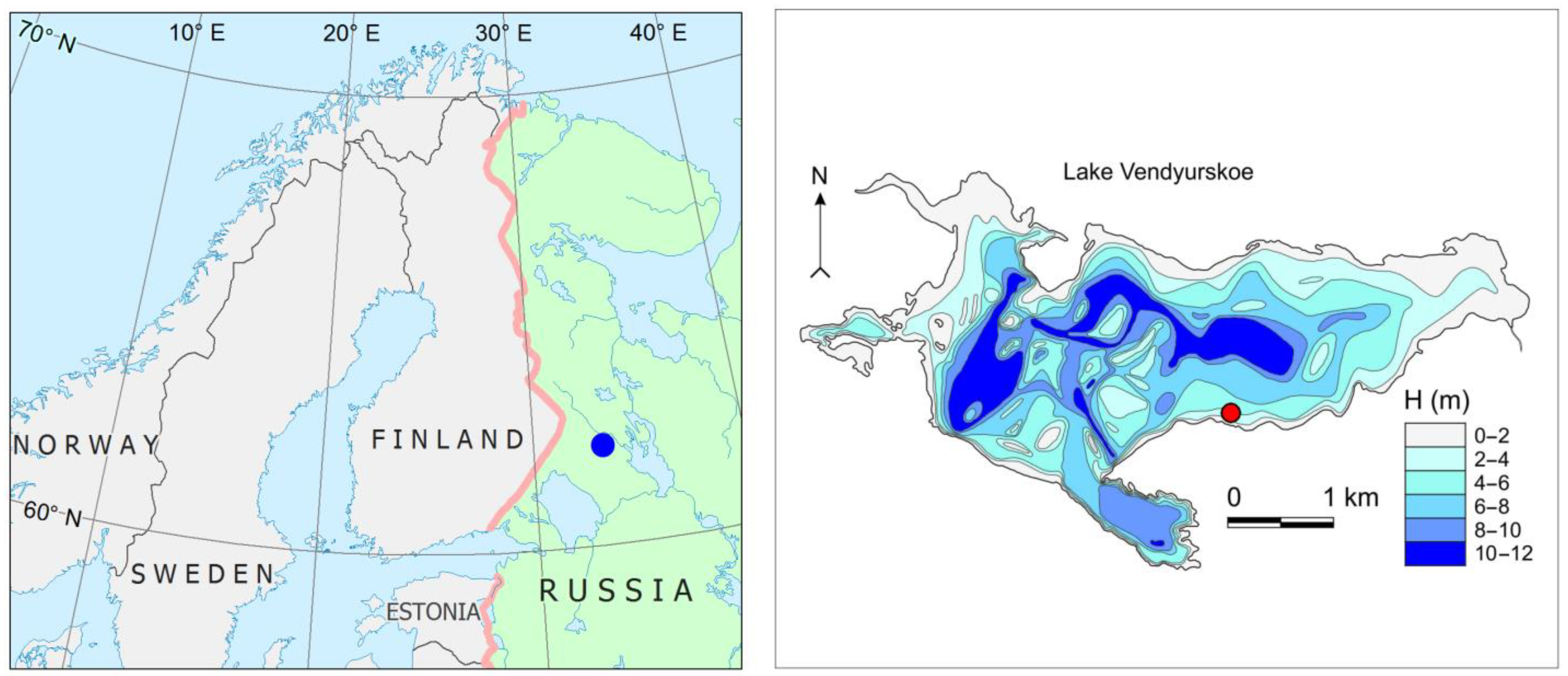
Measurements of water and ice temperature were carried out in the shallow boreal Lake Vendyurskoe during the winter season of 1995–1996. This is a small lake of glacial origin in northwestern Russia (62°13′ N, 33°16′ E) (Figure 1). The area of the lake is 10.2 km², the average and maximum depths reach 5.3 and 11.4 m. Ice formation on the lake occurs from the beginning of November to mid-December in different years, and ice breaking occurs from the end of April to the middle of May. During the winter of 1995–1996 ice cover lasted from 7 November 1995 to 14 May 1996.

Measurements of water and ice temperature were carried out using an autonomous chain developed at Northern water problems Institute of the Karelian Research Center of the Russian Academy of Sciences. Nine semiconductor microthermal resistors, MT-57 (made in Russia), were used. Sensors’ calibration was carried out at the Northern Water Problems Institute using a thermostat. Particular attention was paid to the temperature range near the freezing point of fresh water, which is 0 °C. For this purpose, additional calibration and intercalibration of the sensors was performed in a container filled with lake water with snow in the absence of light and an air humidity of about 100%. The resolution of the temperature sensors was 0.003 °C, and the accuracy was 0.05 °C.

The chain was installed on the ice on 1 December 1995 when the thickness of black ice reached 24 cm. The time interval of measurements was two hours. The temperature sensors were distributed with a vertical step of Δl = 0.10 m. When the chain was installed, two upper sensors were in the water in the hole at a distance of 0.12 and 0.22 m from the black ice surface, and other sensors were in the water under the lower boundary of ice. Two sensors in the hole were frozen into the ice within the first few hours of measurements. During the winter the next three sensors consistently froze into the ice. The chain was removed from the lake on 23 May 1996, a week after ice-off. The depth of measurement station was 4.4 m. Figure 2 shows a sketch of the position of the sensors in the black ice and in the subglacial water.

Measurements of the thickness of snow and ice in the hole drilled near the measurement station were carried out eight times during the winter season of 1995–1996: 25 November 1995 (before the installation of an autonomous chain), 1 and 25 December 1995; 20 March 1996; and 16, 19, 20, 21, 22 and 24 April 1996. To measure snow and ice thickness a hydrological L-shaped ruler was used, which was hooked onto the lower edge of the ice in the hole, and the reading was taken along the upper edge of the ice and snow. The accuracy of measuring the thickness of ice and snow was 0.5 cm. It was impossible to determine the thickness of black and white ice separately, since their boundary was below the water level in the hole.

The weather conditions during the winter of 1995–1996 were characterized using data from the Petrozavodsk weather station [34]. The analysis used data on air temperature and precipitation. This weather station is located 70 km from Lake Vendyurskoe to the southeast. The correlation of the air temperature series at the Petrozavodsk weather station and the air temperature measured near Lake Vendyurskoe in different seasons in different years was very high, and the correlation coefficient reached 0.98.

2.2. Analysis of Temperature Profile in the Ice Sheet

Two methods were used to calculation heat fluxes, as well as the thickness and growth rate of the black ice. Within the framework of the first method, the calculations were carried out on the basis of the analysis of the temperature series of those sensors, which, during the experiment, turned out to be frozen into the ice.

Since the distance of the sensors from the upper black ice boundary was known, a preliminary rough assessment of black ice thickness was carried out directly for the moments of the successive freezing of the sensors into the ice.

The sensitivity of temperature sensors turned out to be high enough to determine such moments almost unambiguously. Thus, in the early winter, at the stage of active black ice growth with a rate of ~5 mm/day and a temperature gradient in the ice sheet of 20 °C/m, the characteristic temperature difference between two successive measurements in 2 h was ~0.01 °C. The latter value is comparable to the resolution of the sensors, which in most cases made it possible to unambiguously register the moment closest in time to freezing the sensor into the ice. Such estimates make it possible to determine the thickness of black ice with great accuracy, but only for the three time moments during winter (moments of sensors freezing to black ice).

In order to reconstruct the evolution of black ice thickness with high discreteness in time, an analysis of temperature profiles in the ice sheet was carried out. Under stationary conditions, when the temperatures of the upper and lower ice boundaries are fixed, a linear temperature profile is established in the ice sheet. The vertical gradient can be estimated as Γ = ΔT/Δl, where ΔT is the temperature difference between any two adjacent frozen sensors. On the other hand, for any time t, one may estimate the gradient by taking into account the temperature T*(t) of the frozen-in sensor closest to the lower ice boundary with the temperature 0 °C. The distance l* of this sensor from the upper black ice boundary is known (Figure 2), so its distance from the water–ice boundary is (ξ(t) − l*), and the gradient can be represented as Γ = (0 − T*(t))/(ξ(t) − l*). Using both relations for Γ, the following explicit expression for ice thickness ξ is derived for any time t:

$$\xi \left(t\right)=l^{*}+∆l{T}^{*}\left(t\right)/∆T\left(t\right)$$

(1)

2.3. Effects of Nonstationarity

In a general case, however, the problem is non-stationary; the temperature of the upper surface of black ice in contact with air, wet or dry snow, or water varies significantly with time. Such non-stationarity can significantly complicate the analysis of both heat fluxes and the dynamics of the growth of black ice. Since, due to the thermal inertia of the black ice sheet, the change in temperature at different points of ice sheet does not occur synchronously, temperature perturbations at the upper ice boundary penetrate downward with some delay and with a decrease in amplitude [35]. Such features are usually associated with a heat wave. The vertical temperature profile in this case is not linear. Accordingly, the possibility of estimating the temperature gradient at the lower boundary of black ice using the simple relation ∆T/∆l, as in Formula (1), requires verification.

All the mentioned effects of non-stationarity (time delay, amplitude decay, profile nonlinearity) significantly depend on the thermal inertia of ice, more precisely, on the ratio α = τ₁/τ₂ of two time scales τ₁ and τ₂. The first specifies the characteristic relaxation time of the temperature profile in black ice with thickness ξ: τ₁~ξ²/k, where k is the molecular temperature conductivity of ice. The value of τ₂, in turn, characterizes the scale of temperature disturbances at the upper black ice boundary. For the case when these disturbances are harmonic in time, the delay and damping are calculated analytically, the results from which are given in Appendix A (Figure A1). As shown by these calculations, a significant decrease in the amplitude of heat flux oscillations at the lower ice boundary compared to the upper one occurs only at sufficiently large values of the parameter α; in the case when α ∈ (0,1) the amplitude decreases by no more than 17%. As for the delay, at α < 1 the phase shift is sufficient but does not exceed 1 radian. When α < 0.4, amplitude attenuation and delay are, respectively, 3% and 0.4 radians, so for this case, non-stationary external conditions do not lead to a significant distortion of the linearity of the temperature profile.

The case of small α can be called quasi-static; here, the time of adaptation of the temperature profile (it is restructuring due to changed temperature at the upper ice boundary) is rather short compared to the characteristic external time scale. Thus, if the condition α < 1 is satisfied, it can be expected that non-stationary external conditions do not lead to a significant distortion of the temperature profile linearity, and Formula (1) gives a correct but time-delayed estimate of the ice thickness.

At the same time, when calculating the rate of ice growth, the delay can lead to a significant error, which also increases with increasing ice thickness (the parameter α increases as ξ increases).

2.4. Analysis of Temperature Profiles in the Water Column. Heat Flux from Water to Ice

The analysis of the temperature series of the sensors that were located in the water near the ice–water boundary was carried out mainly in the context of estimates of the water–ice heat flux q_w. Such assessments are associated with significant difficulties. Thus, the direct calculation of the heat flux q_w using the formula q_w = − λ_w dT_w/dz and the value of the molecular thermal conductivity of water λ_w is possible only for a thin laminar layer. The thickness of this layer is very small, from several mm to several cm [18,26], even in comparison with the dimensions of the sensitive elements of the sensors, which significantly complicates the task of calculating q_w directly from experimental data.

An alternative method for calculating q_w is to use the Stefan condition at the lower ice boundary [25]:

$$L{\rho }_{ice}\frac{d\xi }{dt}={\lambda }_{ice}\frac{d{T}_{ice}}{dz}-{\lambda }_w\frac{d{T}_w}{dz},$$

(2)

where L = 333.5 kJ/kg is the specific heat of ice melting, and ρ_ice is the density of ice. The value of λ_ice changes in the range of (2.23, 2.32) as the temperature decreases from 0 °C to −30 °C.

Formula (2) makes it possible to calculate the flux q_w from the known values of the ice growth rate dξ/dt and the temperature gradient dT_ice/dz in the ice sheet. However, in a general case, there are problems with estimating the first of these quantities. Ice thickness ξ can be calculated by Formula (1), as described above, with a fairly high degree of accuracy, although with a time delay of several days. The acceptability of such a calculation is mainly due to the cumulative or integral over time and the character of the value of ξ:, which smooths out the delay effect. However, when calculating parameters local in time, such as the ice growth rate, this effect turns out to be much more critical and can lead to significant errors, which makes it difficult to use Formula (2) for the direct calculation of q_w.

At the same time, highly sensitive sensors make it possible to determine the dependence of temperature on time with high accuracy. Under certain conditions, the use of chains with frozen-in sensors makes it possible to transform the dependences T_w(t) of water temperature on time obtained in the experiment into the dependence T_w(z) of water temperature on the distance to the lower ice boundary [25], and, on this basis, to calculate q_w.

Indeed, the change of water temperature at the sensor closest to the ice located in the sub-ice water layer occurs due to its slow approach to the lower boundary of ice as black ice grows from below: in essence, such a sensor slowly scans the temperature of a thin sub-ice water layer. Under conditions of monotonous ice growth, such a scan makes it possible to determine the T_w(z) profile using the following formula:

$$\frac{d{T}_w}{dz}=\frac{d{T}_w}{dt}\frac{1}{d\xi /dt},$$

(3)

For a sensor approaching ice, the rate dT_w/dt of its temperature change immediately before freezing into ice can be determined with a sufficiently high degree of accuracy by interpolating the dependence T_w(t) at the time intervals immediately preceding freezing. Thus, Formula (3) can be considered as an additional relationship that links two parameters: dξ/dt and q_w (or dT_w/dz). On the whole, relations (2) and (3) represent a closed system of equations for finding the two specified unknowns. The limitation of this method, however, lies in the fact that the calculations of both quantities are possible only at time moments corresponding to the freezing of the sensors.

3. Results

3.1. Weather Conditions, Snow and Ice Thickness, and Temperature of Ice and Under-Ice Water during the Winter Season of 1995–1996

The air temperature in three winter months of 1995–1996 varied from −1.9 °C to −27.6 °C, averaging −10.9 °C (Figure 3a). At the time of chain installation, the thickness of the snow on the ice was 10 cm, and the thickness of black ice was 24 cm (Figure 3b). During December, January, and February, snow fell regularly, and by mid-March, the average snow layer over the lake area reached 30 cm (Figure 3b). On 26 February 1996, after a heavy snowfall and with a sharp increase in air temperature from −22.2 °C to −1.6 °C, a crack formed in the ice cover near the measurement station, and the water came out onto the surface of the black ice. The air temperature in March and in the first half of April varied from −15.2 °C to +7.6 °C, averaging −3.2 °C. Thus, against the background of not very frosty weather, the wet snow layer did not completely freeze, and the mixture of snow and water effectively isolated the black ice from atmospheric impact until mid-April. The temperature on all sensors in black ice corresponded to the ice freezing point (0 °C), i.e., black ice was isothermal during March and April (Figure 3c), and its thickness did not increase in this period. This is also evidenced by the fact that the sensor, located at a distance of 0.62 m from the surface of the black ice, remained in the subglacial water throughout the entire winter and never froze into the black ice (Figure 3c). That is, the thickness of black ice did not exceed 0.62 m throughout the winter. Measurements in the hole on 20 March 1996 showed that the total thickness of the ice had reached 71 cm (Figure 3b). Assuming that black ice grows only from below, this allows us to estimate the thickness of white ice was at least 9 cm and no more than 19 cm since the thickness of black ice at that moment was at least 52 cm (since the 0.52 cm sensor was in ice) and no more than 62 cm (since the 0.62 cm sensor was in water). The greatest total ice thickness was reached on 16 April 1996—79 cm—while the snow decreased noticeably to 7 cm. If we assume that the thickness of black ice did not change in March–April, then we can conclude that there was an increase in the thickness of white ice by another 8 cm during the period between successive measurements. Since the second half of April, against the background of sunny and warm weather, the ice began to melt. Over 8 days, from 16 April to 25 April 1996, the total thickness of the ice decreased by 7 cm, and the snow completely melted (Figure 3b).

In further analyses, we used only data obtained before the end of February, when temperature gradients were observed in the black ice sheet.

During two winter months, three sensors (located a distance of 0.32, 0.42, and 0.52 m from the upper boundary of black ice) were sequentially frozen into the black ice. The freezing of these sensors occurred, respectively, 11 and 24 December 1995, and 26 January 1996, i.e., after 10 days and 8 h, 23 days and 2 h, and 56 days and 18 h from the start of measurements. The set of temperature series for the five upper sensors of the chain is shown in Figure 4.

Each of the curves of a family of lines in Figure 4 illustrates a rather complex dependence of black ice temperature on time due to irregular fluctuations in external conditions (in particular, the temperature of air, snow, or water on ice). In this case, the possibility of calculating the dynamics of the thickness of black ice using Formula (1), as shown in the previous section, depends on the ratio α of the internal and external time scales. From early December to the end of February, the thickness ξ of black ice increased from 0.24 m to 0.50 m. Accordingly, the value of the time scale τ₁ increased monotonically in the range from 0.4 to 2.4 days.

At the same time, the characteristic (synoptic) period of external disturbances (air temperature) was about 3–7 days (Figure 3a). Thus, for the measurement period, the parameter α varied in the range of (0.1–0.8), which may indicate the quasi-static character of external disturbances and, accordingly, small deviations of the temperature profile from a linear dependence.

In order to directly verify this important provision, the calculation of the temperature difference ΔT between adjacent pairs of sensors in black ice was carried out (Figure 5). For all pairs, the temperature difference was almost the same throughout the experiment, except for the period of 19–29 December 1995. Considering that the sensors were fixed on the chain at the same (0.1 m) distance from each other, it can be concluded that the temperature profile in black ice was approximately linear for each time moment during the whole measurement period. As for the time interval of 19–29 December 1995, the variations of temperature difference between different pairs of sensors was due to a sensor failure at a depth of 0.12 m.

3.2. Thickness of Black Ice and Heat Fluxes within Ice

The assumption of linearity of the temperature profile in ice made it possible to directly calculate (see Formula (1)) the dynamics of the thickness ξ(t) of black ice, as well as the heat flux $q_{ice}=-{\lambda }_{ice}\frac{d{T}_{ice}}{dz}$. Here, the temperature gradient is determined directly from the temperature difference between adjacent sensors. The results of the calculations of the dynamics ξ(t) from 1 December 1995 to 15 March 1996 and heat fluxes from 13 December to 25 December 1995 are shown in Figure 6 and Figure 7, respectively. Figure 6 also schematically presents the results of an alternative (based on the solution of system (2) and (3)) calculation of the ice growth rate for the time points corresponding to the freezing of the sensors. The greatest thickness of black ice, according to the estimates obtained, does not exceed 0.55 m, which is consistent with the above estimates of its maximum thickness of no more than 0.62 m.

Based on the calculated values of q_ice and dξ/dt, the heat flux q_w from water to ice was also estimated by using the Stefan condition (2). The corresponding curve q_w(t), together with its smoothed (daily averaged) version ${\overline{q}}_w$, is also presented in Figure 7.

Independent estimates of black ice thickness, obtained for the moments of freezing of the sensors into the ice, are presented in Figure 6 by markers, which are close to the calculated curve describing the dynamics of ξ(t). The calculated values are somewhat late in relation to the alternative estimates; the time delay is several days and increases with the ice thickness growth. This effect can be explained by an increase in the relaxation time of the temperature profile (and, accordingly, the parameter α), as noted in the previous section.

The rate of black ice thickness increases in the period from 15 December 1995 to 1 March 1996 averaged 3.4 mm/day. The heat flux in the ice sheet varied significantly over synoptic time intervals; the highest values (up to 40 W/m²) were observed during the first two weeks of measurements (Figure 7a), then a downward trend was noted during two months (Figure 7b), to values of ~10 W/m². As for the water–ice flux (also shown in Figure 7a), the results of its calculation are very controversial and do not correspond to the estimates obtained previously for Lake Vendyurskoe [24]. Moreover, in some cases, the calculations even give unphysical (negative) values. Such a result, as noted in the previous section, was expected due to the increasing role of delay effects.

3.3. Estimates of Heat Flux from Water to Ice

To obtain more accurate estimates of the heat flux from water to ice, a method based on solving the system of Equations (2) and (3) was used, as described above. For each sensor, the rate dT_w/dt of its temperature change immediately before freezing into ice was determined using the interpolation of the T_w(t) dependence over previous time intervals (see the inset in Figure 8). Taking into account the linearity of the T_ice(z) dependence, the temperature gradient in the ice was determined directly from experimental data and from the temperature difference between the two lower sensors frozen into the ice (segment AB in Figure 8).

Calculations using Equations (2) and (3) were carried out for the moments of time when the sensors located at distances of 0.32, 0.42, and 0.52 m from the upper boundary of black ice were frozen into the ice. The results are presented in

Table 1. Calculation results of the ice growth rate and heat flux from water to ice q_w for the time moments when the sensors were frozen in black ice.

Sensor	The Moment of Freezing	Ice Growth Rate, mm/Day	Heat Flux, W/m2
0.32 m	11 December 1995, 20:00	7.0	1.78
0.42 m	24 December 1995, 04:00	8.5	1.60
0.52 m	26 January 1996, 08:00	4.9	1.10

.

The calculation results show, in particular, that the ice growth process is significantly non-monotonic.

The values of heat flux from water to ice q_w show even greater variability, both when calculated for different dates using Formulas (2) and (3), and in comparison with those presented in Figure 7a values obtained by the first method using Formulas (1) and (2). A large scatter in estimates of heat flux from water to ice has been noted in many studies [21,23,24,25]. In particular, the values of this heat flux, obtained for Lake Baikal, vary in a wide range from 2 to 50 W/m², thus constituting from 5 to 100 or more percent compared to the heat flux in the ice [22]. In general, as noted in the mentioned works, the value of q_w significantly affects the dynamics of ice cover in large lakes [22] and Arctic seas [36]. On the other hand, estimates of this particular quantity, carried out both by the direct processing of experimental data and using model calculations, turn out to be the most sensitive to both measurement limitations and variability of external parameters [23].

4. Discussion

The problem of calculating of ice thickness ξ, heat flux q_w from water to ice and heat flux q_ice in ice sheet is very complex. In general case, to obtain adequate estimates of these quantities, high-precision measurements of a large number of parameters are required, including fluxes of long- and short-wave radiation, air temperature and humidity, precipitation, snow depth and density, wind speed, and velocities of sub-ice currents [16,21,22,23,37]. Moreover, most estimation methods here are based on the analysis and solution of heat balance equations for the upper and lower surfaces of the ice. Some aspects of these methods, such as the modelling of effective thermal diffusivity in water [36,38], still remain challenging.

This paper shows that the simple experimental setup, which includes only a thermistor chain with sensors sequentially freezing from below into black ice, may serve as the basis for autonomous estimates of ice growth. In particular, such setup makes it possible to calculate ice thickness and heat flux from water to ice and heat flux in the ice sheet. Strictly speaking, the results of ice thickness calculations represent a delayed estimate. Such an estimate is sufficiently accurate in the quasi-static limit, when the characteristic time scale τ₂ of external temperature disturbances significantly exceeds the relaxation time τ₁ = ξ²/a (a is the thermal diffusivity of ice) of the temperature profile in the ice sheet. For example, such an estimate gives small errors in the early stages of ice growth, when its thickness ξ is small, and, correspondently, $\alpha \equiv \frac{{\tau }_1}{{\tau }_2}\ll 1$.

When the specified time scales are comparable (α~1), the quality of the calculation deteriorates. In this case, an increase in the value of the parameter α when calculating the ice thickness only leads to an increase in the delay time of the estimates. But this situation is much more critical for calculating the rate of ice growth and heat fluxes: for these parameters the calculation errors increase significantly. The reason for these problems is that at large values of the parameter α, the temperature profile in the ice sheet is not linear. As a result, the time-local relationship (1) between the ice thickness ξ (determined from the calculated distance of the last of the frozen-in sensors to the lower ice boundary and its specified distance to the upper) and the temperatures of the sensors in the ice sheet is violated. For this case, the estimates of both ice growth rate and water–ice heat flux “begin to depend more on the thermal history of the ice than on the immediate surface conditions” [37].

It should also be kept in mind that this “thermal history” of ice is significantly influenced by the thickness of snow cover, as well as the structure and properties of the snow itself. The thermal diffusivity of snow is several times higher than the value of this parameter for ice. Accordingly, the snow layer is characterized by a longer relaxation time, so this layer plays the role of a kind of damper, suppressing the penetration of high-frequency temperature fluctuations to the upper boundary of black ice.

These mentioned difficulties can be overcome by using our alternative method in which the rate of ice growth and the heat flux from water to ice are calculated based on the interpolation of the dependence of the sensor temperature on time just before it freezes into black ice.

The disadvantage of this method, however, is that it can be used to obtain only a few estimates in time: for the moments corresponding to the freezing of the next sensor. In the thermistor chain we used, the distance between adjacent sensors was quite large and amounted to 0.1 m, which, given the low rate of black ice growth during the winter of 1995–1996, made it possible to make estimates only three times during the winter (Table 1). The number of such estimates can be noticeably greater when using measuring systems with a shorter distance between sensors, such as SIMBA, for example, where the distance between sensors is only 2 cm [15,21,29,30].

It is worth noting that the estimates we obtained for the magnitude of the heat flux from water to ice by two different methods, the results of which are shown in Figure 7a and Table 1, differ significantly. Differences may be due to limitations of each method. Determining the magnitude of the heat flux from water to ice is still a major challenge, and researchers often obtain markedly different values for this quantity when using different methods [23,24,25]. Published articles provide wide ranges of variability of heat flux from water to ice from fractions of a unit to tens of W/m² for different lakes and for different months of the winter season [10,17,21,24,25,26,39].

Our estimates of heat flux from water to ice, given in Table 1, are quite close to estimates of this parameter obtained early from highly discrete (1 cm) measurements of water temperature near the water–ice boundary in Lake Vendyurskoe in the winter season of 1995–1996 [24]. Special devices moved the measuring sensor vertically near the water–ice boundary at some distance (~1 m) from the hole to minimize the influence of external factors. Based on the average value of the temperature gradient in a 5 cm layer of water adjacent to the ice, the values of the heat flux from water to ice were estimated by the gradient method and varied within the range of 0.4–1.5 W/m² during winter and in different part of this lake [24]. Similar measurements were carried out using special devices that moved the sensor vertically near the water–ice boundary at some distance from the hole in several Swedish lakes and provided the vertical accuracy of measuring water temperature (several mm) [26]. Estimates have been received for heat flux from water to ice in January–February, 1–2 W/m²,, which increased to 5–7 W/m² in March–April.

It is worth noting that the gradient method is based on the assumption that the water temperature gradient is constant in a thin laminar layer near the water–ice boundary. The thickness of this laminar layer depends on the intensity of mixing in the underlying water, caused by convection and the shear instability of subglacial currents [25]. The thickness of the laminar layer is estimated by different researchers as being from several mm [25] to several cm [24,25,40]. For Lake Vendyurskoe, estimates of the thickness of this layer of 15 cm were previously obtained [24,27].

Two factors—temperature difference at the water–ice interface and turbulence of the sub-ice layer of water—largely determine the heat flux at the water–ice interface. These factors, in turn, are largely determined by the size and depth of the lakes [21,39]. In small shallow lakes the increase in sub-ice water temperature in winter and the associated increase in heat flux from water to ice is mainly due to heat release from bottom sediments [21]. At the same time, in small lakes we expect a thick layer of snow and white ice, and little impact of solar radiation [4] in winter on heat flux from water to ice. In deep lakes, heat exchange with bottom sediments is negligibly small, but an increase in water temperature and heat flux from water to ice is expected due to the penetration of solar radiation under the ice due to less accumulation of snow on their surface during winter [21,39]. The role of sub-ice layer turbulence in increasing the heat flux from water to ice was discussed in [17,18,23,25,41].

In our research the heat flux inside the ice during the 2.5 months from mid-December to the end of February was highly fluctuating and tended to decrease (Figure 7b). A similar significant seasonal decrease in conductive heat flux within ice was found for two Arctic lakes [21]. It is worth paying attention to the fact that the heat flux in the ice sheet of Lake Vendyurskoe went to zero at the end of February 1996 and remained close to zero during next two months until the end of ice-covered period. This presumably happened as a result of lake water coming to the surface of the ice after heavy snowfall in the end of February 1996. The weather conditions of the next two months—March and April—were not very cold, which, coupled with a thick layer of snow, prevented the snow–water mixture (slush) from complete freezing. Under these conditions, the black ice remained isothermal, and the temperature throughout the entire thickness of black ice was close to the freezing point. It is most likely that under such conditions there was no increase in the thickness of black ice. This finding shows and confirms the important role of the accumulation of large amounts of snow and water on ice in suppressing the growth of black ice, as has been shown for other lakes [16,19].

Air temperature close to freezing point in winter also plays an important role in black ice thickness limitation and stimulating white ice growth [4]. As was shown in [42], the number of days with a positive average daily air temperature and the number of days with liquid or mixed precipitation in November–April in 1994–2020 increased significantly for region of Lake Vendyurskoe. So, it can be assumed that in the future, if current warming trends of winter months continue, conditions that limit black ice growth and promote white ice growth will be more common. This assumption highlights the importance of developing models for the seasonal evolution of lake ice that take into account the other layers, i.e., not only black ice but also white ice and snow-water mixtures (slush).

5. Conclusions

The presented research aimed to expand understanding of the seasonal evolution of lake ice, including changes of thickness and growth rate of black ice, and heat fluxes from water to ice and in the black ice sheet. A methodology has been developed for calculating these parameters using the data of temperature sensors sequentially frozen into black ice from below and sensors located in the water and approaching the lower boundary of the ice as its thickness increases.

The calculated black ice thickness data does not contradict drilling data. An important feature of the seasonal evolution of black ice was identified: a decrease in black ice growth rate during two first months of winter season and the suppression of its growth during two next months as a result of flooding of ice, the accumulation of large amounts of snow on the ice, and relatively warm weather conditions. Given current trends of warming winter months and increasing snow accumulation, we can expect this scenario to repeat in the future—the formation and growth of black ice in early winter, followed by increasing thickness of white ice during mid- and late winter. This feature should be taken into account in lake ice seasonal evolution models.

The fluctuating nature of the heat flux inside the ice was revealed, which is a reflection of the high-frequency variability of the external influence (synoptic changes in air temperature). This feature was associated with the effect of thermal inertia in ice, which caused the inaccuracies of the methods proposed in this study for calculating the heat flux from water to ice. To quantify the effects of thermal inertia of ice, a model problem of heat propagation in the ice sheet was considered for the case of periodic temperature changes at its upper boundary.

The potential of the experimental setup and data processing methodology presented in this paper does not seem to be exhausted. One of the tasks for the further realization of this potential is apparently reduced to the derivation of more general relations, compared to (1), that connect the value of ξ to the directly measured temperatures of the sensors.

It can be hoped that the calculation methods presented in this paper, despite the above limitations, are a rather effective tool for estimating such quantities relating to the thickness of black ice and heat fluxes in the ice sheet and at the water–ice interface. With the use of such a tool, it becomes possible to quantitatively describe the relationship of these quantities with the parameters of external influence (for example, air or snow temperature). The derivation of such a relationship, in turn, will make it possible to clarify the mechanisms of lake–atmosphere interactions in winter and improve the quality of climate models. The study of this relationship is one of the priorities for further work.