Modeling of Chemical Vapor Infiltration for Fiber-Reinforced Silicon Carbide Composites Using Meshless Method of Fundamental Solutions

Abstract

In this study, the Method of Fundamental Solutions (MFSs) is adopted to model Chemical Vapor Infiltration (CVI) in a fibrous preform. The preparation of dense fiber-reinforced silicon carbide composites is considered. The reaction flux at the solid surface is equal to the diffusion flux towards the surface. The Robin or third-type boundary condition is implemented into the MFS. From the fibers’ surface concentrations obtained by MFS, deposition rates are calculated, and the geometry is updated at each time step, modeling the pore filling over time. The MFS solution is verified by comparing the results to a known analytical solution for a simplified geometry of concentric cylinders with a concentration set at the outer cylinder and a reaction at the inner cylinder. MFS solutions are compared to published experimental data. Porosity transients are obtained by a combination of MFSs with surface deposition to show the relation between the initial and final porosities.

1. Introduction

Chemical Vapor Infiltration (CVI) was developed as a method to densify porous graphite bodies [1]. The CVI process has been widely used in the development of composite materials; more than half of all carbon/carbon composites are made by CVI [2]. The composites produced are often highly heat- and wear-resistant, and, as a result, they have been used in the industry [3] as a key enabling technology to reduce fuel consumption and emissions in gas turbine engines [4], heat exchangers and furnaces [5]. CVI is preferable to other methods of ceramic processing because it is a low-stress, low-temperature, and relatively easy-to-control process. There are many different CVI processes used in the industry today to deposit the desired solid product on preform surfaces [6].

At its basic form, CVI involves introducing reactants into a porous preform. The reactants then form precursors, which are deposited on the internal surfaces of the preform, causing the internal surfaces to grow and the solid portion of the preform to become thicker. As fibers grow and the preform becomes increasingly infiltrated, some areas of the geometry are closed off to reactant gas. This leads to voids forming in the geometry and increased porosity when infiltration is completed. Accounting for these voids, which could be detrimental to the quality of manufactured products, is imperative in modeling the CVI.

The modeling of CVI processes is important to predict infiltration, including whether voids may form and their location. The algorithmic goal of this paper is to introduce the Method of Fundamental Solutions (MFSs) to model the CVI of representative nests of fibers representing a portion of an actual preform. The objective of the present study is to implement the Robin or third-type boundary condition to the MFS, which is typically solved for Dirichlet boundary conditions. The main idea of MFSs consists of representing the solution to the problem as a linear combination of the fundamental solutions with respect to source points located outside the domain and particular boundary conditions at collocation points. Then, the initial problem is reduced to the determination of unknown coefficients of the linear combination [7]. As a fundamental solution, it automatically satisfies the governing equation, and only the boundary conditions need to be satisfied [8]. The MFS has substantial advantages over traditional finite-volume and finite-difference mesh-based methods because the MFS does not require cumbersome entire 3-D domain meshing. Instead, MFS requires the placement of fundamental solutions (singularities) only at the boundaries of the considered geometry.

Numerical experiments show that, in contrast to other boundary element methods (BEM), the MFS [9] requires relatively few boundary points and singularities to produce accurate results [10]. The CVI is modelled in the present study by solving the diffusion equation with a surface chemical reaction, using Green’s functions for the Laplace operator to obtain the concentration of the reagent throughout the domain. From the concentrations at the fiber surfaces, the fiber growth rate can be calculated, and then the geometry is updated to reflect the calculated fiber growth. During the simulated CVI process, the fiber diameters grow, and the domain is filled with larger-size fibers. When the domain is fully infiltrated by CVI, the MFS solution reaches a steady state. The MFS has not been used to model CVI in prior studies, to the best of the author’s knowledge. Past studies were concerned with the use of BEM and related methods for potential theory [11], elasticity and acoustics [12] and multiphase transport in unsaturated swelling porous media [13].

The simplified surface chemical reaction—which is discussed in this paper—is a one-step isothermal irreversible surface reaction involving the transformation of decomposed methyl-trichlorosilane (CH₃SiCl₃, abbreviated as MTS) to solid silicon carbide (SiC) [14,15,16]. The recent Ref [16] that models the CVI at a macro-scale reaction surface does not predict changes in porosity at the scale of individual fibers.

There are several methods used to transport reactants in a CVI process. These methods are classified by whether they use forced convection or diffusion and whether thermal gradients are imposed [17]. The most widely used CVI is isobaric and isothermal, for which transport occurs entirely by diffusion [6,18]. This type of CVI is modeled in the current study. For an isothermal CVI process, near-surface pores tend to close early in the process, restricting gas flow to the interior surfaces [19]. To counteract this effect, machining and re-infiltration may be necessary to ensure the desired density—this results in a longer production time and more expensive end products. Therefore, the computational prediction of voids and porosity is important for CVI practitioners.

CVI processes are generally slow—taking on the order of days to infiltrate—where fiber growth is on the order of microns per hour. As a result of the time scales of the reaction and the growth rates in the CVI processes, a quasi-steady approach is used in the current study to model infiltration. Most current models are based on the pseudo-steady-state hypothesis [20]—mass and momentum transfer are very rapid compared to changes in pore geometry. This quasi-steady approach, which is used in the present study, involves solving the steady-state Laplacian for concentration at every time step and then updating the geometries based on the calculated growth rates and time step increment.

Due to the complex geometries of the fibrous preforms which are infiltrated, simplified models of the considered processes have been developed. Many of these models are one-dimensional transient pore models. After these simplifications are made, many of these models can be solved analytically. An isothermal CVI reaction was modeled in the frame of the 1-D approach in [21]. A tapered pore was considered in [22]. The analytical solutions to the simplified pore models are limited to the infiltration of a singular round pore [6,23]. In terms of modeling CVI, MFS offers a clear advantage in the broad range of geometries, which can be handled. Using MFS, an arbitrary fiber cross-section is computed in this study.

In Ref [20], the modeling of the CVI process involves understanding the following three steps: (1) the mass transport of the reagent to the fibrous substrate, (2) the deposition kinetics of the solid matrix, and (3) the change in the preform structure that accompanies deposition onto the fibers. The first and second steps are well understood and can be modeled reasonably well. The third step (i.e., the description of the change in the pore structure and surface area) is the most difficult to determine. This step is addressed in the current study.

In Ref [24], the same CVI process is considered in which the MTS dissociates and deposits silicon carbide (SiC) at the solid fiber surface. The Level-Set Method (LSM) [24], based on the solution of the Hamilton–Jacobi level set equation [25], is different from MFS in that it assumes a constant deposition front speed. The advantage of using MFS is that it does not require an assumption about the uniformity of the deposition rate.

The numerical objective of the present study is to implement the MFS derivatives of unknown concentrations of CVI feedstock gas to facilitate the Robin boundary condition at the deposition surface. From the fibers’ surface concentration of the reagent obtained by MFS, deposition rates are calculated, and the geometry is updated at each time step; therefore, the pore filling is modeled over time. The MFS solution is verified by comparison to a known analytical solution for a simplified geometry of concentric cylinders with a concentration set at the outer cylinder and a reaction at the inner cylinder. Finally, the MFS solution is compared to published CVI experimental data to demonstrate the practicality of the developed algorithm.

This paper is composed as follows: Section 2 includes governing equations and the MFS methodology, as well as the verification of the MFS methodology by comparing it to an analytical solution for diffusion between cylindrical surfaces and deposition at one of the surfaces; next, Section 3 discusses the obtained computational results and provides a qualitative comparison to the experimental results; finally, Section 4 provides analytical conclusions as well as areas for the further application and development of this study.

2. Theoretical Model and Numerical Methodology

A 3-D fiber preform of straight fibers is approximated by parallel long cylinders of a given initial diameter in contact with feedstock gas (see Figure 1). The one-step isothermal irreversible surface reaction of the transformation of decomposed MTS to solid silicon carbide is assumed. The densification of the set of fibers by CVI is a slow process. The fiber size and the geometry of fibers change because of deposition, where the deposited film thickness is updated after every time step; however, the changes in geometry are small per time step. Instead of modeling the actual transient process, a quasi-steady approach is taken where the change in reagent concentration over each time step is treated by a steady state analysis.

In CVI modeling, it is necessary to solve the diffusion equation to obtain the concentration of species in the computational domain as well as the surface chemical reaction and growth rate resulting from the deposited material. The distribution of species concentration is described using the following concentration transport equation:

$$\frac{\partial c}{\partial t}+u\frac{\partial c}{\partial x}+v\frac{\partial c}{\partial y}+w\frac{\partial c}{\partial z}=D\left[\frac{{\partial }^{2}c}{\partial x^2}+\frac{{\partial }^{2}c}{\partial y^2}+\frac{{\partial }^{2}c}{\partial z^2}\right],$$

(1)

where D is the diffusion coefficient.

Since the concentration update at each time step is obtained by steady-state analysis, the term $\frac{\partial c}{\partial t}$ can be eliminated in the above equation. Also, in this study, geometries involving fibers in cross-section (x, y) are considered. These geometries of fibers are assumed to be uniform along the third z-axis, and as a result, the $\frac{\partial c}{\partial z}$ terms can be eliminated in the above equation.

For the considered CVI geometry, the characteristic length, L, is small, and the characteristic velocity, $\overline{u,}$ is also small. This results in a very small Peclet number:

$$Pe=\frac{\overline{u}·L}{D}\ll 1$$

(2)

The advective effects are negligible in the CVI process due to the very small Peclet numbers involved, and Equation (1) is further reduced to the following:

$$0=\frac{1}{Pe}\left[\frac{{\partial }^{2}c}{\partial x^2}+\frac{{\partial }^{2}c}{\partial y^2}\right].$$

(3)

Equation (3) is a Laplace operator, which can be solved using Green’s functions with boundary singularities. Using Green’s function for the Laplace operator in two dimensions, the solution is given by [26]

$$c_j=\frac{1}{2\pi }\sum _{i=1}^N{F}_i\ln \left(r_{i,j}\right),$$

(4)

where N is the number of observation points and singularities, F_i represents the strength of the i-th singularity, i represents the index (location) of singularity, j represents the index (location) of the observation point, c represents the concentration at the observation point, and positive $r_{i,j}$ is the distance between the observation point j and location of the singularity, i.

To find the unknown strength of singularity, F, solving a linear system of equations for the number of singularities, 1 ≤ I ≤ N, and observation points, 1 ≤ j ≤ N, is the same and equal to N. The linear system based on Equation (4) for known concentrations in observation points is given below:

$$\left[\begin{array}{c}{c}_1\\ c_2\\ \begin{array}{c}{c}_3\\ ⋮\\ c_N\end{array}\end{array}\right]=\frac{1}{2\pi }\left[\begin{array}{ccc}\begin{array}{cc}\ln \left(r_{1,1}\right)& \ln \left(r_{1,2}\right)\\ \ln \left(r_{2,1}\right)& \ln \left(r_{2,2}\right)\end{array}& \begin{array}{cc}\ln \left(r_{1,3}\right)& \cdots \\ \ln \left(r_{2,3}\right)& \dots \end{array}& \begin{array}{c}\ln \left(r_{1,N}\right)\\ \ln \left(r_{2,N}\right)\end{array}\\ \begin{array}{cc}\ln \left(r_{3,1}\right)& \ln \left(r_{3,2}\right)\\ ⋮& ⋮\end{array}& \begin{array}{cc}\ln \left(r_{3,3}\right)& \cdots \\ ⋮& \ddots \end{array}& \begin{array}{c}\ln \left(r_{3,N}\right)\\ ⋮\end{array}\\ \begin{array}{cc}\ln \left(r_{N,1}\right)& \ln \left(r_{N,2}\right)\end{array}& \begin{array}{cc}\ln \left(r_{N,3}\right)& \dots \end{array}& \ln \left(r_{N,N}\right)\end{array}\right]\left[\begin{array}{c}{F}_1\\ F_2\\ \begin{array}{c}{F}_3\\ ⋮\\ F_N\end{array}\end{array}\right]$$

(5)

To avoid the high condition numbers of linear systems that need to be solved, singularities are located outside of the computational domain (submerged). The submergence of singularities for Stokes equations is discussed in [27,28] and the references therein. If the problem set up includes only the Dirichlet (or first-type) boundary condition, the left-hand side of Equation (5) is known, and one should solve the linear system with respect to the unknown vector of strength of singularities, F. Boundary conditions of this type correspond to observation points at domain boundaries, where boundary concentrations are given.

In general, the kinetics of the formation of SiC involves several species and intermediate reactions, while a reduced single-step reaction is used in the present study, see Ref [16] and the references therein, as follows:

C₂H₂ + 2SiCl₂ + H₂→2SiC(solid) + 4HCl

(6)

The concentration of acetylene (C₂H₂) at the fibers’ surface exposed to the above CVI chemical reaction is not known, and can be calculated using the following equation [29], assuming the equality of the reaction flux at the solid surface, ${k c}_{wall},$ to the diffusion flux towards the surface, D${\left(\frac{\partial c}{\partial n}\right)}_{wall}$:

$$c_{wall}=\frac{D}{k}{\left(\frac{\partial c}{\partial n}\right)}_{wall} ,$$

(7)

where c is the volume molar concentration of C₂H₂ in mol/m³, $c_{wall}$ is the surface molar concentration of C₂H₂ at the wall in mol/m², and k is the reaction rate constant, which is calculated below using the Arrhenius equation [30]:

$$k=A\exp \left(-\frac{E_a}{RT}\right),$$

(8)

where A is the pre-exponential factor, E_a is the activation energy, R is the ideal gas constant, and T is the reactor temperature. Since the CVI processes modeled using MFS are isothermal, for a given reaction, k is assumed to be a constant and calculated using (8). The reaction rate is dependent on the temperature only.

Refs. [16,31] reported that the concentration of SiCl₂ gas has little effect on SiC growth. The values of parameters in Equation (8), such as activation energy E_a = 355.5 kJ/mol and pre-exponential factor A = 10⁻³ 1/s, are obtained experimentally in Ref. [31] and used in the present study.

The diffusion coefficient, D, of C₂H₂, is computed as the ratio of thermal diffusivity (see [16] for the procedure of its calculation) and the Lewis number. The value of the Lewis number for C₂H₂, Le_C2H2 = 0.75 [16].

Equation (7) represents the Robin, or third-type boundary condition, which is a linear combination of the values of a function and the values of its derivative on the boundary of the domain. MFS is rarely used with this type of boundary condition. One example is the MFS implementation of the partial slip boundary conditions for Stokes equations [27]. To implement this boundary condition for Equation (7), one needs to take the derivative of (4). For instance, the derivative of (4) by x is expressed as follows:

$$\frac{\partial c}{\partial x}=\frac{1}{2\pi }\sum _{i=1}^N{F}_i \frac{\partial \left(\ln \left(r_{i,(x,y)}\right)\right)}{\partial x}=\frac{1}{2\pi }\sum _{i=1}^N{F}_i \frac{1}{r_{i,(x,y)}} \frac{\partial r_{i,(x,y)}}{\partial x}= \frac{1}{2\pi }\sum _{i=1}^N{F}_i \frac{x-x_i}{{r_{i,(x,y)}}^2} ,$$

(9)

where $r_{i,\left(x,y\right)}=\sqrt{{\left(x_i-x\right)}^2+{\left(y_i-y\right)}^2}$ is the distance between the location of the i th singularity, $\left(x_i,y_i\right),$and an arbitrary point within the computational domain, (x, y).

To derive the above equation, note that the derivative of r by x is $\frac{\partial r_{i,(x,y)}}{\partial x}=\frac{x-x_i}{r_{i,(x,y)}}$.

The concentration derivative normal to the fibers’ surface in Equation (7) at observation point j is calculated by taking the directional derivative of (5) and substituting the coordinate of observation points, $x=x_j,$ into Equation (9). To calculate the directional derivative, the derivative of the concentration with respect to both x and y Cartesian coordinates is calculated at the following observation points:

$$\left[\begin{array}{c}\frac{\partial c_1}{\partial x}\\ \frac{\partial c_2}{\partial x}\\ \begin{array}{c}\frac{\partial c_3}{\partial x}\\ ⋮\\ \frac{\partial c_N}{\partial x}\end{array}\end{array}\right]=\frac{1}{2\pi }\left[\begin{array}{ccc}\begin{array}{cc}\frac{r_{x \left(1,1\right)}}{r_{(1,1)}^2}& \frac{r_{x (1,2)}}{r_{(1,2)}^2}\\ \frac{r_{x (2,1)}}{r_{(2,1)}^2}& \frac{r_{x (2,2)}}{r_{(2,2)}^2}\end{array}& \begin{array}{cc}\frac{r_{x (1,3)}}{r_{(1,3)}^2}& \cdots \\ \frac{r_{x (2,3)}}{r_{(2,3)}^2}& \dots \end{array}& \begin{array}{c}\frac{r_{x (1,N)}}{r_{(1,N)}^2}\\ \frac{r_{x (2,N)}}{r_{(2,N)}^2}\end{array}\\ \begin{array}{cc}\frac{r_{x (2,1)}}{r_{(3,1)}^2}& \frac{r_{x (3,2)}}{r_{(3,2)}^2}\\ ⋮& ⋮\end{array}& \begin{array}{cc}\frac{r_{x (3,3)}}{r_{(3,3)}^2}& \cdots \\ ⋮& \ddots \end{array}& \begin{array}{c}\frac{r_{x (3,N)}}{r_{(3,N)}^2}\\ ⋮\end{array}\\ \begin{array}{cc}\frac{r_{x (N,1)}}{r_{(N,1)}^2}& \frac{r_{x (N,2)}}{r_{(N,2)}^2}\end{array}& \begin{array}{cc}\frac{r_{x (N,3)}}{r_{(N,3)}^2}& \dots \end{array}& \frac{r_{x (N,N)}}{r_{(N,N)}^2}\end{array}\right]\left[\begin{array}{c}{F}_1\\ F_2\\ \begin{array}{c}{F}_3\\ ⋮\\ F_N\end{array}\end{array}\right]$$

(10a)

$$\left[\begin{array}{c}\frac{\partial c_1}{\partial y}\\ \frac{\partial c_2}{\partial y}\\ \begin{array}{c}\frac{\partial c_3}{\partial y}\\ ⋮\\ \frac{\partial c_N}{\partial y}\end{array}\end{array}\right]=\frac{1}{2\pi }\left[\begin{array}{ccc}\begin{array}{cc}\frac{r_{y \left(1,1\right)}}{r_{(1,1)}^2}& \frac{r_{y (1,2)}}{r_{(1,2)}^2}\\ \frac{r_{y (2,1)}}{r_{(2,1)}^2}& \frac{r_{y (2,2)}}{r_{(2,2)}^2}\end{array}& \begin{array}{cc}\frac{r_{y (1,3)}}{r_{(1,3)}^2}& \cdots \\ \frac{r_{y (2,3)}}{r_{(2,3)}^2}& \dots \end{array}& \begin{array}{c}\frac{r_{y (1,N)}}{r_{(1,N)}^2}\\ \frac{r_{y (2,N)}}{r_{(2,N)}^2}\end{array}\\ \begin{array}{cc}\frac{r_{y (3,1)}}{r_{(3,1)}^2}& \frac{r_{y (3,2)}}{r_{(3,2)}^2}\\ ⋮& ⋮\end{array}& \begin{array}{cc}\frac{r_{y (3,3)}}{r_{(3,3)}^2}& \cdots \\ ⋮& \ddots \end{array}& \begin{array}{c}\frac{r_{y (3,N)}}{r_{(3,N)}^2}\\ ⋮\end{array}\\ \begin{array}{cc}\frac{r_{y (N,1)}}{r_{(N,1)}^2}& \frac{r_{y (N,2)}}{r_{(N,2)}^2}\end{array}& \begin{array}{cc}\frac{r_{y (N,3)}}{r_{(N,3)}^2}& \dots \end{array}& \frac{r_{y (N,N)}}{r_{(N,N)}^2}\end{array}\right]\left[\begin{array}{c}{F}_1\\ F_2\\ \begin{array}{c}{F}_3\\ ⋮\\ F_N\end{array}\end{array}\right] ,$$

(10b)

where $r_{x (j,i)}=x_j-x_i$ and $r_{y (j,i)}=y_j-y_i \mathrm{a}\mathrm{r}\mathrm{e}$ the x and y coordinate differences, in correspondence, between the observation point j and singularity point i in the x and y directions, respectively.

To complete the directional derivative, the dot product of (10) is taken as the unit vector normal to the surface, [n_x, n_y]:

$$\frac{\partial c}{\partial n}=\left[\frac{\partial c}{\partial x}, \frac{\partial c}{\partial y} \right]·\left[n_x, n_y\right]$$

(11)

By rearranging Equation (5) and substituting Equation (10) for an observation point, j, the following equation at the deposition surface is obtained:

$$0=\frac{1}{2\pi }{\left[\begin{array}{c}\ln \left(r_{1,j}\right)-\frac{D}{k}\left(\frac{r_{x (1,j)}}{r_{(1,j)}^2}{n}_x+\frac{r_{y (1,j)}}{r_{(1,j)}^2}{n}_y\right)\\ \ln \left(r_{2,j}\right)-\frac{D}{k}\left(\frac{r_{x (2,j)}}{r_{(2,j)}^2}{n}_x+\frac{r_{y (2,j)}}{r_{(2,j)}^2}{n}_y\right)\\ \begin{array}{c}\ln \left(r_{3,j}\right)-\frac{D}{k}\left(\frac{r_{x (3,j)}}{r_{(3,j)}^2}{n}_x+\frac{r_{ ,(3,j)}}{r_{(3,j)}^2}{n}_y\right)\\ \begin{array}{c}⋮\\ \ln \left(r_{N,j}\right)-\frac{D}{k}\left(\frac{r_{x (N,j)}}{r_{(N,j)}^2}{n}_x+\frac{r_{y (N,j)}}{r_{(N,j)}^2}{n}_y\right)\end{array}\end{array}\end{array}\right]}^T \left[\begin{array}{c}{F}_1\\ F_2\\ \begin{array}{c}{F}_3\\ ⋮\\ F_N\end{array}\end{array}\right] ,$$

(12)

Boundary conditions (12) are used for observation points located at fiber surfaces at which deposition occurs. For each observation point located at a boundary where deposition occurs, Equation (12) is substituted into system (5) in place of the original row, which corresponds to a given concentration at the boundary.

To construct the domain for a non-structured preform, fibers are placed randomly in the domain, one at a time, until the desired porosity is achieved. The details of porosity computations are presented at the end of this section. It should be noted that—even though the initial porosity of the sample is the same—the actual geometry of the domain could be different due to the random way the fibers are placed. The resulting linear system with respect to the strengths of the singularities, F, is then solved using the backslash operator in MATLAB, solving a linear system of equations [32].

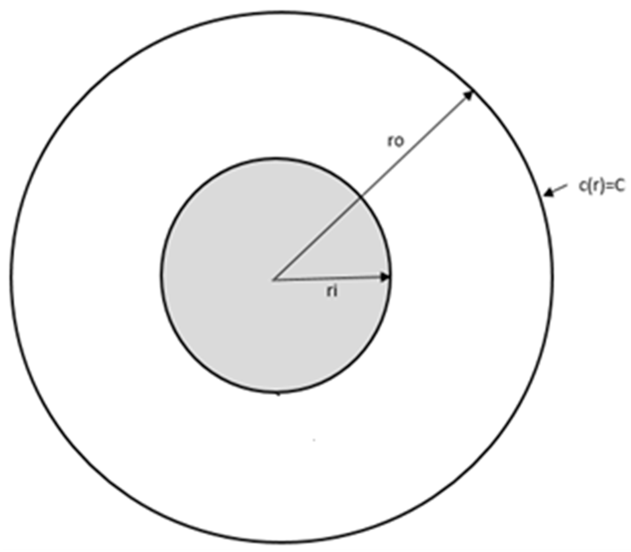
To verify that the MFS methodology solves the Laplace equation correctly for the given boundary conditions, an analytical solution for concentration distribution between the two concentric rigid cylinders is developed. This simplified set up reflects diffusion toward the surface of a single fiber where the chemical reaction occurs. A diagram of this test case is shown in Figure 2. In 1-D cylindrical coordinates, Laplace’s equation is written as follows:

$$0=\frac{1}{r} \frac{\partial }{\partial r}\left(r\frac{\partial c}{\partial r}\right)$$

(13)

Here, the outer cylinder surface has a known constant concentration, and the inner cylinder, representing an isolated fiber, is a reaction boundary, as described by (7) (see Figure 2). The analytical solution of the above equation with these boundary conditions is given as follows:

$$c\left(r\right)=\frac{C}{\frac{D}{k}\frac{1}{ r_i}+\ln \left(\frac{r_o}{r_i}\right)}\left(\frac{D}{k}\frac{1}{r_i}+\ln \left(\frac{r}{r_i}\right)\right),$$

(14)

where C is the constant concentration at the outer cylinder surface, D is the diffusion coefficient, k is the reaction rate constant, and r_i and r_o represent the inner and outer radius of the cylindrical surfaces, respectively.

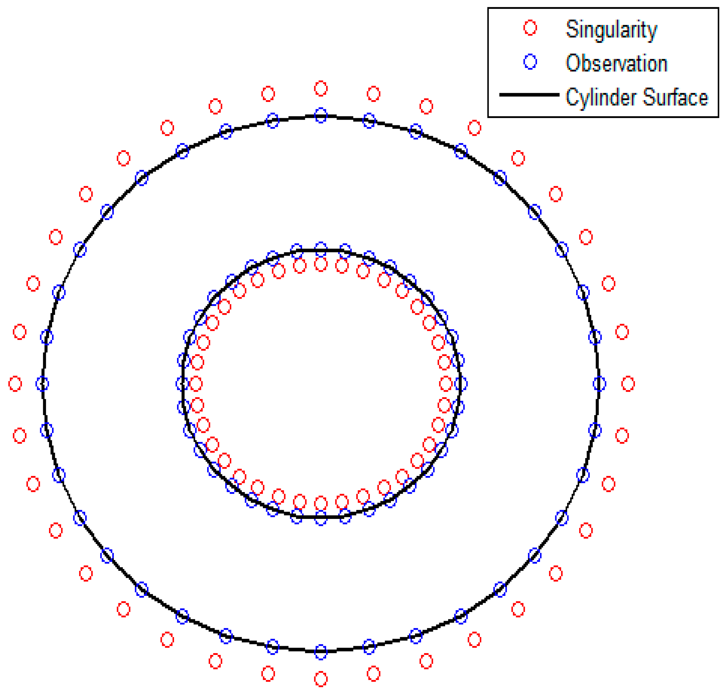
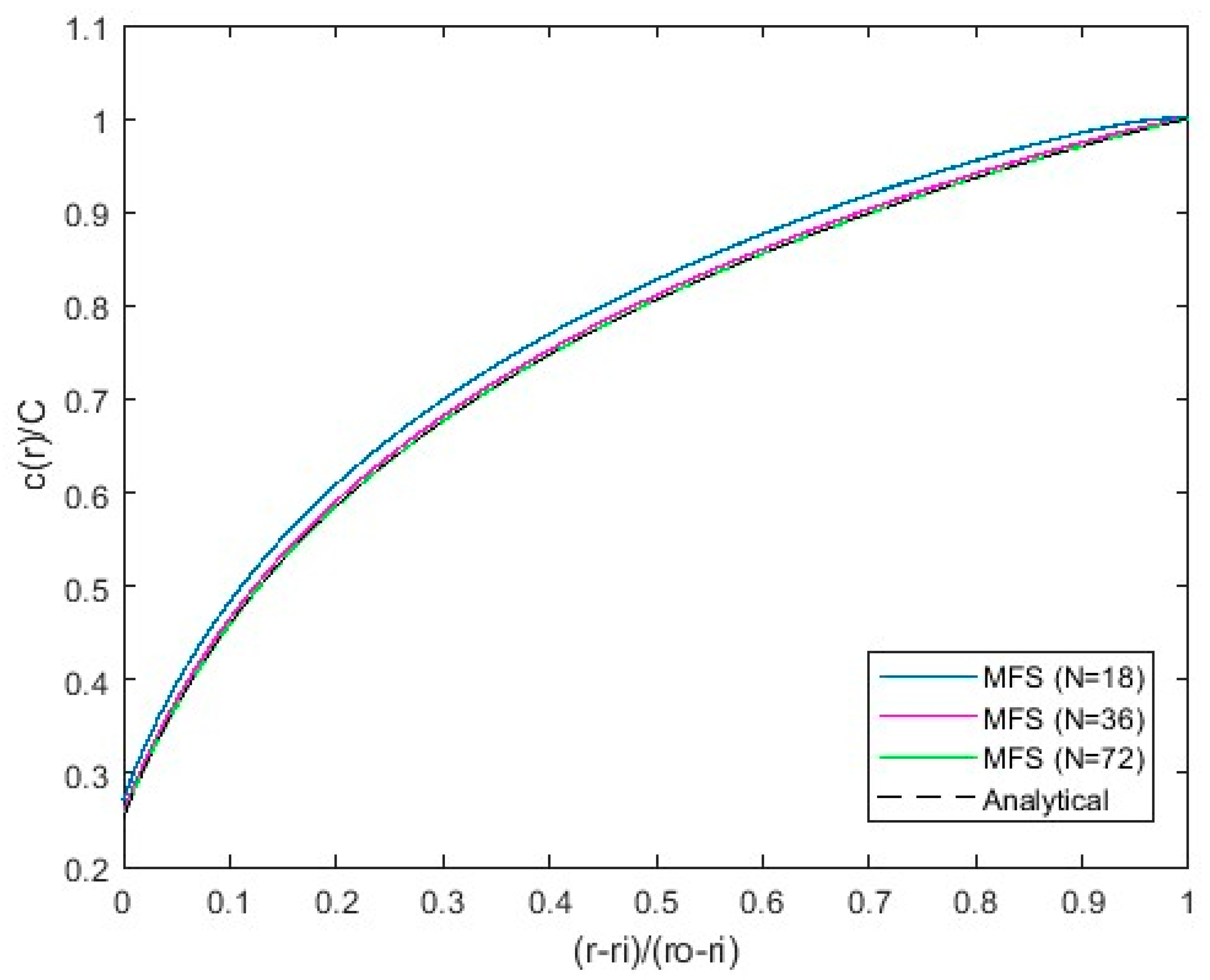
The set up of the 2-D MFS solution for the same geometry is shown in Figure 3. The red markers show the location of the singularities, and the blue markers represent observation points where the boundary conditions are set up. The observation points are placed on the inner and outer cylinders while the singularities are placed inside the cylinders at a submergence depth of 0.1 r, where r is the radius of the inner or outer cylinder in correspondence. The number of singular points and collocation points is the same. The analytical solution (14) and the MFS solution calculated using Green’s free space function for the Laplace operator with corresponding boundary conditions (5, 12) are shown in Figure 4.

The MFS computations with N = 18, 36 and 72 Stokeslets per cylinder surface are shown in Figure 4. Each surface has an equal number of observation points and Stokeslets. The obtained c(r) for N = 36 and N = 72 Stokeslets per cylinder practically coincide with each other and with the analytical solution (14). The number of observation points and singularities per fiber, N_f = 36, is therefore used in the computations in the next section.

After the steady MFS solution for the concentration of a given geometry of fibers with deposited film has been calculated, the concentration of the reactant at the fiber’s surface can then be used to calculate the growth rate [14] of deposited material before proceeding to the next time step. The CVD model [16] considers C₂H₂ as a precursor species of decomposed MTS in the gas phase, where the C₂H₂ concentration determines the SiC film formation rate. After calculating the concentration at the wall using (7), the growth rate of the fiber could then be calculated as follows by multiplying the concentration at the wall, calculating the reaction rate using the Arrhenius Equation (8), and determining the ratio of the molar mass ($M_{reactant}$) to the density of deposited film (${\rho }_{film})$:

$$\delta =2 \frac{M_{film}}{{\rho }_{film}}· k·c_{wall} ,$$

(15)

where $\delta$ is the growth rate of the fiber and $c_{wall}$ is the surface molar concentration of C₂H₂ at the wall in mol/m².

The density of SiC film is ρ_SiC = 3210 kg/m³ [16]. Coefficient 2 in the above formula appears because, by Equation (6), two molecules of SiC are synthesized by a single C₂H₂ molecule and the reaction rate is calculated by the concentration of C₂H₂ in Equations (7) and (8). The new location of the deposited surface is obtained by adding the deposited layer thickness, $\delta \Delta t,$ in the normal direction to the fiber.

Void tracking is an important part of modeling CVI. Figure 5 shows a depiction of a void. The area outlined in red is not accessible to reactant gas. The void-forming fiber surfaces do not continue to grow during the rest of the simulation. To determine the location of these voids, the computational domain is meshed. The concentration at boundaries where C > 0 is then set to 1 and any mesh point within a fiber is assumed to be a C = 0 boundary condition. The Laplace operator (3) for the concentration is then solved using a finite-difference scheme. After the solution has converged, any mesh point with C > 0 has access to the reactant and is not in a void, while any mesh point with C = 0 is either part of the fiber or in an area surrounded by fibers and has no access to the reactant. Solving (3) using a finite difference scheme is performed entirely for void tracking purposes and is not used to calculate concentrations or growth rates within the computational domain. This is a similar method to that developed in [24].

Once the growth rate is obtained using (15), the singularity and observation points are moved in the normal direction to the local surface, and the MFS solution is repeated at the next time step. This process continues until either the sample has been fully infiltrated (porosity is no longer decreasing) or the specified end time is reached.

The porosity of the samples is calculated by generating 10,000 random points within the computational domain. Whether the generated point is within a fiber or not is determined using the fiber center and observation points. The number of total points in fibers divided by the total number of points is the specimen’s porosity. To determine the accuracy of this porosity measurement, a sample with a known 80% porosity is measured 30 times. The average of the measurements is 79.93%, which is close to 80% (known porosity). The porosity minimum and maximum are 79.23% and 80.73%, respectively. The 3-σ range is 78.73–81.27%.

This section introduced the Robin boundary condition to the MFS to solve the diffusion equation with a chemical deposition reaction at the surface. The numerical procedure is coupled with the model of growth of deposited solid film. The validation of this proposed approach by comparing it to an analytical solution was successful.

3. Computational Results and Discussion

To further verify the MFS’s ability to model Chemical Vapor Infiltration, comparisons are made to experimental snapshots (Figure 6) and the quantitative data of infiltrated geometry (

Table 1. Summary of experimental porosity data from simulations using MFS.

Specimen	Temperature, °C	Run Time, Hours	Initial Computed Porosity	Initial Experimental Porosity	Final Porosity Computed by MFS	Final Experimental Porosity
1	1200	25	0.6378	0.64	0.1445	0.13
2	1200	31	0.6751	0.67	0.1883	0.24
3	1100	30.5	0.6533	0.65	0.1474	0.16
4	1200	66	0.6661	0.67	0.1573	0.20
5	1200	50	0.6318	0.63	0.1273	0.11
6	1200	22	0.7020	0.70	0.2363	0.28

).

In general, “real-time” simulations of CVI experiments with the same number of fibers are not feasible at this time due to computational limitations and the complex asymmetrical nature of the fiber preforms used. To model a woven fiber preform using MFS, millions of singularities are required. The resulting matrix that would need to be solved to obtain the strength of these singularities would, as a result, be on the order of 10¹² entries. This would need to be performed multiple times as time progresses throughout the infiltration process. As a result, the set ups of fibers considered using computational techniques, such as unidirectional fiber-reinforced substrates, are simplified versions of the actual experiments [33].

A 3-D woven preform would need to be reduced to the hundreds of 2-D long cylinders, with the N_c of the diameter of 8 microns (see Figure 6) located in a computational domain representing a small section of the actual geometry. The total size S of the 2-D computational domain encompassing N_c cylindrical fibers with porosity f is given by the following expression:

$$S=N_c\pi D^2/\left(4\left(1-f\right)\right)$$

(16)

For N_c = 500 fibers used in computations with D = 8 μ and f = 0.7 (specimen #6 in Table 1), the size of the computational domain is S = 83,773 μ². When the number of fibers used in MFS computations is doubled or halved, the obtained computational final porosity does not change.

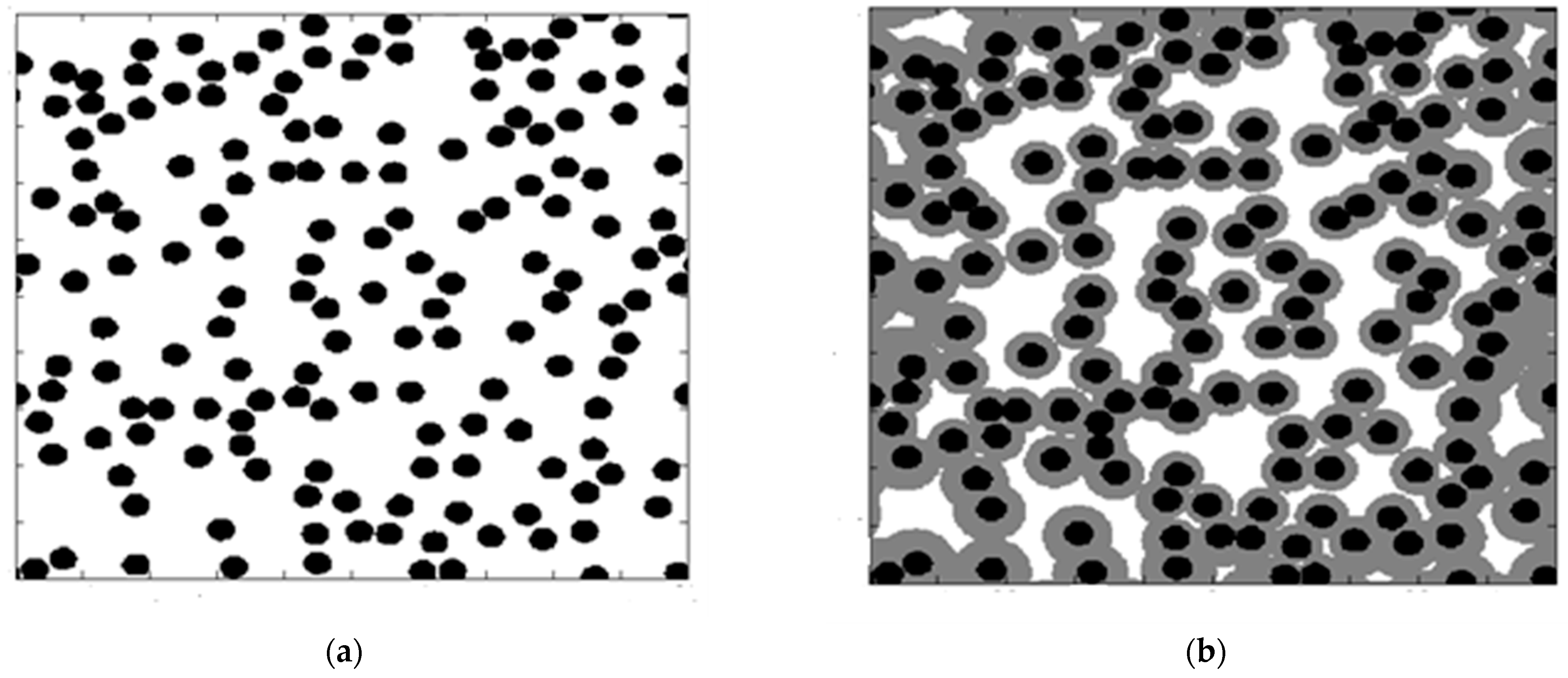
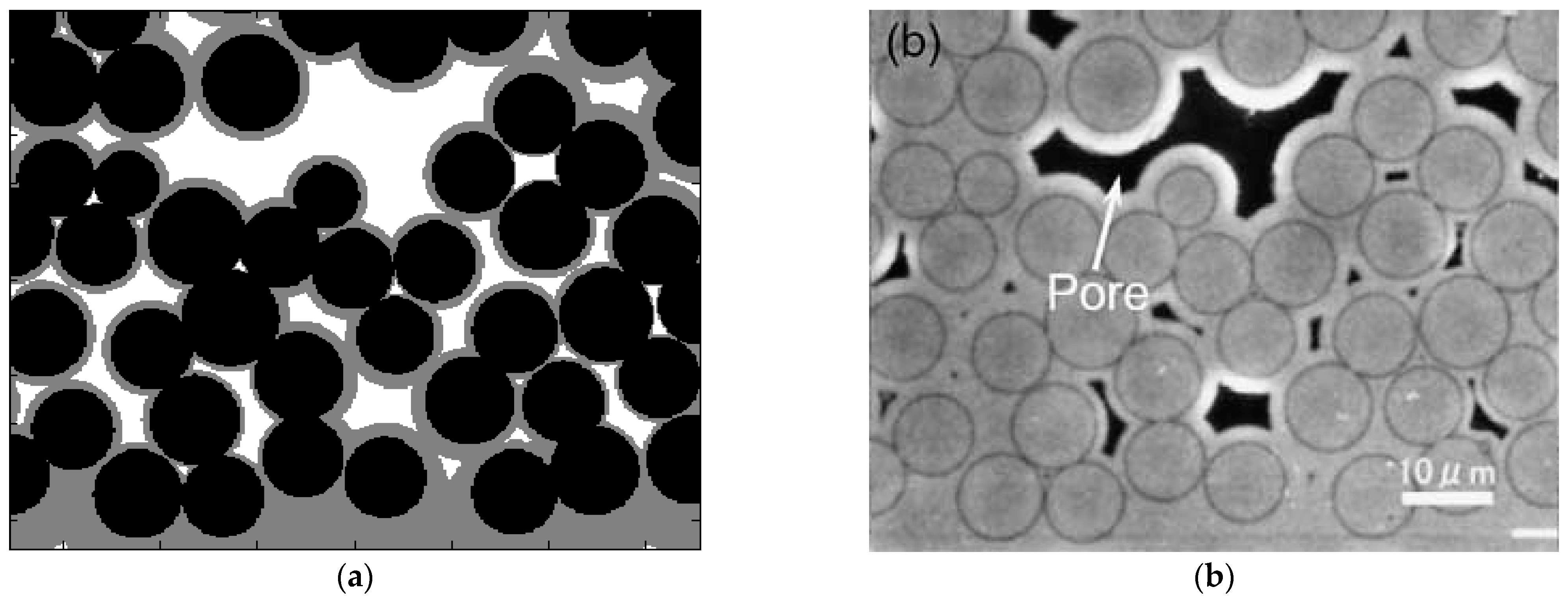
The computational results in Figure 6a are generated by simulating a small section of a woven geometry used in a CVI experiment using the same coordinates of the centers of fibers as those in the experiments depicted in Figure 6b. The obtained value of the diffusion coefficient, as outlined in Section 2, is D = 0.000528 m²/s at the conditions of experiments in [34], in which the preforms are infiltrated at 1100–1200 °C under atmospheric pressure.

In Ref. [35] the maximum SiC deposition rate is 9.5 nm/min. For MFS simulations, the chosen time step is Δt = 6 s to ensure the maximum deposition of ~1 nm per time step. This is a small added film thickness compared to ~8 microns diameter fibers (see Figure 6b) that justify the use of an explicit in-time approach to model the film deposition. The initial carbon interphase has a thickness ranging from 75 to 300 nm in experiments [34]. This layer was not accounted for in present MFS computations because the diameter of the fibers is much larger than the thickness of the initial carbon interface layer.

The initial porosity of this sample is 38.81%, and the final porosity after infiltration using MFS is 13.75%. A qualitative comparison of the computational results using MFS (Figure 6a) to the experimental results [35] (Figure 6b) is presented, showing a similar pattern of pores.

Figure 6. Comparison of infiltrated geometry (a) computed by MFS and (b) obtained experimentally, see [35], Figure 4, reprinted with Elsevier’s permission.

Figure 6. Comparison of infiltrated geometry (a) computed by MFS and (b) obtained experimentally, see [35], Figure 4, reprinted with Elsevier’s permission.

The results of the experiments [34] and the results of MFS simulations are shown in Table 1 in terms of the dynamics of porosity. The set ups of randomly generated circular fibers at different known porosities are generated by randomly placing fibers in the domain one at a time until the desired porosity is reached. The experimental conditions for specimen 4 in Table 1 [34] are mostly close to the results shown in Figure 6b [34].

The computations for listed specimens differ by initial porosity, run time, and temperature. If specimens differ by temperature, it affects the chemical reaction rate k in Equation (8). The initial porosities in computations are nearly identical to those in the experiments, as they should be. Slight differences between the initial experimental and computational porosities, ~0.005, are due to the computational porosity calculation and computational placement of fibers, as previously discussed.

After the geometry has infiltrated and computed using the MFS, the porosities of the experimental sample and the simulated domain compare well; see the last two columns of Table 1.

The final porosity for low-temperature case 3 is smaller in the experiments and in the MFS simulations as the faster kinetics close the outer surfaces faster at higher temperatures. Comparing case 1 with case 5 and case 2 with case 4 shows that the samples nearly reached terminal porosity after 25–30 h. Processing in similar conditions for double the time did not show a substantial change in the final porosity. To follow discussions in the experimental study [34], decreasing the initial average porosity was very effective at decreasing the final porosity. As a result, the average final porosity decreased in case 1 by decreasing the initial porosity compared to case 6. If the samples were ranked from the least porous to most porous after the MFS-modeled infiltration, the specimens’ order would be the same as the experiments (specimen 5, specimen 1, specimen 3, specimen 4, specimen 2, and specimen 6).

This section compared the MFS results to the experimentally obtained pattern of voids and the experimental porosity obtained for six different cases. There is a good correspondence of computational results obtained by the MFS with Robin boundary conditions to experimental data.

4. Conclusions

In the current study, the MFS method was developed and applied to the modeling of Chemical Vapor Infiltration (CVI) with a surface chemical reaction. The MFS method has not been used to solve CVI problems before. The concentrations of the reagent within the preform were obtained using Green’s free space functions for the Laplace operator, describing diffusion with boundary conditions corresponding to the CVI reaction at the fiber surfaces. For the quasi-equilibrium at the fiber surfaces considered, the reaction flux at the solid surface was equal to the diffusion flux towards the surface. To account for this condition, the Robin/third-type boundary condition at the fiber surfaces was developed and successfully incorporated with the MFS. These surface concentrations were used to calculate the fiber growth rate due to deposition. Comparisons of analytical solutions for the simplified geometry of two concentric cylinders mimicking a single fiber and MFS solution to the experimental snapshot of the fiber preforms with deposition are presented.

The dynamics of pore size and location were computed using the proposed MFS approach to evaluate the quality of the material obtained by CVI. Porosity transients were obtained for the range of initial porosities to show the relation between the initial and final porosities and the time needed to reach the final porosity.

The Method of Fundamental Solutions appears to be effective in modeling CVI with simplified one-step chemical surface reactions. The method accounts for circumferential variation in the deposition rate along the fiber’s surface, the depletion of the chemical reagent at part of the fiber’s surface, the merging of fibers with the formation of voids caused by deposition and the non-uniform distribution of the reactant throughout the domain. The present version of MFS was developed to simulate a CVI process that is isobaric and isothermal. The equality of reaction flux at the fiber’s surface and the diffusion flux towards the surface was assumed. Extensions of the proposed approach to more complex boundary conditions and the advection–diffusion equation will be addressed in future research.