Article

Testing Homogeneity of Proportion Ratios for Stratified Bilateral Correlated Data

Department of Biostatistics, University at Buffalo, Buffalo, NY 14214, USA
*
Author to whom correspondence should be addressed.
Math. Comput. Appl. 2024, 29(2), 26; https://doi.org/10.3390/mca29020026
Submission received: 9 January 2024 / Revised: 19 March 2024 / Accepted: 21 March 2024 / Published: 22 March 2024

Abstract

:
Intraclass correlation in bilateral data has been investigated in recent decades with various statistical methods. In practice, stratifying bilateral data by some control variables will provide more sophisticated statistical results to satisfy different research proposed in randomized clinical trials. In this article, we propose three test statistics (the likelihood ratio test, score test, and Wald-type test statistics) to evaluate the homogeneity of proportion ratios for stratified bilateral correlated data under an equal correlation assumption. Monte Carlo simulations of Type I error and power are performed, and the score test yields a robust outcome based on empirical Type I error and power. Lastly, two real data examples are conducted to illustrate the proposed three tests.

1. Introduction

In randomized clinical trials, bilateral data frequently occurs in patients who receive a treatment based on paired body parts or organs (such as eyes, ears, kidneys, and so on). Since the outcome of bilateral data has been naturally split into three types (no response, unilateral response, and bilateral responses), considering the intraclass correlation in the bilateral data is a natural way to avoid misleading results [1,2,3,4,5]. Intraclass correlation in bilateral data has been investigated in recent decades with various statistical methods [1,2,3,5,6,7,8]. Rosner proposes that the conditional probability of a response occurring at one side of paired body parts or organs that gives a response at the other body parts or organs is a positive constant R times the response rate [1]. Tang et al. provide a statistical inference for correlated data in binary paired data under the R model and also evaluate the asymptotic test with Type I error and power [9]. Ma, Shan, and Liu develop an asymptotic testing method under the homogeneity assumption for Rosner’s R model [5]. Donner assumes that all treatment groups share one intraclass correlation coefficient ρ [2], and Thompson evaluates the robustness of Donnar’s ρ model in pair data by adopting simulations [10]. Liu et al. test the equality of correlation coefficients based on Donner’s ρ model for paired binary data with multiple groups [11]. Later, Liu et al. explore the exact methods of testing the homogeneity of prevalence for correlated binary data under Donnar’s ρ model [8]. However, Dallal criticizes Rosner’s assumption and points out that “the constant R model will give a poor fit if the characteristic is almost certain to occur bilaterally with widely varying group-specific prevalence” [3]. He proposes that it is more advantageous to assume the characteristic emerges through a triggering mechanism, in which the probability of a subsequent occurrence is unaffected by the probability of initiating the trigger [3]. Dallal believes the conditional probability of a response at one side of paired body parts or organs giving a response at the other body parts or organs is a constant γ [3]. Li et al. develop asymptotic and exact methods following Dallal’s model [12]. Then, Chen et al. propose multiple test statistics of response rates in the different groups under Dallal’s model [13].
The homogeneity test for the appropriate effect size measure between different groups equates to testing the common value of the measure of effect. Moreover, there are three popular methods to evaluate the effect size in randomized clinical trials: the odds ratio, risk difference, and relative risk [14]. Indeed, relative risk is more informative than risk difference in some cases [15]. Compared with the odds ratio, the relative risk can process sparse data better. The stratifying of bilateral data by some control variables (e.g., disease phases, age, etc.) will provide more sophisticated statistical results to satisfy different research proposed in randomized clinical trials [16,17]. For example, evaluating the appropriate effect size across strata of disease phases between treatment and control groups equates to testing the effect size of homogeneity across the strata. Zhuang et al. investigate the homogeneity test of the ratio of two proportions in the stratified bilateral data based on Donner’s ρ model [18]. Shen et al. test the homogeneity of the difference between two proportions for stratified correlated paired binary data under Donner’s ρ model [19]. Xue and Ma propose interval estimation of proportion ratios for stratified bilateral correlated binary data under Rosner’s constant R model [20].
Rosner’s R and Donner’s ρ models have limitations and restrictions. Rosner’s R model is a conditional probability that a response at one side of paired body parts or organs that gives a response at the other body parts or organs is a positive constant R times the response rate [1]. However, the constant R can not reach one unless each response rate is equal, and the model is not appropriate if the patient’s body parts or organs are all responding and different groups have different response rates [3,20]. In Donner’s ρ model, it is assumed that all treatment groups share one intraclass correlation coefficient ρ [2]. However, when the correlations between the two groups are significantly different, Donner’s ρ model cannot be used for data analysis. In practice, it is first verified that the correlation coefficients are equal to decide whether the Donner model is appropriate. Compared to Rosner’s R and Donner’s ρ models, Dallal’s model does not require concern over whether all of a patient’s body parts or organs have responded, nor does it need to worry about whether different groups have varying response rates. Additionally, it eliminates the need to verify that the correlation coefficients are equal. Instead, it provides a straightforward intraclass correlation constant, γ , for the conditional probability of a response in one part of a pair of body parts or organs given a response in the other.
To avoid the limitations of Rosner’s R and Donner’s ρ models, we investigate the proportion ratios in clinical trial design with stratified bilateral data under Dallal’s model. The remainder of this paper is organized as follows: Section 2 presents the data structure and hypotheses, and Section 3 introduces the maximum-likelihood estimation under homogeneity. We propose three tests to examine the homogeneity of proportions across strata in Dallal’s model in Section 4. Accordingly, we investigate the performance and robustness of three tests by using simulation studies in Section 5. In Section 6, we use two real data examples to illustrate our proposed methods. Conclusions and future works are in Section 7.

2. Data Structure and Hypotheses

2.1. Notation

Let m l i j be the number of patients in the ith group of the jth stratum with lth responses, where i = 1, 2, j = 1 , , J , and l = 0, 1, 2. m + i j = m 0 i j + m 1 i j + m 2 i j represents the number of patients in the ith group of the jth stratum; p l i j corresponds to the probability of patients in the ith group of the jth stratum with lth responses. Define Z h i j k as the indicator of the response of the kth body parts or organs of the hth patient in the ith group from the jth stratum, where k = 1, 2 and h = 1 , 2 , , m + i j . If Z h i j k = 1 , then the improvement response occurs; otherwise, Z h i j k = 0 . Therefore, denote Pr Z h i j k = 1 = π i j , 0 π i j 1 as the probability of having response on one site. The corresponding data structure is shown in Table 1.
We explore the intraclass correlation based on Dallal’s model, where the conditional probability of a response at one side of paired body parts or organs, given a response at the other body parts or organs, is a constant γ . Therefore, we assume P Z h i j k = 1 Z h i j ( 3 k ) = 1 = γ j , and the probabilities of a body part or organ with none, one, or both can be expressed as follows:
p 0 i j = 1 2 γ j π i j ,
p 1 i j = 2 π i j 1 γ j ,
p 2 i j = π i j γ j ,
and p 0 i j + p 1 i j + p 2 i j = 1 for any fixed i and j. The joint likelihood function for the observed data m i j = m 0 i j , m 1 i j , m 2 i j T is given by
f m i j p i j = j = 1 J i = 1 2 m + i j ! m 0 i j ! m 1 i j ! m 2 i j ! p 0 i j m 0 i j p 1 i j m 1 i j p 2 i j m 2 i j ,
where p i j = p 0 i j , p 1 i j , p 2 i j T . The corresponding log-likelihood function can be expressed as:
l π i , γ = j = 1 J i = 1 2 m 0 i j log 1 2 γ j π i j + m 1 i j log 2 π i j 1 γ j + m 2 i j log π i j γ j + log C ,
where π i = π i 1 , , π i J T , γ = γ 1 , , γ J T and C = j = 1 J i = 1 2 m + i j ! m 0 i j ! m 1 i j ! m 2 i j ! is a constant.

2.2. Hypotheses for the Proportion Ratio across Strata

Assuming there is a common ratio of proportions between two groups across J strata, i.e., the ratio of proportions between two groups in the j th stratum is δ j = π 2 j / π 1 j for j = 1 , , J , the hypotheses are given as
H 0 : δ 1 = δ 2 = . . . = δ J versus H a : δ r δ s , for at least one pair of ( r , s ) , r s .

3. Maximum-Likelihood Estimation (MLE) under Homogeneity

3.1. The Constrained MLEs

Since we assume δ j = π 2 j / π 1 j for j = 1 , , J , then π 2 j = δ j π 1 j . Under the null hypothesis with a common δ , the log-likelihood function can be expressed as:
l π 1 , δ , γ = j = 1 J l j π 1 j , δ , γ j ,
where
l j π 1 j , δ , γ j = { m 01 j log 1 2 γ j π 1 j + m 11 j log 2 π 1 j 1 γ j + m 21 j log π 1 j γ j + m 02 j log 1 2 γ j π 1 j δ + m 12 j log 2 π 1 j δ 1 γ j + m 22 j log π 1 j δ γ j } + log C .
Differentiating l π 1 , δ , γ with respect to π 1 and γ , we have
l π 1 j = m 1 + j π 1 j + m 2 + j π 1 j + m 01 j γ j 2 π 1 j γ j 2 + 1 + δ m 02 j γ j 2 δ π 1 j γ j 2 + 1 ,
l γ j = m 21 j γ j + m 22 j γ j + m 11 j γ j 1 + m 12 j γ j 1 + m 01 j π 1 j π 1 j γ j 2 + 1 + δ m 02 j π 1 j δ π 1 j γ j 2 + 1 .
We can set l π 1 j = 0 with l γ j = 0 to obtain the MLEs π ^ 1 j and γ ^ j . Indeed, the MLE of γ j has a closed-form solution. Meanwhile, the MLE of π 1 j is a function of m l i j and δ . For the MLE of δ , we will update by using Fisher scoring iterative algorithm by consider the initial value of δ ( 0 ) as mean of unconstrained MLE δ ˜ j ( j = 1 J δ ˜ j J ), and
δ ^ = δ ( t + 1 ) = δ ( t ) + I 1 δ ( t ) l δ δ = δ ( t ) , π ^ 1 j , γ j ^ ,
where
l δ = j = 1 J ( m 12 j δ + m 22 j δ + m 02 j π 1 j γ j 2 δ π 1 j γ j 2 + 1 ) ,
2 l δ 2 = j = 1 J ( m 12 j δ 2 m 22 j δ 2 m 02 j π 1 j 2 γ j 2 2 δ π 1 j γ j 2 + 1 2 ) ,
and
I = E ( 2 l δ 2 ) = E ( j = 1 J ( m 12 j δ 2 m 22 j δ 2 m 02 j π 1 j 2 γ j 2 2 δ π 1 j γ j 2 + 1 2 ) ) = j = 1 J ( m + 2 j p 12 j δ 2 + m + 2 j p 22 j δ 2 + m + 2 j p 02 j π 1 j 2 γ j 2 2 δ π 1 j γ j 2 + 1 2 ) .

3.2. The Unconstrained MLEs

Under the alternative hypothesis, the log-likelihood can be presented as:
l π 1 , δ , γ = j = 1 J l j π 1 j , δ j , γ j ,
where
l j π 1 j , δ j , γ j = j = 1 J m 01 j log 1 2 γ j π 1 j + m 11 j log 2 π 1 j 1 γ j + m 21 j log π 1 j γ j + m 02 j log 1 2 γ j π 1 j δ j + m 12 j log 2 π 1 j δ j 1 γ j + m 22 j log π 1 j δ j γ j + log C ,
and the MLEs of three parameters, π 1 j , δ j , and γ j , can be derived by setting the partial differentiation equal to zero and then the MLEs as follows:
π ˜ 1 j = m 11 j + m 21 j m 11 j + m 12 j + 2 m 21 j + 2 m 22 j 2 m 01 j + m 11 j + m 21 j m 11 j + m 12 j + m 21 j + m 22 j ,
γ ˜ j = 2 m 2 + j m 1 + j + 2 m 2 + j ,
δ j ˜ = m 12 j + m 22 j m 01 j m 12 j + m 1 + j m 22 j + m 2 + j m 02 j + m 12 j + m 22 j m 12 j m 1 + j + m 22 j m 2 + j .

4. Testing Methods

4.1. Likelihood Ratio Test ( T L )

The likelihood ratio test statistic is given by
T L = 2 j = 1 J l j δ j ˜ , π ˜ 1 j , γ ˜ j l j δ ^ , π ^ 1 j , γ ^ j ,
Moreover, T L is asymptotically distributed as a Chi-square distribution with J 1 degrees of freedom under the null hypothesis. Then, reject the null hypothesis if T L > χ J 1 , 1 α 2 at a significant level α .

4.2. Score Test ( T S C )

Under the assumption that each stratum has the same ratio of proportions δ j ( δ = δ j ), the score test statistic is given by
T S C = j = 1 J U j I j 1 U j T δ = δ ^ , π 1 j = π ^ 1 j , γ j = γ ^ j = j = 1 J l j δ j 2 1 D j I j 1 ( 1 , 1 ) δ = δ ^ , π 1 j = π ^ 1 j , γ j = γ ^ j ,
I j 1 = 1 D j I 22 ( j ) I 33 ( j ) I 23 ( j ) I 32 ( j ) I 12 ( j ) I 33 ( j ) I 13 ( j ) I 32 ( j ) I 12 ( j ) I 23 ( j ) I 13 ( j ) I 22 ( j ) I 21 ( j ) I 33 ( j ) I 23 ( j ) I 31 ( j ) I 11 ( j ) I 33 ( j ) I 13 ( j ) I 31 ( j ) I 11 ( j ) I 23 ( j ) I 13 ( j ) I 21 ( j ) I 21 ( j ) I 32 ( j ) I 22 ( j ) I 31 ( j ) I 11 ( j ) I 32 ( j ) I 12 ( j ) I 31 ( j ) I 11 ( j ) I 22 ( j ) I 12 ( j ) I 21 ( j ) ,
D j = I 11 ( j ) I 22 ( j ) I 33 ( j ) I 11 ( j ) I 23 ( j ) I 32 ( j ) I 12 ( j ) I 21 ( j ) I 33 ( j ) + I 12 ( j ) I 23 ( j ) I 31 ( j ) + I 13 ( j ) I 21 ( j ) I 32 ( j ) I 13 ( j ) I 22 ( j ) I 31 ( j ) ,
where the score function for the j th stratum U j = l j δ , 0 , 0 and I j 1 ( 1 , 1 ) = I 22 ( j ) I 33 ( j ) I 23 ( j ) I 32 ( j ) is the first diagonal element of the inverse of the Fisher information matrix (see Appendix A for more detail). Therefore, T S C is asymptotically distributed as a Chi-square distribution with J 1 degrees of freedom under the null hypothesis. Then, reject the null hypothesis if T S C > χ J 1 , 1 α 2 at a significant level α .

4.3. Wald-Type Test ( T W )

An alternative way to express the null hypothesis is in matrix form as C β T = 0 , where
β = δ 1 , π 11 , γ 1 , δ 2 , π 12 , γ 2 , , δ J , π 1 J , γ J
and
C = 1 0 0 1 0 0 0 0 0 0 0 0 1 0 0 0 0 0 1 0 0 0 0 0 0 0 0 1 0 0 0 0 0 0 0 0 1 0 0 .
The information matrix for this Wald-type test I W is a 3 J × 3 J block diagonal matrix, with each block being a 3 × 3 information matrix of a parameter vector δ j , π 1 j , γ j within each stratum. We used the same derivation approach that we previously used to derive the information matrix for the score test.
I W = I W ( 1 ) 0 0 0 I W ( 2 ) 0 0 0 I W ( J ) 3 J × 3 J ,
with
I W ( j ) = I W 11 ( j ) I W 12 ( j ) I W 13 ( j ) I W 21 ( j ) I W 22 ( j ) I W 23 ( j ) I W 31 ( j ) I W 32 ( j ) I W 33 ( j ) 3 × 3 ,
where the explicit form of each element I W i k ( j ) is exactly the same as I i k j , derived in the score test. Then, the Wald-type test statistic can be expressed as:
T W = β C T C I W 1 C T 1 C β T β = δ ˜ 1 , , δ ˜ J , π ˜ 11 , , π ˜ 1 J , γ ˜ 1 , , γ ˜ J
I W 1 = I W ( 1 ) 1 0 0 0 I W ( 2 ) 1 0 0 0 I W ( J ) 1 J × J ,
where
( I W ( j ) ) 1 = 1 D W ( j ) I W 22 ( j ) I W 33 ( j ) I W 23 ( j ) I W 32 ( j ) I W 12 ( j ) I W 33 ( j ) I W 13 ( j ) I W 32 ( j ) I W 12 ( j ) I W 23 ( j ) I W 13 ( j ) I W 22 ( j ) I W 21 ( j ) I W 33 ( j ) I W 23 ( j ) I W 31 ( j ) I W 11 ( j ) I W 33 ( j ) I W 13 ( j ) I W 31 ( j ) I W 11 ( j ) I W 23 ( j ) I W 13 ( j ) I W 21 ( j ) I W 21 ( j ) I W 32 ( j ) I W 22 ( j ) I W 31 ( j ) I W 11 ( j ) I W 32 ( j ) I W 12 ( j ) I W 31 ( j ) I W 11 ( j ) I W 22 ( j ) I W 12 ( j ) I W 21 ( j ) ,
D W ( j ) = I W 11 ( j ) I W 22 ( j ) I W 33 ( j ) I W 11 ( j ) I W 23 ( j ) I W 32 ( j ) I W 12 ( j ) I W 21 ( j ) I W 33 ( j ) + I W 12 ( j ) I W 23 ( j ) I W 31 ( j ) + I W 13 ( j ) I W 21 ( j ) I W 32 ( j ) I W 13 ( j ) I W 22 ( j ) I W 31 ( j ) .
Meanwhile, T W is asymptotically distributed as a Chi-square distribution with J 1 degrees of freedom under the null hypothesis. Then, reject the null hypothesis if T W > χ J 1 , 1 α 2 at a significant level α .

5. Simulation Studies

This section investigates the empirical performances of three proposed test statistics in the previous section by three Monte Carlo simulation studies to evaluate the quality of relative risk in terms of the empirical Type I error rate and the power.

5.1. Empirical Type I Error Rates

In the first Monte Carlo simulation study, we investigate the behavior of the empirical Type I rate for three proposed tests under various procedures, where m = 25, 50, or 100 in strata J = 2, 4, 6, or 8. By considering that π 1 j and γ j are either common or different cross strata, we provide the parameter settings under different sample sizes and various sets of parameters in Table 2. For each configuration, 50,000 replications are randomly generated under the null hypothesis H 0 : δ = 1, 1.2, and 0.8, and the empirical Type I error rates are calculated by dividing the number of rejections by 50,000, and the nominal significant level α = 0.05. According to the previous study [9,20], the robustness of empirical Type I error rates is in the range from 0.04 to 0.06. In Table 3 and Appendix A.3 Table A1, Table A2 and Table A3, we observe that the Wald-type test has poor performance, and the likelihood ratio test does not work well under a small sample with multiple strata. However, the score test is more robust than the likelihood ratio and Wald-type test.
To obtain completed and robust empirical performances of the three proposed tests, we propose the second simulation by randomly choosing parameter configurations. We randomly generate 1000 parameter configurations within a parameter space for different sample sizes m = 15, 25, 50, 100 and a variety of strata J = 2, 4, 6, and 8 for 50,000 replications. Just as for the first simulation, the empirical Type I error rates can be calculated as the number of rejections divided by 50,000. Furthermore, the corresponding box plots and violin plots are shown in Figure 1, Figure 2, Figure 3 and Figure 4. Comparing empirical Type I error rates among the three tests, the score and likelihood ratio tests are stable and robust under all conditions. Still, the Wald-type test performs poorly compared to the other two tests. Indeed, the accuracy of the Wald-type test improves with larger sample sizes. The Wald-type test may perform poorly in small samples, leading to inaccurate p-values.

5.2. Power

The third Monte Carlo simulation aims to investigate the power performance among the three proposed tests. Based on the alternative hypothesis with respect to δ = H a 1 , H a 2 , and H a 3 , we consider the same strata, sample size, and parameter setting (Table 2) as in the first Monte Carlo simulation of the empirical Type I error. As the sample size increases, the powers of the three proposed tests increase for all strata settings (Figure 5, Figure 6, Figure 7 and Figure 8). In addition, as the strata increase, the powers increase for the three proposed tests. Considering the empirical Type I error, using the score test is highly recommended.

6. Real Data Examples

Two randomized clinical trial data are used as real data examples to illustrate the proposed three tests. The first real data example is a double-blinded randomized clinical trial data proposed by Mandel et al. [21]. In this clinical trial, children who suffer from otitis media with effusion (OME) and simultaneously have bilateral tympanocentesis are randomized into two groups: receiving 14-day treatments of amoxicillin or cefaclor [21]. After the treatment, the number of cured ears is summarized in Table 4 with the age group as strata. To explore whether the cured rates between the two groups (amoxicillin and cefaclor) among age strata are clinically equivalent, we test the homogeneity based on the three proposed tests. The MLEs of the parameters, based on observed data, are listed in Table 5, and the three test statistics and p-values are summarized in Table 6. However, all of the p-values are greater than 0.05, which means there is no statistical evidence to reject the null hypothesis H 0 : δ 1 = δ 2 = δ 3 .
Another example used to illustrate the three proposed tests is a randomized double-blinded placebo-controlled trial presented by Postlethwaite et al. [22]. In this trial, the primary measurement is the modified Rodnan Skin Score (MRSS), and patients diagnosed with diffuse scleroderma were randomly divided into the treatment and the control group. The duration of the disease (early or late phase) was considered two separate strata. Meanwhile, the number of improved hands is summarized by groups and disease phases in Table 7. We obtain the MLEs of the parameters in Table 8, and the statistics and p-values are summarized in Table 9. All of the p-values are greater than 0.05, which means there is no statistical evidence to reject the null hypothesis H 0 : δ 1 = δ 2 .

7. Conclusions

This article utilizes three MLE-based tests (LRT, Wald-type test, and score test) to test the homogeneity relative risk of two proportions on stratified bilateral correlated data.
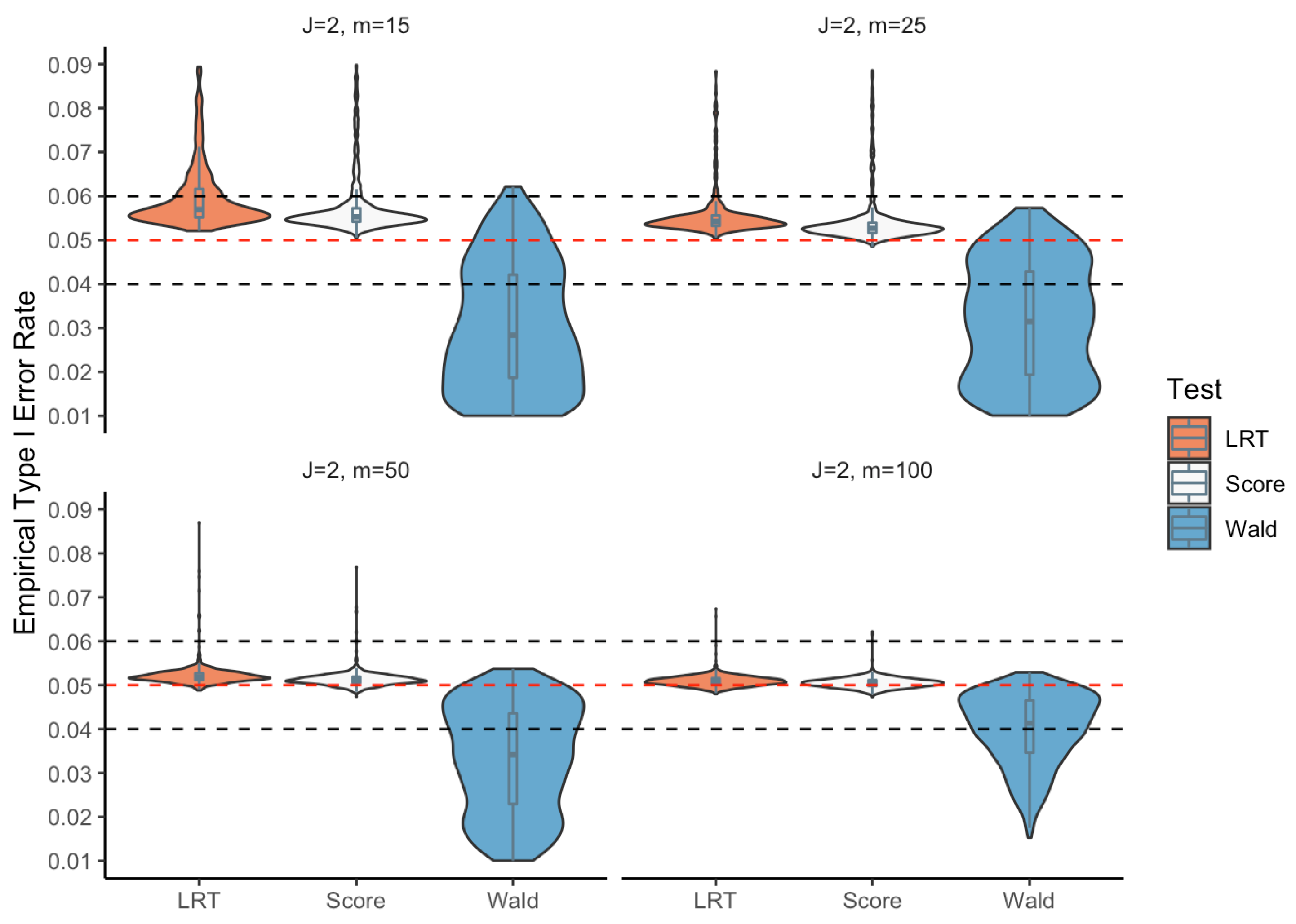
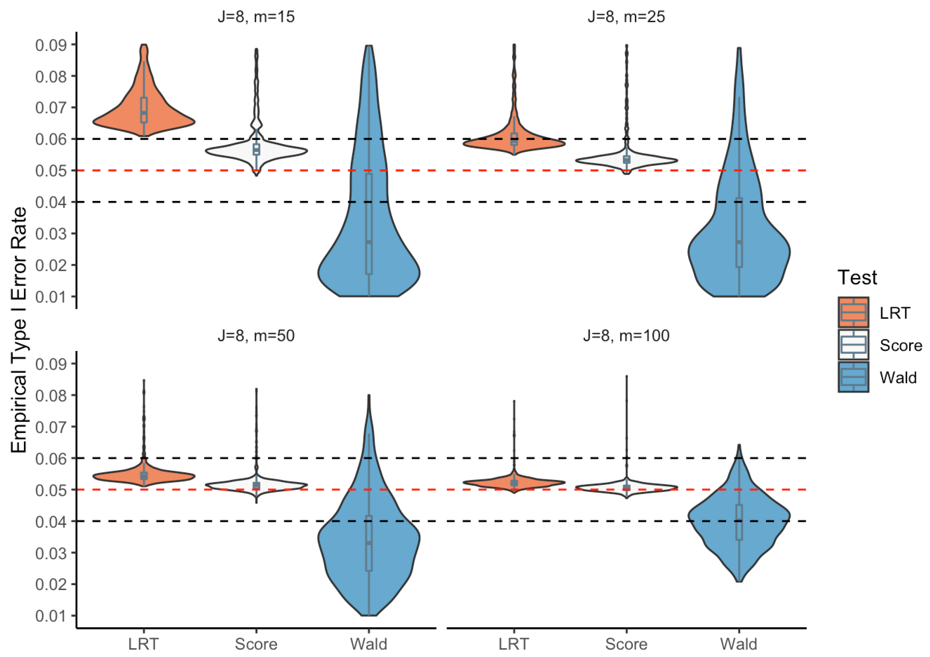
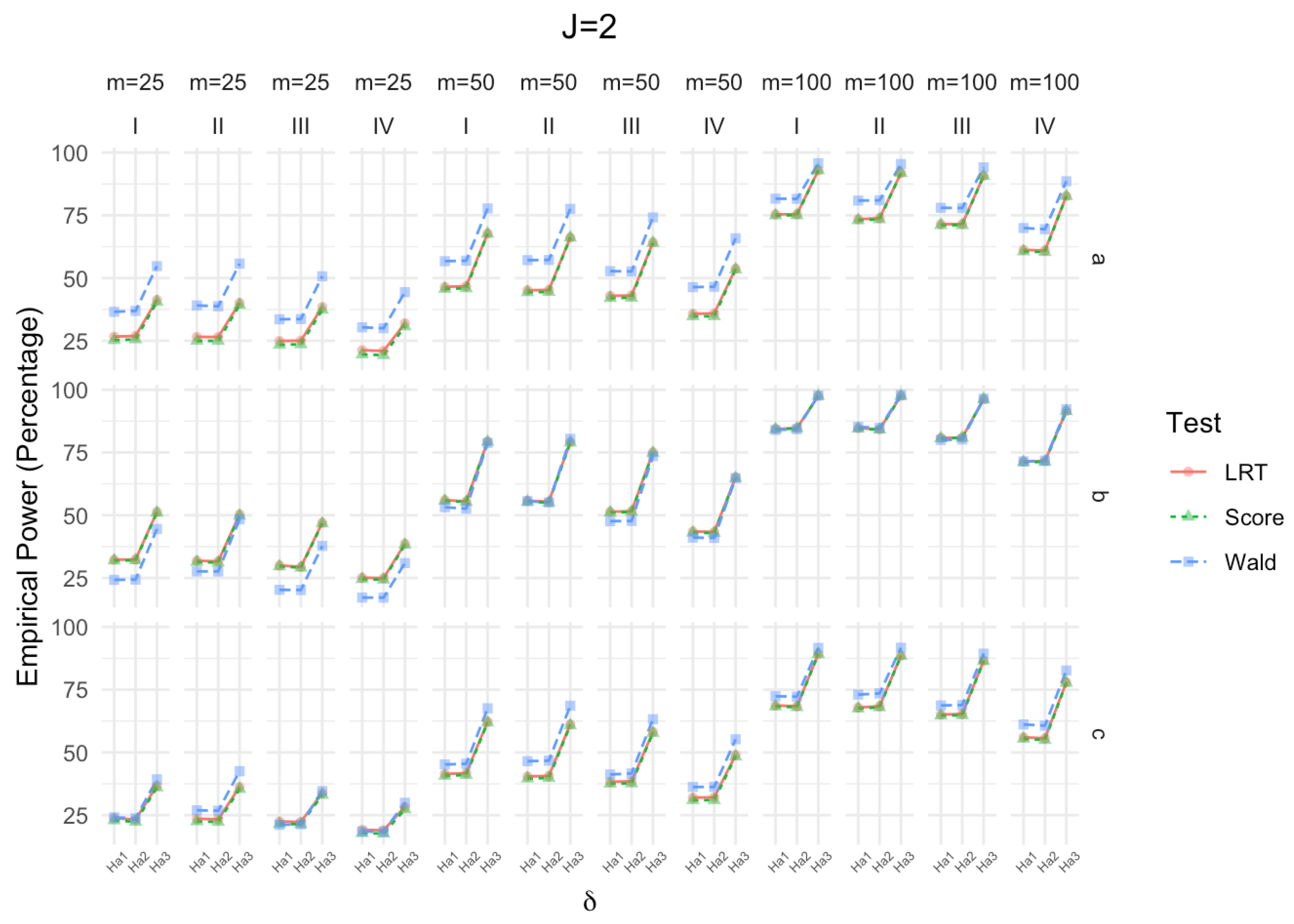
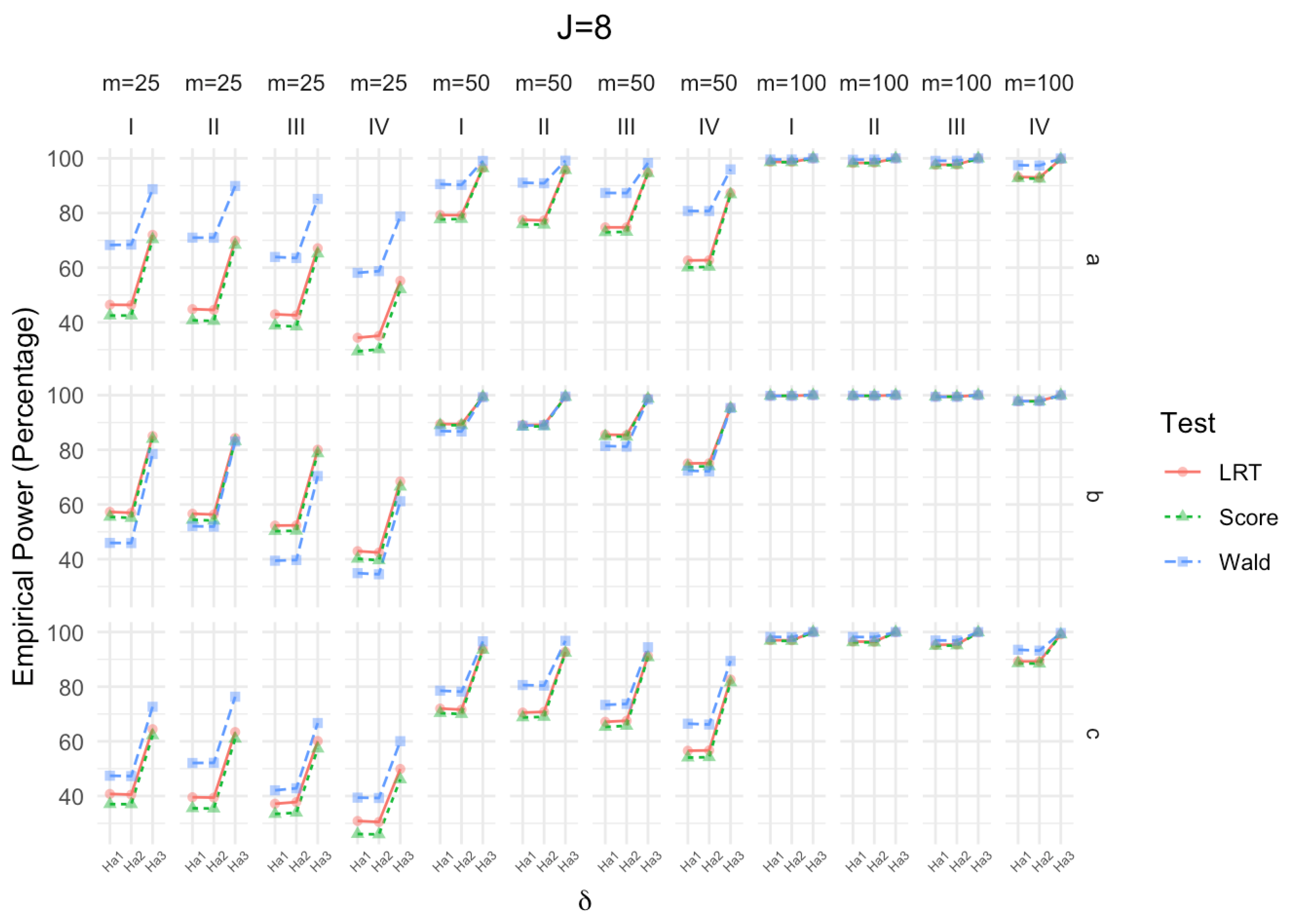
The three Monte Carlo simulation results show that the score test yields a robust performance with the empirical Type I error and power. Even with a small sample size and multiple strata, the score test still generates a stable empirical Type I error and satisfactory power. Meanwhile, the likelihood ratio test and Wald-type test offer reasonable power but come with unstable empirical Type I error performances. By incorporating a small sample size, the Wald-type test shows unsatisfactory performance of the empirical Type I error, but the performance tends to be reasonable by increasing the sample size. Under a small sample size with multiple strata, the score test is slightly unstable, but the performance also tends to be robust by increasing the sample size.
However, asymptotic methods may have some limitations due to poor performance under a small sample size with multiple strata. Future work might consider exact tests to investigate related issues.

Author Contributions

Conceptualization, W.T. and C.M.; Methodology, W.T. and C.M.; Writing—Original Draft Preparation, W.T.; Writing—Review & Editing, W.T. and C.M. All authors have read and agreed to the published version of the manuscript.

Funding

This research received no external funding.

Data Availability Statement

Data supporting this study are included within the article.

Conflicts of Interest

The authors declare no conflicts of interest.

Appendix A

Appendix A.1. Derivation of Score Statistic

The first-order differential equations of stratum j are:
l j δ = m 12 j δ + m 22 j δ + m 02 j π 1 j γ j 2 δ π 1 j γ j 2 + 1 ,
l j π 1 j = m 12 j π 1 j + m 21 j π 1 j + m 22 j π 1 j + m 01 j γ j 2 π 1 j γ j 2 + 1 + δ m 02 j γ j 2 δ π 1 j γ j 2 + 1 + m 11 j 2 γ j 2 2 π 1 j γ j 1 ,
l j γ j = m 21 j γ j + m 22 j γ j + m 11 j γ j 1 + m 12 j γ j 1 + m 01 j π 1 j π 1 j γ j 2 + 1 + δ m 02 j π 1 j δ π 1 j γ j 2 + 1 .
The second-order differential equations of stratum j are:
2 l j δ 2 = m 12 j δ 2 m 22 j δ 2 m 02 j π 1 j 2 γ j 2 2 δ π 1 j γ j 2 + 1 2 ,
2 l j δ π 1 j = m 02 j γ j 2 δ π 1 j γ j 2 + 1 δ m 02 j π 1 j γ j 2 2 δ π 1 j γ j 2 + 1 2 ,
2 l j δ γ j = m 02 j π 1 j δ π 1 j γ j 2 + 1 δ m 02 j π 1 j 2 γ j 2 δ π 1 j γ j 2 + 1 2 ,
2 l j π 1 j δ = m 02 j γ j 2 δ π 1 j γ j 2 + 1 δ m 02 j π 1 j γ j 2 2 δ π 1 j γ j 2 + 1 2 ,
2 l j π 1 j 2 = m 12 j π 1 j 2 m 21 j π 1 j 2 m 22 j π 1 j 2 m 01 j γ j 2 2 π 1 j γ j 2 + 1 2 δ 2 m 02 j γ j 2 2 δ π 1 j γ j 2 + 1 2 m 11 j 2 γ j 2 2 π 1 j 2 γ j 1 ,
2 l j π 1 j γ j = m 01 j π 1 j γ j 2 + 1 2 + δ m 02 j δ π 1 j γ j 2 + 1 2 ,
2 l j γ j δ = m 02 j π 1 j δ π 1 j γ j 2 + 1 δ m 02 j π 1 j 2 γ j 2 δ π 1 j γ j 2 + 1 2 ,
2 l j γ j π 1 j m 01 j π 1 j γ j 2 + 1 2 + δ m 02 j π 1 j 2 δ δ γ j 1 2 ,
2 l j γ j 2 = m 21 j γ j 2 m 22 j γ j 2 m 11 j γ j 1 2 m 12 j γ j 1 2 m 01 j π 1 j 2 π 1 j γ j 2 + 1 2 δ 2 m 02 j π 1 j 2 δ π 1 j γ j 2 + 1 2 .
The Fisher information of stratum j is:
I 11 ( j ) = E 2 l j δ 2 = m + 2 j δ 2 δ π 1 j γ j 2 + 1 m + 2 j δ 2 ,
I 12 ( j ) = I 21 ( j ) = E 2 l j δ π 1 j = m + 2 j γ j 2 δ π 1 j γ j 2 + 1 ,
I 13 ( j ) = I 31 ( j ) = E 2 l j δ γ j = m + 2 j π 1 j δ π 1 j γ j 2 + 1 ,
I 22 ( j ) = E 2 l j π 1 j 2 = m + 1 j γ j 2 2 π 1 j γ j 2 + 1 γ j 2 m + 1 j + δ m + 2 j π 1 j δ 2 m + 2 j γ j 2 2 π 1 j 2 δ δ γ j 1 ,
I 23 ( j ) = I 32 ( j ) = E 2 l j π 1 j γ j = δ m + 2 j π 1 j 2 δ δ γ j 1 m + 1 j π 1 j γ j 2 + 1 ,
I 33 ( j ) = E 2 l j γ j 2 = m + 1 j π 1 j γ j 2 m + 1 j π 1 j γ j 1 + m + 1 j π 1 j 2 π 1 j γ j 2 + 1 + δ 2 m + 2 j π 1 j 2 δ π 1 j γ j 2 + 1 + δ m + 2 j π 1 j γ j 2 δ m + 2 j π 1 j γ j 1 .

Appendix A.2. Derivation of Wald-Type Statistic

The first-order differential equations of stratum j are:
l j δ j = m 12 j δ j + m 22 j δ j + m 02 j π 1 j γ j 2 δ j π 1 j γ j 2 + 1 ,
l j π 1 j = m 12 j π 1 j + m 21 j π 1 j + m 22 j π 1 j + m 01 j γ j 2 π 1 j γ j 2 + 1 + δ j m 02 j γ j 2 δ j π 1 j γ j 2 + 1 + m 11 j 2 γ j 2 2 π 1 j γ j 1 ,
l j γ j = m 21 j γ j + m 22 j γ j + m 11 j γ j 1 + m 12 j γ j 1 + m 01 j π 1 j π 1 j γ j 2 + 1 + δ j m 02 j π 1 j δ j π 1 j γ j 2 + 1 .
The second-order differential equations of stratum j are:
2 l j δ j 2 = m 12 j δ j 2 m 22 j δ j 2 m 02 j π 1 j 2 γ j 2 2 δ j π 1 j γ j 2 + 1 2 ,
2 l j δ j π 1 j = m 02 j γ j 2 δ j π 1 j γ j 2 + 1 δ j m 02 j π 1 j γ j 2 2 δ j π 1 j γ j 2 + 1 2 ,
2 l j δ j γ j = m 02 j π 1 j δ j π 1 j γ j 2 + 1 δ j m 02 j π 1 j 2 γ j 2 δ j π 1 j γ j 2 + 1 2 ,
2 l j π 1 j δ j = m 02 j γ j 2 δ j π 1 j γ j 2 + 1 δ j m 02 j π 1 j γ j 2 2 δ j π 1 j γ j 2 + 1 2 ,
2 l j π 1 j 2 = m 12 j π 1 j 2 m 21 j π 1 j 2 m 22 j π 1 j 2 m 01 j γ j 2 2 π 1 j γ j 2 + 1 2 δ 2 m 02 j γ j 2 2 δ j π 1 j γ j 2 + 1 2 m 11 j 2 γ j 2 2 π 1 j 2 γ j 1 ,
2 l j π 1 j γ j = m 01 j π 1 j γ j 2 + 1 2 + δ j m 02 j δ j π 1 j γ j 2 + 1 2 ,
2 l j γ j δ j = m 02 j π 1 j δ j π 1 j γ j 2 + 1 δ j m 02 j π 1 j 2 γ j 2 δ j π 1 j γ j 2 + 1 2 ,
2 l j γ j π 1 j m 01 j π 1 j γ j 2 + 1 2 + δ j m 02 j π 1 j 2 δ j δ j γ j 1 2 ,
2 l j γ j 2 = m 21 j γ j 2 m 22 j γ j 2 m 11 j γ j 1 2 m 12 j γ j 1 2 m 01 j π 1 j 2 π 1 j γ j 2 + 1 2 δ 2 m 02 j π 1 j 2 δ j π 1 j γ j 2 + 1 2 .
The Fisher information of stratum j is:
I W 11 ( j ) = E 2 l j δ j 2 = m + 2 j δ j 2 δ j π 1 j γ j 2 + 1 m + 2 j δ j 2 ,
I W 12 ( j ) = I W 21 ( j ) = E 2 l j δ j π 1 j = m + 2 j γ j 2 δ j π 1 j γ j 2 + 1 ,
I W 13 ( j ) = I W 31 ( j ) = E 2 l j δ j γ j = m + 2 j π 1 j δ j π 1 j γ j 2 + 1 ,
I W 22 ( j ) = E 2 l j π 1 j 2 = m + 1 j γ j 2 2 π 1 j γ j 2 + 1 γ j 2 m + 1 j + δ j m + 2 j π 1 j δ j 2 m + 2 j γ j 2 2 π 1 j 2 δ j δ j γ j 1 ,
I W 23 ( j ) = I W 32 ( j ) = E 2 l j π 1 j γ j = δ j m + 2 j π 1 j 2 δ j δ j γ j 1 m + 1 j π 1 j γ j 2 + 1 ,
I W 33 ( j ) = E 2 l j γ j 2 = m + 1 j π 1 j γ j 2 m + 1 j π 1 j γ j 1 + m + 1 j π 1 j 2 π 1 j γ j 2 + 1 + δ j 2 m + 2 j π 1 j 2 δ j π 1 j γ j 2 + 1 + δ j m + 2 j π 1 j γ j 2 δ j m + 2 j π 1 j γ j 1 .

Appendix A.3. Empirical Type I Error Rates

Table A1. Simulation results of the empirical sizes (percentage) for 4 strata.
m = 25m = 50m = 100
δ γ π 1 T L T SC T W T L T SC T W T L T SC T W
1.0Ia5.825.454.335.335.174.355.075.034.59
b5.415.202.445.215.093.295.135.084.04
c5.735.462.495.315.203.195.115.054.00
IIa5.525.134.965.235.104.785.125.034.92
b5.545.282.415.235.123.275.125.074.06
c5.635.312.895.295.153.305.135.044.09
IIIa5.755.413.795.265.084.115.065.014.53
b5.525.302.395.054.933.145.055.013.91
c5.695.352.225.355.203.205.155.103.81
IVa5.595.164.055.235.004.555.195.104.64
b5.555.301.845.235.122.855.165.093.72
c5.775.332.435.365.183.015.155.083.75
1.2Ia5.675.343.675.265.104.165.175.084.51
b5.655.402.055.235.133.185.125.073.90
c5.655.351.965.265.132.905.215.143.74
IIa5.775.414.605.195.094.554.974.894.70
b5.545.321.925.345.192.965.205.174.02
c5.715.372.375.325.183.335.044.953.96
IIIa5.565.243.565.215.033.855.275.174.41
b5.455.211.865.415.263.075.175.113.85
c5.535.221.825.325.202.745.385.323.81
IVa5.725.264.005.305.134.114.964.884.38
b5.475.191.565.155.042.485.235.183.61
c5.785.371.925.295.132.845.415.303.65
0.8Ia5.565.234.865.245.034.665.165.074.71
b5.505.212.985.034.923.595.095.014.25
c5.775.342.985.245.063.375.245.164.18
IIa5.605.145.685.215.045.184.944.884.84
b5.535.232.875.375.233.645.145.084.22
c5.735.333.475.205.013.735.245.174.37
IIIa5.645.194.575.425.254.605.044.954.62
b5.635.342.965.435.273.765.095.044.19
c5.805.362.825.395.203.465.195.104.04
IVa5.835.245.105.385.154.905.155.064.78
b5.665.302.355.415.233.245.135.063.96
c5.755.123.025.335.073.365.024.893.79
Table A2. Simulation results of the empirical sizes (percentage) for 6 strata.
m = 25m = 50m = 100
δ γ π 1 T L T SC T W T L T SC T W T L T SC T W
1.0Ia5.905.474.775.305.114.555.064.994.63
b5.565.252.675.325.173.395.235.154.19
c5.895.492.805.375.173.315.175.073.95
IIa5.725.205.615.335.105.005.034.924.85
b5.575.272.545.505.323.455.115.053.97
c5.585.153.075.335.123.635.255.164.33
IIIa5.665.194.505.315.084.375.295.204.71
b5.795.412.575.335.173.405.145.054.00
c6.035.592.735.455.233.305.084.983.88
IVa5.985.385.215.385.134.725.145.014.73
b5.975.582.385.265.073.065.185.093.87
c5.915.272.935.315.043.405.265.153.91
1.2Ia5.795.344.145.285.044.245.225.134.55
b5.755.392.275.405.243.235.135.074.01
c5.565.192.325.605.443.245.245.163.78
IIa5.935.434.875.275.004.595.124.984.75
b5.835.472.115.144.973.025.115.033.92
c5.795.372.745.545.323.555.305.194.08
IIIa5.815.323.925.365.144.135.255.104.35
b5.685.332.155.375.233.055.155.103.81
c5.795.362.065.285.082.965.315.203.72
IVa5.965.424.485.214.924.375.275.174.62
b5.775.421.775.365.162.815.275.193.66
c5.745.212.285.585.323.175.365.263.84
0.8Ia5.975.445.715.234.995.015.215.115.17
b5.815.413.515.415.244.045.215.114.32
c6.065.463.695.214.993.655.155.064.29
IIa5.885.296.695.295.075.645.004.875.15
b5.695.323.415.285.093.835.024.934.21
c5.935.384.215.365.134.175.185.094.53
IIIa6.005.395.735.295.094.875.315.224.99
b5.905.523.495.255.073.675.325.214.41
c6.055.443.635.265.063.625.265.164.22
IVa6.245.466.315.435.095.455.355.195.09
b5.935.443.035.355.153.465.104.984.10
c6.145.344.215.435.113.935.245.104.18
Table A3. Simulation results of the empirical sizes (percentage) for 8 strata.
m = 25m = 50m = 100
δ γ π 1 T L T SC T W T L T SC T W T L T SC T W
1.0Ia5.875.395.015.405.154.725.024.914.68
b5.665.282.795.375.163.585.175.084.08
c6.045.513.065.405.193.685.165.064.03
IIa5.985.335.965.475.165.435.114.975.02
b5.625.192.645.365.193.545.135.043.99
c5.675.083.615.405.163.785.034.944.06
IIIa5.815.314.855.425.194.655.114.984.52
b5.805.382.835.134.943.245.245.154.06
c5.975.482.965.445.213.445.315.214.11
IVa5.905.215.685.535.235.075.315.164.90
b6.075.622.385.235.023.105.195.103.90
c6.195.453.455.445.183.635.205.084.04
1.2Ia5.955.374.265.375.124.385.275.144.72
b5.765.272.315.505.283.275.315.213.97
c5.845.362.355.395.153.155.435.334.06
IIa6.095.405.155.495.205.095.195.064.95
b5.725.292.125.204.983.025.135.033.90
c6.035.493.035.435.233.405.215.114.07
IIIa5.865.223.995.345.014.195.305.154.52
b5.715.282.185.405.263.115.185.104.00
c5.805.312.375.495.293.025.335.233.93
IVa5.825.224.935.435.154.625.124.984.63
b5.595.171.805.305.112.805.385.303.75
c6.015.382.585.525.233.305.255.103.83
0.8Ia6.105.486.345.395.125.465.165.015.15
b5.855.433.845.405.194.125.145.024.47
c5.835.234.215.355.084.115.044.944.23
IIa5.925.287.285.475.245.955.305.195.45
b5.775.323.695.335.143.945.205.114.25
c6.125.414.795.425.174.405.185.074.61
IIIa5.945.335.895.455.185.445.084.994.92
b5.795.283.775.565.324.045.235.134.43
c6.035.324.225.455.133.995.445.284.36
IVa6.305.387.315.485.125.705.205.045.29
b5.775.253.465.465.233.735.335.234.25
c6.355.364.695.485.144.365.375.184.51

References

  1. Rosner, B. Statistical methods in ophthalmology: An adjustment for the intraclass correlation between eyes. Biometrics 1982, 38, 105–114. [Google Scholar] [CrossRef]
  2. Donner, A. Statistical methods in ophthalmology: An adjusted chi-square approach. Biometrics 1989, 45, 605–611. [Google Scholar] [CrossRef]
  3. Dallal, G.E. Paired Bernoulli Trials. Biometrics 1988, 44, 253–257. [Google Scholar] [CrossRef] [PubMed]
  4. Ma, C.X.; Liu, S. Testing equality of proportions for correlated binary data in ophthalmologic studies. J. Biopharm. Stat. 2017, 27, 611–619. [Google Scholar] [CrossRef]
  5. Ma, C.X.; Shan, G.; Liu, S. Homogeneity test for binary correlated data. PLoS ONE 2015, 10, e0124337. [Google Scholar] [CrossRef]
  6. Tang, N.S.; Zhang, B.; Li, H.Q. Homogeneity test of difference between two correlated proportions in stratified matched-pair studies. J. Biopharm. Stat. 2013, 23, 1261–1280. [Google Scholar] [CrossRef] [PubMed]
  7. Tang, N.S.; Tang, M.L.; Qiu, S.F. Testing the equality of proportions for correlated otolaryngologic data. Comput. Stat. Data Anal. 2008, 52, 3719–3729. [Google Scholar] [CrossRef]
  8. Liu, X.; Shan, G.; Tian, L.; Ma, C.X. Exact methods for testing homogeneity of proportions for correlated multiple groups paired binary data. Commun. Stat. Comput. 2017, 46, 6074–6082. [Google Scholar] [CrossRef]
  9. Tang, M.L.; Tang, N.S.; Rosner, B. Statistical inference for correlated data in ophthalmologic studies. Stat. Med. 2006, 25, 2771–2783. [Google Scholar] [CrossRef] [PubMed]
  10. Thompson, J.R. The chi-square test for data collected on eyes. Br. J. Ophthalmol. 1993, 77. [Google Scholar] [CrossRef] [PubMed]
  11. Liu, X.; Liu, S.; Ma, C.X. Testing equality of correlation coefficients for paired binary data from multiple groups. Commun. Stat. Comput. 2015, 86, 1686–1696. [Google Scholar] [CrossRef]
  12. Li, Z.; Ma, C.; Ai, M. Statistical tests under Dallal’s model: Asymptotic and exact methods. PLoS ONE 2020, 15, e0242722. [Google Scholar] [CrossRef] [PubMed]
  13. Chen, Y.; Li, Z.; Ma, C. Further study on testing the equality of response rates under Dallal’s model. Stat. Interface 2022, 15, 115–126. [Google Scholar] [CrossRef]
  14. Newcombe, R.G. Confidence Intervals for Proportions and Related Measures of Effect Size; CRC Press: Boca Raton, FL, USA, 2012. [Google Scholar]
  15. Wang, W.; Shan, G. Exact confidence intervals for the relative risk and the odds ratio. Biometrics 2015, 71, 985–995. [Google Scholar] [CrossRef] [PubMed]
  16. Tang, N.S.; Qiu, S.F.; Tang, M.L.; Pei, Y.B. Asymptotic confidence interval construction for proportion difference in medical studies with bilateral data. Stat. Methods Med. Res. 2011, 20, 233–259. [Google Scholar] [CrossRef]
  17. Tang, N.S.; Qiu, S.F. Homogeneity test, sample size determination and interval construction of difference of two proportions in stratified bilateral-sample designs. J. Stat. Plan. Inference 2012, 142. [Google Scholar] [CrossRef]
  18. Zhuang, T.; Tian, G.L.; Ma, C.X. Homogeneity Test of Ratio of Two Proportions in Stratified Bilateral Data. Stat. Biopharm. Res. 2018, 11, 200–209. [Google Scholar] [CrossRef]
  19. Shen, X.; Ma, C.X. Testing homogeneity of difference of two proportions for stratified correlated paired binary data. J. Appl. Stat. 2018, 45, 1410–1425. [Google Scholar] [CrossRef]
  20. Xue, Y.; Ma, C.X. Interval estimation of proportion ratios for stratified bilateral correlated binary data. Stat. Methods Med. Res. 2020, 29, 1987–2014. [Google Scholar] [CrossRef]
  21. Mandel, E.M.; Bluestone, C.D.; Rockette, H.E.; Blatter, M.M.; Reisinger, K.S.; Wucher, F.P.; Harper, J. Duration of effusion after antibiotic treatment for acute otitis media: Comparison of cefaclor and amoxicillin. Pediatr. Infect. Dis. 1982, 1, 310–316. [Google Scholar] [CrossRef]
  22. Postlethwaite, A.E.; Wong, W.K.; Clements, P.; Chatterjee, S.; Fessler, B.J.; Kang, A.H.; Korn, J.; Mayes, M.; Merkel, P.A.; Molitor, J.A.; et al. A multicenter, randomized, double-blind, placebo-controlled trial of oral type I collagen treatment in patients with diffuse cutaneous systemic sclerosis: I. oral type I collagen does not improve skin in all patients, but may improve skin in late-phase disease. Arthritis Rheumatol. 2008, 58, 1810–1822. [Google Scholar]
Figure 1. Violin plots and box plots of empirical sizes ( J = 2 ).
Mca 29 00026 g001
Figure 2. Violin plots and box plots of empirical sizes ( J = 4 ).
Mca 29 00026 g002
Figure 3. Violin plots and box plots of empirical sizes ( J = 6 ).
Mca 29 00026 g003
Figure 4. Violin plots and box plots of empirical sizes ( J = 8 ).
Mca 29 00026 g004
Figure 5. Line plots of empirical power ( J = 2 ).
Mca 29 00026 g005
Figure 6. Line plots of empirical power ( J = 4 ).
Mca 29 00026 g006
Figure 7. Line plots of empirical power ( J = 6 ).
Mca 29 00026 g007
Figure 8. Line plots of empirical power ( J = 8 ).
Mca 29 00026 g008
Table 1. Data structure.
Group
Number of Responses (l)12Total
0 m 01 j ( p 01 j ) m 02 j ( p 02 j ) m 0 + j
1 m 11 j ( p 11 j ) m 12 j ( p 12 j ) m 1 + j
2 m 21 j ( p 21 j ) m 22 j ( p 22 j ) m 2 + j
Total m + 1 j m + 2 j m + + j
Table 2. Parameter setups for computing empirical Type I error rates and powers.
Number of Strata
ParameterCasesJ = 2J = 4J = 6J = 8
I(0.2, 0.4)(0.2, 0.4, 0.2, 0.4)(0.2, 0.4, 0.2, 0.4, 0.2, 0.4)(0.2, 0.4, 0.2, 0.4, 0.2, 0.4, 0.2, 0.4)
γ II(0.3, 0.3)(0.3, 0.3, 0.3, 0.3)(0.3, 0.3, 0.3, 0.3, 0.3, 0.3)(0.3, 0.3, 0.3, 0.3, 0.3, 0.3, 0.3, 0.3)
III(0.3, 0.5)(0.3, 0.5, 0.3, 0.5)(0.3, 0.5, 0.3, 0.5, 0.3, 0.5)(0.3, 0.5, 0.3, 0.5, 0.3, 0.5, 0.3, 0.5)
IV(0.6, 0.6)(0.6, 0.6, 0.6, 0.6)(0.6, 0.6, 0.6, 0.6, 0.6, 0.6)(0.6, 0.6, 0.6, 0.6, 0.6, 0.6, 0.6, 0.6)
π 1 a(0.2, 0.4)(0.2, 0.4, 0.2, 0.4)(0.2, 0.4, 0.2, 0.4, 0.2, 0.4)(0.2, 0.4, 0.2, 0.4, 0.2, 0.4, 0.2, 0.4)
b(0.3, 0.3)(0.3, 0.3, 0.3, 0.3)(0.3, 0.3, 0.3, 0.3, 0.3, 0.3)(0.3, 0.3, 0.3, 0.3, 0.3, 0.3, 0.3, 0.3)
c(0.2, 0.3)(0.2, 0.3, 0.2, 0.3)(0.2, 0.3, 0.2, 0.3, 0.2, 0.3)(0.2, 0.3, 0.2, 0.3, 0.2, 0.3, 0.2, 0.3)
δ H a 1 :(0.5, 1)(0.5, 1, 0.5, 1)(0.5, 1, 0.5, 1, 0.5, 1)(0.5, 1, 0.5, 1, 0.5, 1, 0.5, 1)
H a 2 (0.5, 1.2)(0.5, 1.2, 0.5, 1.2)(0.5, 1.2, 0.5, 1.2, 0.5, 1.2)(0.5, 1.2, 0.5, 1.2, 0.5, 1.2, 0.5, 1.2)
H a 3 (0.5, 1.4)(0.5, 1.4, 0.5, 1.4)(0.5, 1.4, 0.5, 1.4, 0.5, 1.4)(0.5, 1.4, 0.5, 1.4, 0.5, 1.4, 0.5, 1.4)
Table 3. Simulation results of the empirical sizes (percentage) for 2 strata.
m = 25m = 50m = 100
δ γ π 1 T L T SC T W T L T SC T W T L T SC T W
1.0Ia5.465.283.765.285.173.975.065.034.41
b5.395.372.045.285.233.405.095.074.20
c5.315.251.715.195.152.995.135.114.02
IIa5.655.434.685.355.234.455.275.224.73
b5.425.421.925.395.333.334.944.924.05
c5.545.462.395.225.163.235.105.084.00
IIIa5.365.213.425.335.243.925.145.104.27
b5.505.471.835.215.153.145.075.044.12
c5.415.291.525.145.112.795.115.093.87
IVa5.515.213.955.125.013.775.034.974.23
b5.495.441.205.225.202.794.944.903.78
c5.485.341.705.325.202.715.245.183.73
1.2Ia5.375.223.665.245.154.004.984.954.29
b5.545.481.705.165.103.155.065.044.08
c5.565.471.485.255.182.765.125.113.87
IIa5.425.294.475.115.064.285.145.104.70
b5.195.151.515.055.003.035.004.984.01
c5.495.442.175.115.073.155.075.043.91
IIIa5.255.133.325.084.993.635.095.054.27
b5.285.241.465.145.092.995.135.104.00
c5.535.461.315.295.252.564.884.863.65
IVa5.375.123.765.175.053.875.205.124.29
b5.625.571.055.125.092.485.265.243.84
c5.645.501.445.145.092.465.175.143.55
0.8Ia5.315.133.815.165.074.145.155.094.47
b5.365.332.495.155.103.605.105.064.34
c5.545.392.085.175.123.125.085.044.10
IIa5.405.144.635.205.084.345.095.034.63
b5.415.362.305.305.243.685.105.084.29
c5.295.142.455.255.183.394.994.954.00
IIIa5.455.283.775.205.113.955.125.064.42
b5.315.282.025.255.223.495.004.994.14
c5.295.181.755.265.172.955.195.123.98
IVa5.725.434.075.235.123.995.125.084.39
b5.435.341.555.305.263.025.014.983.84
c5.515.191.955.235.122.825.345.293.86
Table 4. Frequency of number of OME-free ears after treatment.
Age Group
<2 years2–5 years≥6 years
Number of OME-Free EarsCefactorAmoxicillinCefactorAmoxicillinCefactorAmoxicillin
08116301
1226110
28210536
Table 5. MLEs of parameters based on observed data (OME-free ears).
Unconstrained MLEsConstrained MLEs
Age Groups π ˜ 1 γ ˜ δ ˜ π ^ 1 γ ^ δ ^
<2 years0.47620.83330.48000.40360.83330.8174
2–5 years0.61160.81080.91670.62490.8108-
≥6 years0.95000.94740.85720.95000.9474-
Table 6. The values of statistics and p-values for three different tests (OME-free ears).
T L T SC T W
Statistic1.69181.63922.3520
P0.42920.44060.3085
Table 7. Number of patients with hand MRSS decreased.
EarlyLate
Number of Hands with ImprovementCollagenPlaceboCollagenPlacebo
02023922
12332
25432
Table 8. MLEs of parameters based on observed data (MRSS).
Unconstrained MLEsConstrained MLEs
Phase π ˜ 1 γ ˜ δ ˜ π ^ 1 γ ^ δ ^
Early0.2130.7830.9000.2480.7830.626
Late0.3000.6670.3850.2450.667-
Table 9. The values of statistics and p-values for three different tests (MRSS).
T L T SC T W
Statistic1.39791.39551.2046
P0.23710.23750.2724
Disclaimer/Publisher’s Note: The statements, opinions and data contained in all publications are solely those of the individual author(s) and contributor(s) and not of MDPI and/or the editor(s). MDPI and/or the editor(s) disclaim responsibility for any injury to people or property resulting from any ideas, methods, instructions or products referred to in the content.

