FE² Computations with Deep Neural Networks: Algorithmic Structure, Data Generation, and Implementation

Abstract

Multiscale FE${}^2$ computations enable the consideration of the micro-mechanical material structure in macroscopical simulations. However, these computations are very time-consuming because of numerous evaluations of a representative volume element, which represents the microstructure. In contrast, neural networks as machine learning methods are very fast to evaluate once they are trained. Even the DNN-FE${}^2$ approach is currently a known procedure, where deep neural networks (DNNs) are applied as a surrogate model of the representative volume element. In this contribution, however, a clear description of the algorithmic FE${}^2$ structure and the particular integration of deep neural networks are explained in detail. This comprises a suitable training strategy, where particular knowledge of the material behavior is considered to reduce the required amount of training data, a study of the amount of training data required for reliable FE${}^2$ simulations with special focus on the errors compared to conventional FE${}^2$ simulations, and the implementation aspect to gain considerable speed-up. As it is known, the Sobolev training and automatic differentiation increase data efficiency, prediction accuracy and speed-up in comparison to using two different neural networks for stress and tangent matrix prediction. To gain a significant speed-up of the FE${}^2$ computations, an efficient implementation of the trained neural network in a finite element code is provided. This is achieved by drawing on state-of-the-art high-performance computing libraries and just-in-time compilation yielding a maximum speed-up of a factor of more than 5000 compared to a reference FE${}^2$ computation. Moreover, the deep neural network surrogate model is able to overcome load-step size limitations of the RVE computations in step-size controlled computations.

1. Introduction

Nearly all commonly applied engineering materials possess, depending on the detail of investigation, some heterogeneous microstructure, e.g., fiber-reinforced polymers or rolled steel alloys, where the grains can have preferential directions because of the manufacturing process. Since this heterogeneous microstructure can significantly influence the response of these materials to mechanical loading, it is of particular interest to consider the microstructure already in numerical simulations. The development of constitutive models for materials with heterogeneous microstructures is challenging in both aspects, phenomenological constitutive modeling and subsequent experimental calibration. Thus, the so-called FE${}^2$ method has been developed by [1,2,3,4,5,6]—to mention only a few—for coupled numerical simulation of structures at macro- and microscale with finite elements. There, in contrast to common finite element computations, a constitutive model is not assigned to an integration point at macroscale. Instead, the stress and consistent tangent quantities are obtained by solving an initial boundary value problem with finite elements on a particular microstructure followed by a numerical homogenization technique. In this context, the microstructure is usually denoted as a representative volume element (RVE). In addition to the aforementioned works, in [7], a comprehensive description of the FE${}^2$-method for the numerical solution of these coupled boundary value problems on different scales is provided. In general, there exist further methods to obtain the response of heterogeneous microstructures, such as Discrete Fourier Transforms or Fast Fourier Transforms; see, for example, [8]. Even the finite cell method is applicable for the homogenization of heterogeneous microstructures; see, for example, [9]. However, in this work, deep neural networks are applied to replace the computationally costly solution of initial boundary value problems at microscale.

Currently, various applications of methods of artificial intelligence exist in the field of solid mechanics. A comprehensive overview of applications in continuum material mechanics is given in [10]. Further reviews are provided in [11,12] for applications in experimental solid mechanics and [13] for material development in additive manufacturing employing machine learning methods. Ref. [14] provides a general introduction to the application of machine learning techniques in material modeling and design of materials. Additionally, in [15], a review and investigation of the ability to apply machine learning in constitutive modeling is provided; however, it is in the context of soils. Most applications of machine learning methods aim to obtain feasible information from huge amounts of data or to increase the speed of particular computations. The source of the data could either be simulations, as in the present work, or directly experimental data, as in the data-driven mechanics approach, which was introduced by the aithors of [16], where it is not required to learn the response of constitutive models from simulations.

The application of artificial neural networks for data-based constitutive modeling was originally introduced in [17] and is frequently used in representing the material behavior for finite element simulations since then; see, for example, [18,19]. Recently, different approaches have been published to advance numerical simulations with machine learning methods. An investigation into deep learning surrogate models for accelerating numerical simulations is presented in [20]. Ref. [21] contains a proposal of a combination of physics-based finite element analysis and convolutional neural networks for predicting the mechanical response of materials. In contrast, ref. [22] contains an application of deep learning techniques for extracting rules that are inherent in computational mechanics to propose a new numerical quadrature rule that shows results superior to the well-known Gauss–Legendre quadrature.

Learning material behavior from simulations is generally covered with versatile approaches. In this context, the authors of [23] describe a material modeling framework for hyperelasticity and plasticity, where different architectures of neural networks are employed. Model-free procedures that fit into the data-driven mechanics approach for representing material behavior are described in [24,25,26,27], among others. Model-free approaches are suitable, especially for the consideration of elastoplastic material behavior; see [28,29] as well. Artificial neural networks could also be applied for calibrating known constitutive models from experimental data (parameter identification). First attempts are presented in [30,31], whereas  in [32], modern deep reinforcement learning techniques are applied for the calibration of history-dependent models. Since the measurement techniques to obtain experimental data have evolved in recent years, modern calibration techniques can consider full-field data, e.g., from digital image correlation; see [33]. Instead of calibrating constitutive models from experimental data with neural networks, where an error is introduced from choosing the constitutive model, the experimental data can be directly employed for discovering the material models from data. This approach is introduced in [34] for hyperelasticity and later on extended to cover elastoplasticity [35] and generalized materials [36]. Similar work with automated discovery of suitable hyperelastic materials is provided in [37], where constitutive artificial neural networks are applied, introduced in [38].

Many different machine learning methods are successfully used for multiscale applications in solid mechanics. There, the main objective is to obtain the homogenized response from heterogeneous microstructures. One of the first works in this context is provided in [39], wherein the authors applied neural networks for the homogenization of non-linear elastic materials. Ref. [40] contains a proposal of a data-driven two-scale approach to predict homogenized quantities even for inelastic deformations by drawing on clustering techniques. The ability to replace microscale evaluations with artificial neural networks requires a suitable accuracy of the network after the training process. Regarding this issue, the authors of ref. [41] make use of artificial neural networks as constitutive relation surrogates for nonlinear material behavior. However, based on the evaluation of quality indicators, a reduced-order model can be employed instead of the neural network within an adaptive switching method. The authors of ref. [42] describe the so-called Structural-Genome-Driven approach for FE${}^2$computations of composite structures, wherein even model reduction techniques are applied.

Advanced neural network architectures such as convolutional or recurrent neural networks are regularly applied to predict the homogenized response of microstructures. Here, atomistic data can also be used showing significant acceleration compared to molecular statics [43]. Elastic material behavior is investigated in [44,45,46,47]. In ref. [48], significant speed up in homogenization is reached when applying three-dimensional convolutional neural networks in broad ranges of different microstructures, phase fractions, and material parameters. The authors of ref. [49] provide the generalization of data to obtain three-dimensional nonlinear elastic material laws under arbitrary loading conditions. Considering anisotropy, teh authors of ref. [50] predict effective material properties of RVEs with randomly placed and shaped inclusions. The suitability of different machine learning methods for homogenizing polycrystalline materials is studied in [51]. Besides the purely mechanical homogenization approaches, the authors of ref. [52] show that neural networks can be even applied to computational homogenization of electrostatic problems. Moreover, researchers in ref. [53] employ $\mu$CT data within a data-driven multiscale framework to study open-cell foam structures.

According to [54], replacing microscale computations in the FE${}^2$method by surrogate models can be denoted as a data-driven multiscale finite element method. The authors of ref. [55] perform multiscale computations with feedforward neural networks and recurrent neural networks for RVEs with inelastic material behavior and further investigate the ability to generalize for unknown loading paths. Researchers in ref. [56] present a hybrid methodology denoted as a model-data-driven one. Therein, the authors apply a combination of conventional constitutive models and a data-driven correction component as a multiscale methodology. Moreover, it is beneficial to incorporate physical knowledge into the development of neural network surrogates. This is achieved, for example, in [57]. The authors propose thermodynamics-based artificial neural networks (TANNs) and apply them for multiscale simulations of inelastic lattice structures, while later extending the framework to evolution TANNs [58]. The application of particular physical constraints by using problem-specific invariants as input quantities and the Helmholtz free energy density as output is provided in [59]. The authors provide FE${}^{\mathrm{ANN}}$ as a data-driven multiscale framework and minimize the number of microscale simulations, which serve as training data, by following an autonomous data mining approach.

Further, probabilistic approaches can be employed while developing the surrogate models; in [60], more accurate results are achieved with Sobolev training [61] compared to regular training for hyperelasticity. In this context, for an extension to multiscale plasticity with geometric machine learning methods, we refer to [62,63]. Elastoplastic solid materials are investigated in [64] using recurrent neural networks and in [65] where the authors employ two separated neural networks for the homogenized stress and tangent information. The authord of ref. [66] apply DeepONet as a surrogate model for the microscale level with two-dimensional elastoplasticity and hyperelasticity. Currently, the authors of ref. [67] demonstrate the applicability of the encoder/decoder approach for multiscale computations with path-dependent material behavior on the microscale.

Another research track are the so-called deep material networks (DMNs), which provide an efficient data-driven multiscale framework to reproduce the homogenized response of RVEs. The introduction of DMNs for two-phase heterogeneous materials is provided in [68] together with an extension to three-dimensional microstructures [69]. The authors of ref. [70] further extend the technique to take into account diverse fiber orientations, applying DMNs for multiscale analysis of composites with full thermo-mechanical coupling [71]. Researchers in ref. [72] employ DMNs with the computation of the tangent operator in a closed form as an output of the network.

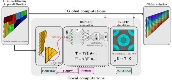
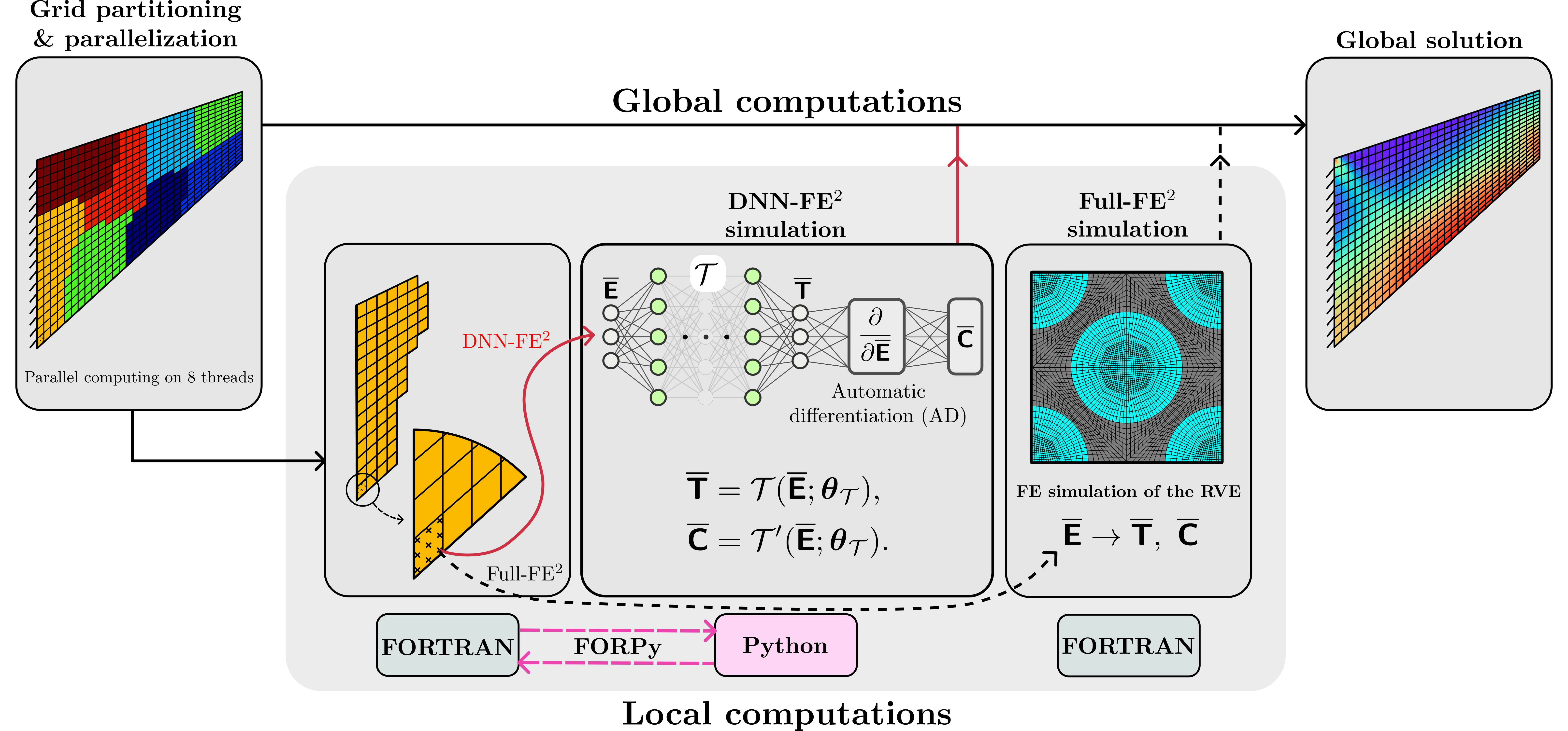
The main objective of the present work is to provide a consistent approach for employing deep neural networks (DNN) as surrogate models in step-size controlled multiscale FE${}^2$computations. As mentioned afore, various publications already deal with embedding artificial neural networks into numerical simulations especially for accelerating computational costly multiscale simulations. A novelty of the present work is that we provide a clear description of the algorithmic structure, which is in general a Multilevel–Newton algorithm (MLNA) that simplifies to a Newton–Raphson algorithm when employing DNN surrogate models. Further, current publications leave out required information; for example, the ways in which the consistent tangent at macroscale integration points is obtained from the microscale information, meaning whether the computations are performed by automatic differentiation, neural network models, or by numerical differentiation. Concerning this objective, we start in Section 2 with an explanation of the underlying equations and the algorithmic structure in FE${}^2$computations, where we restrict ourselves to small strains and quasi-static problems. Afterwards, two different architectures of neural networks and specific considerations of physical knowledge during the training process are described. Since the amount of training data required to obtain sufficient accuracies in the neural network outputs is of particular interest, this is investigated as well while using regular training and Sobolev training. As another novel contribution, we develop a method for efficiently coupling the different programming codes of the trained neural network and the multiscale finite element code. There, the application of high-performance computing libraries and just-in-time compilation yields significantly higher speed up of the DNN-FE${}^2$approach in load-step size controlled computations compared to the results presented in the current literature. Furthermore, the DNN surrogate is even able to overcome load-step size limitations that are apparent in FE${}^2$ computations.

The notation in use is defined in the following manner: geometrical vectors are symbolized by $\overrightarrow{a}$ and second-order tensors $\mathbf{A}$ by bold-faced Roman letters. In addition, we introduce column vectors and matrices at the global finite element level symbolized by bold-type italic letters $\mathit{A}$ and column vectors and matrices on the local (element) level using bold-type Roman letters $\mathbf{A}$. Further, to distinguish quantities on macroscale and microscale levels, we indicate microscale quantities by $\check{\langle ·\rangle }$. Calligraphic letters $\mathcal{A}$ denote deep neural network surrogate models.

2. Classical FE${}^{\mathbf{2}}$ Computations

In this work, finite elements are employed to perform multiscale computations; see, for example, [4,7]. Hence, only the main equations are recapped, which are necessary to explain the algorithmic structure. In multiscale FE${}^2$computations, the macro- and microscale levels have to be distinguished regarding the spatial discretization. Here, we restrict ourselves to periodic displacement boundary conditions on the microscale and refer to [4] for other boundary conditions on the microscale. The computation of the system of non-linear equations resulting from the spatial discretization is explained for the Multilevel–Newton algorithm (MLNA), which is here a two-level Newton algorithm. Further, the connection is drawn to embedding deep neural network surrogate models as predictors for homogenized quantities from the microscale in the MLNA.

2.1. Spatial Discretization

In the present work, FE${}^2$analyses are performed in a quasi-static setting with the restriction to small strains. Thus, no configurations have to be distinguished and we have the symmetric stress tensor $\mathbf{T}(\overrightarrow{x},t)$ and strain tensor $\mathbf{E}(\overrightarrow{x},t)=1/2\left(grad\overrightarrow{u}(\overrightarrow{x},t)+{grad}^T\overrightarrow{u}(\overrightarrow{x},t)\right)$ at positions $\overrightarrow{x}$ and time t. $\overrightarrow{u}(\overrightarrow{x},t)$ represents the displacement vector. The local balance of linear momentum has to be fulfilled. Here, the weak form is employed, which is also known as the principle of virtual displacements:

$$\pi (t,\mathbf{T},\delta \overrightarrow{u}):={\int }_V\delta \mathbf{E}\left(\overrightarrow{x}\right)·\mathbf{T}(\overrightarrow{x},t)\mathrm{d}V-{\int }_V\delta \overrightarrow{u}\left(\overrightarrow{x}\right)·\rho \left(\overrightarrow{x}\right)\overrightarrow{k}\mathrm{d}V-{\int }_A\delta \overrightarrow{u}\left(\overrightarrow{x}\right)·\overrightarrow{t}(\overrightarrow{x},t)\mathrm{d}A=0,$$

(1)

where $\delta \overrightarrow{u}\left(\overrightarrow{x}\right)$ are virtual displacements that are arbitrary but vanish at positions where the displacements $\overrightarrow{u}(\overrightarrow{x},t)$ are prescribed. Similarly, $\delta \mathbf{E}\left(\overrightarrow{x}\right)=1/2\left(grad\delta \overrightarrow{u}\left(\overrightarrow{x}\right)+{grad}^T\delta \overrightarrow{u}\left(\overrightarrow{x}\right)\right)$ represent virtual strains. Moreover, $\overrightarrow{k}$ symbolizes the acceleration of gravity. V and A denote the volume and surface of the material body and $\overrightarrow{t}$ are surface tractions. To develop the arising equations of the spatial discretization for three-dimensional continua on both macro- and microscale levels, a consistent matrix notation is followed.

2.1.1. Macroscale

Due to the spatial discretization, volume V and surface A transist into approximations $\mathsf{\Omega }$ and $\mathsf{\Gamma }$. Further, $\mathbf{x}\in \mathsf{\Omega }$ denote coordinates. Following a Galerkin-based finite element formulation, the ansatz for the displacements and virtual displacements read

$$\begin{array}{cc}\hfill {\mathit{u}}^h(\mathbf{x},t)& =\sum _{j=1}^{n_{\mathrm{nodes}}}{N}_j\left(\mathbf{x}\right){\mathbf{u}}_j\left(t\right)=\mathit{N}\left(\mathbf{x}\right)\mathit{u}\left(t\right)+\overline{\mathit{N}}\left(\mathbf{x}\right)\overline{\mathit{u}}\left(t\right)\stackrel{\mathrm{in}ⓔ}{=}{\mathbf{N}}^e\left({\phi }^e\left(\mathbf{x}\right)\right){\mathbf{u}}^e\left(t\right),\hfill \end{array}$$

(2)

$$\begin{array}{cc}\hfill \delta {\mathit{u}}^h(\mathbf{x},t)& =\sum _{j=1}^{n_{\mathrm{nodes}}}{N}_j\left(\mathbf{x}\right)\delta {\mathbf{u}}_j=\mathit{N}\left(\mathbf{x}\right)\delta \mathit{u}\stackrel{\mathrm{in}ⓔ}{=}{\mathbf{N}}^e\left({\phi }^e\left(\mathbf{x}\right)\right)\delta {\mathbf{u}}^e.\hfill \end{array}$$

(3)

${\mathbf{u}}_j{\in \mathbb{R}}^3$ and $\delta {\mathbf{u}}_j{\in \mathbb{R}}^3$ denote the macroscopic nodal displacement and virtual nodal displacement vector at node j. The shape functions are denoted by $N_j\left(\mathbf{x}\right)$, while $n_{\mathrm{nodes}}$ corresponds to the number of nodes on a macroscale level. In Equations (2) and (3), it is tacitly assumed that the displacements and virtual displacements are partitioned into unknown and prescribed quantities, i.e., $\mathit{u}{\in \mathbb{R}}^{n_{\mathrm{u}}}$ are unknown macroscale nodal displacements and $\overline{\mathit{u}}{\in \mathbb{R}}^{n_{\mathrm{p}}}$ are known (or prescribed) nodal displacements. Analogously, the arbitrary virtual displacements are denoted by $\delta \mathit{u}{\in \mathbb{R}}^{n_{\mathrm{u}}}$. For the prescribed virtual displacements on the macroscale $\delta \overline{\mathit{u}}=0$, $\delta \overline{\mathit{u}}{\in \mathbb{R}}^{n_{\mathrm{p}}}$ holds by definition. Thus, the number of degrees of freedom is $n_{\mathrm{a}}=n_{\mathrm{u}}+n_{\mathrm{p}}$. Further, the transition to a formulation of the displacements on element level in Equations (2) and (3) yields the matrix of shape functions ${\mathbf{N}}^e{\in \mathbb{R}}^{3\times n_{\mathrm{u}}^e}$ within an element, the element nodal displacements ${\mathbf{u}}^e{\in \mathbb{R}}^{n_{\mathrm{u}}^e}$, and corresponding virtual element nodal displacements $\delta {\mathbf{u}}^e{\in \mathbb{R}}^{n_{\mathrm{u}}^e}$. Here, $n_{\mathrm{u}}^e$ is the number of element nodal degrees of freedom. $\xi ={\phi }^e\left(\mathbf{x}\right)={\chi }^{e-1}\left(\mathbf{x}\right)$ are the local coordinates in the element domain with the coordinate transformation $\mathbf{x}={\chi }^e\left(\xi \right)$. The assignment between global and element quantities can be formulated as

$${\mathbf{u}}^e\left(t\right)={\mathit{Z}}^e\mathit{u}\left(t\right)+{\overline{\mathit{Z}}}^e\overline{\mathit{u}}\left(t\right),\delta {\mathbf{u}}^e={\mathit{Z}}^e\delta \mathit{u}.$$

(4)

Here, ${\mathit{Z}}^e{\in \mathbb{R}}^{n_{\mathrm{u}}^e\times n_{\mathrm{u}}}$ and ${\overline{\mathit{Z}}}^e{\in \mathbb{R}}^{n_{\mathrm{u}}^e\times n_{\mathrm{p}}}$ are formally introduced incidence matrices (Boolean matrices) which are not programmed but used here for the explanation of the assembling procedure of all element contributions. They assign the global unknown and prescribed nodal displacements to element e. Regarding an explanation of an implementation of these matrices, we refer to [73].

Moreover, the resulting strains and virtual strains read

$$\begin{array}{cc}\hfill {\mathit{E}}^h(\mathbf{x},t)& =\mathit{B}\left(\mathbf{x}\right)\mathit{u}\left(t\right)+\overline{\mathit{B}}\left(\mathbf{x}\right)\overline{\mathit{u}}\left(t\right)\stackrel{\mathrm{in}ⓔ}{=}{\mathbf{B}}^e\left({\phi }^e\left(\mathbf{x}\right)\right){\mathbf{u}}^e\left(t\right)={\mathbf{B}}^e\left({\phi }^e\left(\mathbf{x}\right)\right)({\mathit{Z}}^e\mathit{u}\left(t\right)+{\overline{\mathit{Z}}}^e\overline{\mathit{u}}\left(t\right)),\hfill \end{array}$$

(5)

$$\begin{array}{cc}\hfill \delta {\mathit{E}}^h(\mathbf{x},t)& =\mathit{B}\left(\mathbf{x}\right)\delta \mathit{u}\stackrel{\mathrm{in}ⓔ}{=}{\mathbf{B}}^e\left({\phi }^e\left(\mathbf{x}\right)\right)\delta {\mathbf{u}}^e={\mathbf{B}}^e\left({\phi }^e\left(\mathbf{x}\right)\right){\mathit{Z}}^e\delta \mathit{u}.\hfill \end{array}$$

(6)

Again, a decomposition into known and unknown nodal displacements is employed. Since the strain tensor is symmetric, $\mathbf{E}={\mathbf{E}}^T$, the strains can be written in the Voigt notation, i.e., ${\mathit{E}}^h{\in \mathbb{R}}^6$ and $\delta {\mathit{E}}^h{\in \mathbb{R}}^6$. $\mathit{B}{\in \mathbb{R}}^{6\times n_{\mathrm{u}}}$ and $\overline{\mathit{B}}{\in \mathbb{R}}^{6\times n_{\mathrm{p}}}$ denote the global strain–displacement matrices on the macroscale level for unknown and prescribed degrees of freedom, respectively, whose mathematical representation is extremely difficult to specify. Thus, the element strain–displacement matrix ${\mathbf{B}}^e{\in \mathbb{R}}^{6\times n_{\mathrm{u}}^e}$ is chosen. Inserting Equations (3) and (6) into the principle of virtual displacements (1) and performing a decomposition of the discretized domain into elements yields the non-linear equations on macroscale

$$\mathit{g}(t,\mathit{T}\left(t\right)):=\sum _{e=1}^{n_{\mathrm{e}}}{\mathit{Z}}^{eT}\left(\sum _{j=1}^{n_{\mathrm{G}}^e}{w}_j\mathbf{B}{}^{e\left(j\right)T}\mathbf{T}{}^{e\left(j\right)}\left(t\right)det\mathbf{J}{}^{e\left(j\right)}\right)-\overline{\mathit{P}}\left(t\right)=0,$$

(7)

$\mathit{g}{\in \mathbb{R}}^{n_{\mathrm{u}}}$. $n_{\mathrm{G}}^e$ is the number of integration points in an element on the macroscale. Further, $w_j$ denotes the weighting factors of the spatial integration technique, where here the Gauss-integration is drawn on. Accordingly, ${\xi }_j$ symbolizes the local coordinates of the integration points. Notation ${\langle ·\rangle }^{e\left(j\right)}$ is used to abbreviate quantities of element e at the macroscale integration point j, e.g., ${\mathbf{B}}^{e\left(j\right)}:={\mathbf{B}}^e\left({\xi }_j\right)$ for the strain–displacement matrix at integration point ${\xi }_j$. Since the coordinates are transformed into a reference domain, ${\mathbf{J}}^{e\left(j\right)}=\partial {\chi }^e/\partial \xi {|}_{\xi ={\xi }_j}$ is the Jacobian of the coordinate transformation. Moreover, $\overline{\mathit{P}}\left(t\right)$, $\overline{\mathit{P}}{\in \mathbb{R}}^{n_{\mathrm{u}}}$ represents the equivalent nodal force vector comprising the volume and surface distributed loads:

$$\overline{\mathit{p}}\left(t\right):={\int }_{\mathsf{\Omega }}{\mathit{N}}^T\left(\mathbf{x}\right)\rho \left(\mathbf{x}\right)\mathbf{k}\mathrm{d}\mathsf{\Omega }+{\int }_{\mathsf{\Gamma }}{\mathit{N}}^T\left(\mathbf{x}\right)\mathbf{t}(\mathbf{x},t)\mathrm{d}\mathsf{\Gamma }.$$

(8)

In Equation (7), $\mathbf{T}{}^{e\left(j\right)}{\in \mathbb{R}}^6$ are the stresses at a specific integration point j on the macroscale written in the Voigt notation. Usually, these quantities are obtained from the evaluation of particular constitutive models. In contrast, in FE${}^2$computations, the stresses are computed by a particular homogenization scheme of the microstructure, which is explained in the following section. The macroscopical strains at each integration point read with Equation (4)${}_1$

$$\mathbf{E}{}^{e\left(j\right)}(t,\mathit{u}\left(t\right))=\mathbf{B}{}^{e\left(j\right)}{\mathbf{u}}^e=\mathbf{B}{}^{e\left(j\right)}\left({\mathit{Z}}^e\mathit{u}\left(t\right)+{\overline{\mathit{Z}}}^e\overline{\mathit{u}}\left(t\right)\right).$$

(9)

Unfortunately, the principle of virtual displacements does not allow the computation of reaction forces. However, since the macroscale reaction forces are of interest in FE${}^2$computations, we choose here the Lagrange multiplier method; see [74] and the literature cited therein. Thus, the geometric constraint equation

$${\mathit{C}}_{\mathit{c}}(t,\widehat{\mathit{u}}\left(t\right))=\widehat{\mathit{u}}\left(t\right)-\overline{\mathit{u}}\left(t\right)=0$$

(10)

is introduced, ${\mathit{C}}_c{\in \mathbb{R}}^{n_{\mathrm{p}}}$. The prescribed displacements $\overline{\mathit{u}}\left(t\right)$ should be identical to the degrees of freedom $\widehat{\mathit{u}}\left(t\right)$, $\widehat{\mathit{u}}{\in \mathbb{R}}^{n_{\mathrm{p}}}$, representing the degrees of freedom that are initially assumed to be unknown as well. To satisfy constraint Equation (10), the Lagrange multipliers $\mathit{\lambda }{\in \mathbb{R}}^{n_{\mathrm{p}}}$ are required, which can be interpreted as the negative nodal forces.

The combining of Equations (7) and (10) provides the full system of equations for the discretized weak form of the balance of linear momentum on the macroscale, ${\mathit{g}}_{\mathrm{a}}{\in \mathbb{R}}^{n_{\mathrm{a}}}$,

$${\mathit{g}}_{\mathrm{a}}(t,\mathit{\lambda }\left(t\right),\mathit{T}\left(t\right)):=\left\{\begin{array}{c}{\displaystyle \sum _{e=1}^{n_{\mathrm{e}}}{\mathit{Z}}^{eT}\left(\sum _{j=1}^{n_{\mathrm{G}}^e}{w}_j\mathbf{B}{}^{e\left(j\right)T}\mathbf{T}{}^{e\left(j\right)}\left(t\right)det\mathbf{J}{}^{e\left(j\right)}\right)-\overline{\mathit{p}}\left(t\right)}\\ {\displaystyle \sum _{e=1}^{n_{\mathrm{e}}}{\overline{\mathit{Z}}}^{eT}\left(\sum _{j=1}^{n_{\mathrm{G}}^e}{w}_j\mathbf{B}{}^{e\left(j\right)T}\mathbf{T}{}^{e\left(j\right)}\left(t\right)det\mathbf{J}{}^{e\left(j\right)}\right)-\mathit{\lambda }\left(t\right)}\end{array}\right\}=0.$$

(11)

Remark 1.

It is worth mentioning that the consideration of reaction forces with the Lagrange multiplier method is performed to obtain a consistent variational formulation. The principle of virtual displacements does not allow the computation of reaction forces since they provide no virtual work (remember that $\delta \overline{\mathbf{u}}=0$ holds). Thus, another variational principle is required, which is here the Lagrange multiplier method. It is important to state that the Lagrange multipliers do not extend the number of unknowns in the application here, since they can be computed in a post-processing step after the computation of the nodal displacements; see Equation (11)${}_2$. Then, the Lagrange multipliers can be interpreted as nodal reaction forces, while considering that, of course, the accuracy of the results depends on the chosen termination criteria for the displacements. As a result, the application of the Lagrange multiplier method bypasses the evaluation of nodal equilibrium to compute the reaction forces at prescribed displacement degrees of freedom. The interested reader is referred to [74] for a detailed description of the method, and further references.

2.1.2. Microscale

The arising equations from the spatial discretization need to be studied also for the microstructure, which represents the discretized microscale geometry in FE${}^2$computations and is usually denoted as representative volume element (RVE). In contrast to common finite element simulations, where a constitutive model is evaluated at each integration point, here, the microstructure has to be evaluated.

The discretized weak form of the local equilibrium equation on the microscale can be derived analogously to the macroscale and reads

$${\check{\mathit{g}}}_{\mathrm{a}}^{e\left(j\right)}(t,{\mathit{u}}_{\mathrm{a}}\left(t\right),{\check{\mathit{u}}}_{\mathrm{a}}^{e\left(j\right)}\left(t\right))=\sum _{\check{e}=1}^{{\check{n}}_{\mathrm{e}}^{e\left(j\right)}}\check{\mathit{Z}}{}_{\mathrm{a}}^{\check{e}T}\left(\sum _{\check{j}=1}^{{\check{n}}_{\mathrm{G}}^{\check{e}}}{\check{w}}_{\check{j}}{\check{\mathbf{B}}}^{\check{e}\left(\check{j}\right)T}{\check{\mathbf{T}}}^{\check{e}\left(\check{j}\right)}\left(t\right)det{\check{\mathbf{J}}}^{\check{e}\left(\check{j}\right)}\right)=0.$$

(12)

Some remarks should be made regarding the above equation. First, ${\check{\mathit{u}}}_{\mathrm{a}}^{e\left(j\right)}{\in \mathbb{R}}^{{\check{n}}_{\mathrm{a}}^{e\left(j\right)}}$ are all displacements in the RVE at integration point j of macroscale element e. ${\check{n}}_{\mathrm{a}}^{e\left(j\right)}$ denotes the number of displacement degrees of freedom on the microscale. It is assumed that all displacements are initially unknown in the RVE. ${\check{n}}_{\mathrm{e}}^{e\left(j\right)}$ defines the number of elements on the microscale, ${\check{n}}_{\mathrm{G}}^{\check{e}}$ symbolizes the number of microscale integration points per element, and ${\check{w}}_{\check{j}}$ are the weights of the spatial integration. Matrix $\check{\mathit{Z}}{}_{\mathrm{a}}^{\check{e}T}{\in \mathbb{R}}^{{\check{n}}_{\mathrm{u}}^{\check{e}}\times {\check{n}}_{\mathrm{a}}^{e\left(j\right)}}$ denotes formally the assembling procedure of all element contributions and comprises matrices ${\check{\mathit{Z}}}^{\check{e}}{\in \mathbb{R}}^{{\check{n}}_{\mathrm{u}}^{\check{e}}\times {\check{n}}_{\mathrm{u}}^{e\left(j\right)}}$ and ${\overline{\check{\mathit{Z}}}}^{\check{e}}{\in \mathbb{R}}^{{\check{n}}_{\mathrm{u}}^{\check{e}}\times {\check{n}}_{\mathrm{p}}^{e\left(j\right)}}$ for the unknown and prescribed displacement degrees of freedom in the RVE, ${\check{n}}_{\mathrm{u}}^{e\left(j\right)}$ and ${\check{n}}_{\mathrm{p}}^{e\left(j\right)}$, respectively, $\check{\mathit{Z}}{}_{\mathrm{a}}^{\check{e}T}=\left[{\check{\mathit{Z}}}^{\check{e}}{\overline{\check{\mathit{Z}}}}^{\check{e}}\right]$. The strain–displacement matrix on the microscale is defined by ${\check{\mathbf{B}}}^{\check{e}\left(\check{j}\right)}{\in \mathbb{R}}^{6\times {\check{n}}_{\mathrm{u}}^{\check{e}}}$. Similarly to the macroscale, ${\check{n}}_{\mathrm{a}}^{e\left(j\right)}={\check{n}}_{\mathrm{u}}^{e\left(j\right)}+{\check{n}}_{\mathrm{p}}^{e\left(j\right)}$ holds. Moreover, at the microscale level, there are no volume or surface distributed loads, i.e., $\overline{\check{\mathit{p}}}=0$.

In this work, we restrict ourselves to periodic displacement boundary conditions on so-called conform spatial discretizations. We refer to [4] for a detailed description of boundary conditions on the microscale and to [75] regarding periodic displacement boundary conditions on non-conform discretizations. The underlying idea of periodic displacement boundary conditions is that the displacements of nodes, which are positioned on different parts of the surface of the RVE, are coupled. This coupling can be treated as a linear multiple point constraint problem. Thus, we introduce the primary and secondary displacements, ${\check{\mathit{u}}}_{\mathrm{M}}^{e\left(j\right)}{\in \mathbb{R}}^{{\check{n}}_{\mathrm{M}}^{e\left(j\right)}}$ and ${\check{\mathit{u}}}_{\mathrm{S}}^{e\left(j\right)}{\in \mathbb{R}}^{{\check{n}}_{\mathrm{S}}^{e\left(j\right)}}$. Here, ${\check{n}}_{\mathrm{K}}^{e\left(j\right)}={\check{n}}_{\mathrm{M}}^{e\left(j\right)}={\check{n}}_{\mathrm{S}}^{e\left(j\right)}$ holds for the number of pair-wise coupled displacement degrees of freedom ${\check{n}}_{\mathrm{K}}^{e\left(j\right)}$ and ${\check{n}}_{\mathrm{p}}^{e\left(j\right)}={\check{n}}_{\mathrm{S}}^{e\left(j\right)}$ for the prescribed degrees of freedom. Since the periodic displacements are applied on the surface of the RVE, the internal (within the volume of the RVE) displacement degrees of freedom are defined as ${\check{\mathit{u}}}_{\mathrm{V}}^{e\left(j\right)}{\in \mathbb{R}}^{{\check{n}}_{\mathrm{V}}^{e\left(j\right)}}$, where ${\check{n}}_{\mathrm{u}}^{e\left(j\right)}={\check{n}}_{\mathrm{V}}^{e\left(j\right)}+{\check{n}}_{\mathrm{M}}^{e\left(j\right)}$ holds. Accordingly, the decomposition of the nodal displacement degrees of freedom and the discretized local equilibrium Equation (12) on the microscale

$${\check{\mathit{u}}}_{\mathrm{a}}^{e\left(j\right)}=\left\{\begin{array}{c}{\check{\mathit{u}}}_{\mathrm{V}}^{e\left(j\right)}\\ {\check{\mathit{u}}}_{\mathrm{M}}^{e\left(j\right)}\\ {\check{\mathit{u}}}_{\mathrm{S}}^{e\left(j\right)}\end{array}\right\},{\check{\mathit{g}}}_{\mathrm{a}}^{e\left(j\right)}(t,{\mathit{u}}_{\mathrm{a}},{\check{\mathit{u}}}_{\mathrm{a}}^{e\left(j\right)}\left(t\right))=\left\{\begin{array}{c}{\check{\mathit{g}}}_{\mathrm{V}}^{e\left(j\right)}(t,{\mathit{u}}_{\mathrm{a}},{\check{\mathit{u}}}_{\mathrm{V}}^{e\left(j\right)},{\check{\mathit{u}}}_{\mathrm{M}}^{e\left(j\right)})\\ {\check{\mathit{g}}}_{\mathrm{M}}^{e\left(j\right)}(t,{\mathit{u}}_{\mathrm{a}},{\check{\mathit{u}}}_{\mathrm{V}}^{e\left(j\right)},{\check{\mathit{u}}}_{\mathrm{M}}^{e\left(j\right)})\\ {\check{\mathit{g}}}_{\mathrm{S}}^{e\left(j\right)}(t,{\mathit{u}}_{\mathrm{a}},{\check{\mathit{u}}}_{\mathrm{V}}^{e\left(j\right)},{\check{\mathit{u}}}_{\mathrm{M}}^{e\left(j\right)})\end{array}\right\},$$

(13)

is obtained.

The connection between the macro- and the microscale is achieved with macroscale displacements ${\mathit{u}}_{\mathrm{a}}\left(t\right)$ and microscale displacements ${\check{\mathit{u}}}_{\mathrm{a}}^{e\left(j\right)}\left(t\right)$ by specifying constraint

$${\check{\mathit{C}}}_{\mathrm{c}}^{e\left(j\right)}({\check{\mathit{u}}}_{\mathrm{a}}^{e\left(j\right)}\left(t\right),{\mathit{u}}_{\mathrm{a}}\left(t\right))={\check{\mathit{A}}}_1^{e\left(j\right)}{\check{\mathit{u}}}_{\mathrm{a}}^{e\left(j\right)}\left(t\right)-{\check{\mathit{A}}}_2^{e\left(j\right)}{\mathbf{E}}^{e\left(j\right)}\left({\mathit{u}}_{\mathrm{a}}\left(t\right)\right)=0,$$

(14)

with ${\check{\mathit{C}}}_{\mathrm{c}}^{e\left(j\right)}{\in \mathbb{R}}^{{\check{n}}_{\mathrm{p}}^{e\left(j\right)}}$, ${\check{\mathit{A}}}_1^{e\left(j\right)}{\in \mathbb{R}}^{{\check{n}}_{\mathrm{K}}^{e\left(j\right)}\times {\check{n}}_{\mathrm{a}}^{e\left(j\right)}}$, and ${\check{\mathit{A}}}_2^{e\left(j\right)}{\in \mathbb{R}}^{{\check{n}}_{\mathrm{K}}^{e\left(j\right)}\times 6}$. For the case of periodic displacement boundary conditions, matrices ${\check{\mathit{A}}}_1^{e\left(j\right)}$ and ${\check{\mathit{A}}}_2^{e\left(j\right)}$ read

$${\check{\mathit{A}}}_1^{e\left(j\right)}=\left[\underset{({\check{n}}_{\mathrm{K}}^{e\left(j\right)}\times {\check{n}}_{\mathrm{u}}^{e\left(j\right)})}{0_{\phantom{{}_{\mathrm{M}}}}}\underset{({\check{n}}_{\mathrm{M}}^{e\left(j\right)}\times {\check{n}}_{\mathrm{M}}^{e\left(j\right)})}{\check{\mathit{H}}{}_{\mathrm{M}}^{e\left(j\right)}}\underset{({\check{n}}_{\mathrm{S}}^{e\left(j\right)}\times {\check{n}}_{\mathrm{S}}^{e\left(j\right)})}{\check{\mathit{H}}{}_{\mathrm{S}}^{e\left(j\right)}}\right]\mathrm{and}{\check{\mathit{A}}}_2^{e\left(j\right)}=\check{\mathit{P}}{}^{e\left(j\right)T},$$

(15)

where matrices $\check{\mathit{H}}{}_{\mathrm{M}}^{e\left(j\right)}$ and $\check{\mathit{H}}{}_{\mathrm{S}}^{e\left(j\right)}$ are link-topology matrices that only contain the numbers 0, $+1$, $-1$. $\check{\mathit{P}}{}^{e\left(j\right)}{\in \mathbb{R}}^{6\times {\check{n}}_{\mathrm{K}}^{e\left(j\right)}}$ is a matrix that comprises the differences in the corresponding nodal positions. Constraint  (14) can be reformulated with $\check{\mathit{M}}{}^{e\left(j\right)}=\check{\mathit{H}}{}_{\mathrm{S}}^{e\left(j\right)-1}\check{\mathit{H}}{}_{\mathrm{M}}^{e\left(j\right)}$, $\check{\mathit{M}}{}^{e\left(j\right)}{\in \mathbb{R}}^{{\check{n}}_{\mathrm{S}}^{e\left(j\right)}\times {\check{n}}_{\mathrm{M}}^{e\left(j\right)}}$ leading to

$${\check{\mathit{C}}}_{\mathrm{c}}^{e\left(j\right)}({\check{\mathit{u}}}_{\mathrm{a}}^{e\left(j\right)}\left(t\right),{\mathit{u}}_{\mathrm{a}}\left(t\right))=\check{\mathit{M}}{}^{e\left(j\right)}{\check{\mathit{u}}}_{\mathrm{M}}^{e\left(j\right)}+{\check{\mathit{u}}}_{\mathrm{S}}^{e\left(j\right)}-\check{\mathit{H}}{}_{\mathrm{S}}^{e\left(j\right)-1}\check{\mathit{P}}{}^{e\left(j\right)T}{\mathbf{E}}^{e\left(j\right)}(t,\mathit{u}\left(t\right)).$$

(16)

Constraint (16) is, again, enforced with the microscale Lagrange multipliers ${\check{\mathit{\lambda }}}^{e\left(j\right)}{\in \mathbb{R}}^{{\check{n}}_{\mathrm{K}}^{e\left(j\right)}}$. With decomposition (13), the microscale strain vector ${\check{\mathbf{E}}}^{\check{e}\left(\check{j}\right)}{\in \mathbb{R}}^6$ of microscale element $\check{e}$ and integration point $\check{j}$ in dependence of the macroscale strains (9) reads

$${\check{\mathbf{E}}}^{\check{e}\left(\check{j}\right)}(t,\mathit{u},{\check{\mathit{u}}}^{e\left(j\right)})={\check{\mathbf{B}}}^{\check{e}\left(\check{j}\right)}\left\{{\check{\mathit{Z}}}^{\check{e}}{\check{\mathit{u}}}^{e\left(j\right)}+{\check{\mathit{Z}}}_{\mathrm{S}}^{\check{e}}\check{\mathit{H}}{}_{\mathrm{S}}^{e\left(j\right)-1}\check{\mathit{P}}{}^{e\left(j\right)T}{\mathbf{E}}^{e\left(j\right)}(t,\mathit{u}\left(t\right))\right\},$$

(17)

where we abbreviate

$${\check{\mathit{u}}}^{e\left(j\right)}=\left\{\begin{array}{c}{\check{\mathit{u}}}_{\mathrm{V}}^{e\left(j\right)}\\ {\check{\mathit{u}}}_{\mathrm{M}}^{e\left(j\right)}\end{array}\right\}{\check{\mathit{Z}}}^{\check{e}}=\left[{\check{\mathit{Z}}}_{\mathrm{V}}^{\check{e}}{\check{\mathit{Z}}}_{\mathrm{M}}^{\check{e}}-{\check{\mathit{Z}}}_{\mathrm{S}}^{\check{e}}\check{\mathit{M}}{}^{e\left(j\right)}\right].$$

(18)

${\check{\mathit{u}}}^{e\left(j\right)}{\in \mathbb{R}}^{{\check{n}}_{\mathrm{u}}^{e\left(j\right)}}$ denotes the assembled displacement vector, while ${\check{\mathit{Z}}}^{\check{e}}{\in \mathbb{R}}^{{\check{n}}_{\mathrm{u}}^{\check{e}}\times {\check{n}}_{\mathrm{u}}^{e\left(j\right)}}$, ${\check{\mathit{Z}}}_{\mathrm{V}}^{\check{e}}{\in \mathbb{R}}^{{\check{n}}_{\mathrm{u}}^{\check{e}}\times {\check{n}}_{\mathrm{V}}^{e\left(j\right)}}$, ${\check{\mathit{Z}}}_{\mathrm{M}}^{\check{e}}{\in \mathbb{R}}^{{\check{n}}_{\mathrm{u}}^{\check{e}}\times {\check{n}}_{\mathrm{M}}^{e\left(j\right)}}$, and ${\check{\mathit{Z}}}_{\mathrm{S}}^{\check{e}}{\in \mathbb{R}}^{{\check{n}}_{\mathrm{u}}^{\check{e}}\times {\check{n}}_{\mathrm{S}}^{e\left(j\right)}}$ represent assignment matrices.

In contrast to the macroscale, on the microscale, constitutive models are applied to describe the mechanical behavior of the materials. Since in this contribution, only elastic materials are studied, the constitutive model has the general form of

$${\check{\mathbf{T}}}^{\check{e}\left(\check{j}\right)}={\check{\mathbf{h}}}^{\check{e}\left(\check{j}\right)}\left({\check{\mathbf{E}}}^{\check{e}\left(\check{j}\right)}\right),$$

(19)

i.e., the evaluation of algebraic equations yields the stresses ${\check{\mathbf{T}}}^{\check{e}\left(\check{j}\right)}{\in \mathbb{R}}^6$ at the microscale integration points, which are already contained in Equation (12). What remains is the question of how to determine the required macroscale stress $\mathbf{T}{}^{e\left(j\right)}$ from the microscale evaluation. Here, a homogenization procedure is applied that fits into the general form of

$$\mathbf{T}{}^{e\left(j\right)}=\tilde{\mathbf{h}}{}^{e\left(j\right)}\left(\check{\mathit{\lambda }}{}^{e\left(j\right)}\left(t\right)\right)=\frac{1}{{\displaystyle \check{V}{}^{e\left(j\right)}}}{\check{\mathbf{A}}}_2{}^{e\left(j\right)T}\check{\mathit{\lambda }}{}^{e\left(j\right)}\left(t\right).$$

(20)

In the case of periodic displacement boundary conditions, the secondary displacements ${\check{\mathit{u}}}_{\mathrm{S}}^{e\left(j\right)}$ can be expressed by constraint (16)

$${\check{\mathit{u}}}_{\mathrm{S}}^{e\left(j\right)}=\check{\mathit{H}}{}_{\mathrm{S}}^{e\left(j\right)-1}\check{\mathit{P}}{}^{e\left(j\right)T}{\mathbf{E}}^{e\left(j\right)}(t,\mathit{u}\left(t\right))-\check{\mathit{M}}{}^{e\left(j\right)}{\check{\mathit{u}}}_{\mathrm{M}}^{e\left(j\right)}.$$

(21)

Further, enforcing constraint (16) yields, on the RVE level,

$${\check{\mathit{g}}}_{\mathrm{S}}^{e\left(j\right)}(t,{\mathit{u}}_{\mathrm{a}},{\check{\mathit{u}}}_{\mathrm{V}}^{e\left(j\right)},{\check{\mathit{u}}}_{\mathrm{M}}^{e\left(j\right)})-\check{\mathit{H}}{}_{\mathrm{S}}^{e\left(j\right)T}{\check{\mathit{\lambda }}}^{e\left(j\right)}=0.$$

(22)

This allows computation of microscale Lagrange multipliers ${\check{\mathit{\lambda }}}^{e\left(j\right)}$:

$${\check{\mathit{\lambda }}}^{e\left(j\right)}=\check{\mathit{H}}{}_{\mathrm{S}}^{e\left(j\right)-T}{\check{\mathit{g}}}_{\mathrm{S}}^{e\left(j\right)}(t,{\mathit{u}}_{\mathrm{a}},{\check{\mathit{u}}}_{\mathrm{V}}^{e\left(j\right)},{\check{\mathit{u}}}_{\mathrm{M}}^{e\left(j\right)}).$$

(23)

As a result, the homogenized stresses (20) on macroscale element e and integration point j read for periodic displacement boundary conditions:

$$\tilde{\mathbf{h}}{}^{e\left(j\right)}(t,{\mathit{u}}_{\mathrm{a}},{\check{\mathit{u}}}_{\mathrm{V}}^{e\left(j\right)},{\check{\mathit{u}}}_{\mathrm{M}}^{e\left(j\right)})=\frac{1}{{\displaystyle \check{V}{}^{e\left(j\right)}}}\check{\mathit{P}}{}^{e\left(j\right)}\check{\mathit{H}}{}_{\mathrm{S}}^{e\left(j\right)-T}{\check{\mathit{g}}}_{\mathrm{S}}^{e\left(j\right)}(t,{\mathit{u}}_{\mathrm{a}},{\check{\mathit{u}}}_{\mathrm{V}}^{e\left(j\right)},{\check{\mathit{u}}}_{\mathrm{M}}^{e\left(j\right)}).$$

(24)

2.1.3. General System of Non-Linear Equations

The entire system of equations of FE${}^2$computations with non-linear elastic material at the microscale level is obtained by formally assembling all independent variables of the RVEs:

$${\check{\mathit{u}}}_{\mathrm{a}}=\sum _{e=1}^{n_{\mathrm{e}}}\sum _{j=1}^{n_{\mathrm{G}}^e}{\mathit{Z}}_{{\check{\mathit{u}}}_{\mathrm{a}}}^{e\left(j\right)T}{\check{\mathit{u}}}_{\mathrm{a}}^{e\left(j\right)},\check{\mathit{\lambda }}=\sum _{e=1}^{n_{\mathrm{e}}}\sum _{j=1}^{n_{\mathrm{G}}^e}{\mathit{Z}}_{\check{\mathit{\lambda }}}^{e\left(j\right)T}{\check{\mathit{\lambda }}}^{e\left(j\right)},$$

(25)

${\check{\mathit{u}}}_{\mathrm{a}}{\in \mathbb{R}}^{n_{\mathrm{e}}{n}_{\mathrm{G}}^e{\check{n}}_{\mathrm{a}}^{e\left(j\right)}}$, $\check{\mathit{\lambda }}{\in \mathbb{R}}^{n_{\mathrm{e}}{n}_{\mathrm{G}}^e{\check{n}}_{\mathrm{K}}^{e\left(j\right)}}$, as well as equations

$$\begin{array}{cc}\hfill {\check{\mathit{g}}}_{\mathrm{a}}({\check{\mathit{u}}}_{\mathrm{a}},\check{\mathit{\lambda }})& =\sum _{e=1}^{n_{\mathrm{e}}}\sum _{j=1}^{n_{\mathrm{G}}^e}{\mathit{Z}}_{{\check{\mathit{u}}}_{\mathrm{a}}}^{e\left(j\right)T}\left\{{\check{\mathit{g}}}_{\mathrm{a}}^{e\left(j\right)}\left({\check{\mathit{u}}}_{\mathrm{a}}^{e\left(j\right)}\right)-{\check{\mathit{A}}}_1^{e\left(j\right)T}{\check{\mathit{\lambda }}}^{e\left(j\right)}\right\},\hfill \end{array}$$

(26)

$$\begin{array}{cc}\hfill {\check{\mathit{C}}}_{\mathrm{c}}({\mathit{u}}_{\mathrm{a}},{\check{\mathit{u}}}_{\mathrm{a}})& =\sum _{e=1}^{n_{\mathit{e}}}\sum _{j=1}^{n_{\mathrm{G}}^e}{\mathit{Z}}_{\check{\mathit{\lambda }}}^{e\left(j\right)T}{\check{\mathit{C}}}_{\mathrm{c}}^{e\left(j\right)}({\mathit{u}}_{\mathrm{a}},{\check{\mathit{u}}}_{\mathrm{a}}^{e\left(j\right)}).\hfill \end{array}$$

(27)

The entire system of non-linear equations is obtained by compiling macroscale Equations (10) and (11) and microscale Equations (26) and (27). The number of equations can be essentially reduced by assuming that constraint (10) is fulfilled after solving the entire system of non-linear equations and by employing Equation (23) on the microscale for periodic displacement boundary conditions. Further, ${\check{\mathit{A}}}_1^{e\left(j\right)}$, as given in Equation (15)${}_1$, can be applied. Then, the reduced system of non-linear equations,

$$\mathit{F}(t,\mathit{y})=\left\{\begin{array}{c}\mathit{g}(t,\mathit{u})\\ {\check{\mathit{g}}}_{\mathrm{V}}(t,\mathit{u},{\check{\mathit{u}}}_{\mathrm{V}},{\check{\mathit{u}}}_{\mathrm{M}})\\ {\check{\mathit{g}}}_{\mathrm{M}}(t,\mathit{u},{\check{\mathit{u}}}_{\mathrm{V}},{\check{\mathit{u}}}_{\mathrm{M}})-{\check{\mathit{M}}}^T{\check{\mathit{g}}}_{\mathrm{S}}(t,\mathit{u},{\check{\mathit{u}}}_{\mathrm{V}},{\check{\mathit{u}}}_{\mathrm{M}})\end{array}\right\}=0,$$

(28)

which is the result of the spatial discretization, has to be solved at each load-step (time-step) with the vector of unknowns

$${\mathit{y}}^T={\{\mathit{u},{\check{\mathit{u}}}_{\mathrm{V}},{\check{\mathit{u}}}_{\mathrm{M}}\}}^T.$$

(29)

In the equations mentioned above, ${\check{\mathit{u}}}_{\mathrm{V}}$ and ${\check{\mathit{u}}}_{\mathrm{M}}$ are the vectors of assembled internal microscale nodal displacements ${\check{\mathit{u}}}_{\mathrm{V}}^{e\left(j\right)}$ and primary nodal displacements ${\check{\mathit{u}}}_{\mathrm{M}}^{e\left(j\right)}$, respectively.

Remark 2.

Further, an important aspect is the time discretization. Since only non-linear elastic material is studied here, Equation (28) represents a purely algebraic system of equations. Nevertheless, time integration methods, such as the Backward–Euler method, can be applied when formally extending Equation (28) with $\dot{t}=1$ to obtain a system of differential-algebraic equations (DAE), as it is common in finite element computations, where the inelastic material behavior is described by evolution equations for some internal variables [76]. As a result, the application of time integration methods to elastic problems leads to an incremental application of the prescribed loads, which is therefore achieved in the numerical examples of this work. In the case of non-linear elastic material behavior, the load is often applied step-wise, where the previous solution of the nodal displacements is inserted into some Newton-like scheme as starting vector to be close to the solution. Otherwise, problems in the convergence of the iterative scheme are observed. In this sense, the step-wise increase in the load (displacement- or force-controlled) can be interpreted as time integration.

2.2. Multilevel–Newton Algorithm

What remains is the question of how the system of non-linear Equation (28) is solved in multiscale simulations. Further, to sufficiently embed DNN surrogates, it is important to make clear which parts of the overall computation scheme can be substituted with minimal changes in a finite element program, as it is discussed later on.

There are different approaches to solve the system of non-linear Equation (28). First, the entire system of equations could be solved with the Newton–Raphson method, but this would only be possible for smaller problems due to the extremely large number of equations. An alternative—see [76]—would be to use the Newton–Schur complement, which, on the one hand, requires some intervention in the coding and provision of the derivatives [77]. In traditional approaches, on the other hand, one uses the MLNA considering periodic boundary conditions for the microstructures. Therefore, in order to see what advantage neural networks have here, the Multilevel–Newton algorithm (MLNA) approach is briefly explained.

Since the MLNA, which was originally introduced by [78,79], is frequently applied, we refer especially to [76] regarding the differences between the MLNA and the well-known Newton–Raphson scheme. Thus, only the required equations are recapped here to show the general algorithmic structure of FE${}^2$computations and the incorporation of DNN surrogate models.

If we interpret the incremental load-control as time integration, the non-linear system (28) has to be evaluated at time $t_{n+1}$, $t_{n+1}=t_n+\Delta t_n$. Thus, in each time-step, the unknown microscale displacements $\check{\mathit{u}}={\{{\check{\mathit{u}}}_{\mathrm{V}},{\check{\mathit{u}}}_{\mathrm{M}}\}}^T$, see Equation (18)${}_1$, and the unknown macroscale displacements $\mathit{u}$ are sought. For further treatment of the equations, we also introduce decomposition

$$\check{\mathit{G}}\widehat{=}\left\{\begin{array}{c}{\check{\mathit{g}}}_{\mathrm{V}}\\ {\check{\mathit{g}}}_{\mathrm{M}}-{\check{\mathit{M}}}^T{\check{\mathit{g}}}_{\mathrm{S}}\end{array}\right\}.$$

(30)

Thus, the system of non-linear equations

$$\begin{array}{cc}\hfill \mathit{G}(\mathit{u},\check{\mathit{u}})& =0,\hfill \\ \hfill \check{\mathit{G}}(\mathit{u},\check{\mathit{u}})& =0\hfill \end{array}$$

(31)

has to be solved.

2.2.1. Multilevel–Newton Algorithm for FE${}^2$ Computations

In the traditional manner, the MLNA is applied to solve Equation (31). The scheme draws on the implicit function theorem, i.e., it is assumed that function $\check{\mathit{u}}=\widehat{\check{\mathit{u}}}\left(\mathit{u}\right)$ exists. In other words,

$$\mathit{G}(\mathit{u},\widehat{\check{\mathit{u}}}\left(\mathit{u}\right))=0$$

(32)

has to be solved. The Newton–Raphson method applied to the non-linear system (32) requires in each iteration step the computation of linear system

$$\left[\frac{{\displaystyle \partial \mathit{G}}}{{\displaystyle \partial \mathit{u}}}+\frac{{\displaystyle \partial \mathit{G}}}{{\displaystyle \partial \check{\mathit{u}}}}\frac{{\displaystyle \mathrm{d}\widehat{\check{\mathit{u}}}}}{{\displaystyle \mathrm{d}\mathit{u}}}\right]\Delta \mathit{u}=-\mathit{G}(\mathit{u},\widehat{\check{\mathit{u}}}\left(\mathit{u}\right)).$$

(33)

Here, the iteration index is omitted for brevity. Quantities $\mathrm{d}\widehat{\check{\mathit{u}}}/\mathrm{d}\mathit{u}$ and $\check{\mathit{u}}=\widehat{\check{\mathit{u}}}\left(\mathit{u}\right)$ have to be provided by two additional computational steps, since $\widehat{\check{\mathit{u}}}\left(\mathit{u}\right)$ is assumed to exist, but its representation is unknown. First,

$$\check{\mathit{G}}(\mathit{u},\check{\mathit{u}})=0⇝\check{\mathit{u}}$$

(34)

is evaluated for a given $\mathit{u}$, and second, the chain-rule is applied to

$$\check{\mathit{G}}(\mathit{u},\widehat{\check{\mathit{u}}}\left(\mathit{u}\right))=0\to \frac{{\displaystyle \partial \check{\mathit{G}}}}{{\displaystyle \partial \mathit{u}}}+\frac{{\displaystyle \partial \check{\mathit{G}}}}{{\displaystyle \partial \check{\mathit{u}}}}\frac{{\displaystyle \mathrm{d}\widehat{\check{\mathit{u}}}}}{{\displaystyle \mathrm{d}\mathit{u}}}=0⇝\frac{{\displaystyle \mathrm{d}\widehat{\check{\mathit{u}}}}}{{\displaystyle \mathrm{d}\mathit{u}}}.$$

(35)

The entire procedure is shown in Algorithm 1.

In greater detail and with the problem at hand, we proceed as follows. On a microscale, the system of non-linear equations

$${\displaystyle \check{\mathit{G}}(t_{n+1},\mathit{u},{\check{\mathit{u}}}_{\mathrm{V}},{\check{\mathit{u}}}_{\mathrm{M}})=\sum _{e=1}^{n_{\mathrm{e}}}\sum _{j=1}^{n_{\mathit{G}}^e}{\mathit{Z}}_{\check{\mathit{u}}}^{e\left(j\right)T}{\check{\mathit{G}}}^{e\left(j\right)}(t_{n+1},\mathit{u},{\check{\mathit{u}}}_{\mathrm{V}}^{e\left(j\right)},{\check{\mathit{u}}}_{\mathrm{M}}^{e\left(j\right)})=0}$$

(36)

has to be be solved for the case of periodic displacement boundary conditions, with 

$${\check{\mathit{G}}}^{e\left(j\right)}(t_{n+1},\mathit{u},{\check{\mathit{u}}}_{\mathrm{V}}^{e\left(j\right)},{\check{\mathit{u}}}_{\mathrm{M}}^{e\left(j\right)})=\sum _{\check{e}=1}^{{\check{n}}_{\mathrm{e}}^{e\left(j\right)}}\check{\mathit{Z}}{}^{\check{e}T}\left(\sum _{\check{j}=1}^{{\check{n}}_{\mathit{G}}^{\check{e}}}{\check{w}}_{\check{j}}{\check{\mathbf{B}}}^{\check{e}\left(\check{j}\right)T}{\check{\mathbf{h}}}^{\check{e}\left(\check{j}\right)}\left({\check{\mathbf{E}}}^{\check{e}\left(\check{j}\right)}\right)det{\check{\mathbf{J}}}^{\check{e}\left(\check{j}\right)}\right).$$

(37)

Here, ${\check{\mathit{Z}}}^{\check{e}}$ still has representation (18)${}_2$, which then leads to the second and third equations of Equation (28). For purely elastic problems, the solution of Equation (36) leads to a linear system on global microscale level within the Newton-iteration step to solve Equation (34),

$$\left[\frac{{\displaystyle \partial \check{\mathit{G}}}}{{\displaystyle \partial \check{\mathit{u}}}}\right]\Delta \check{\mathit{u}}=-\check{\mathit{G}}(\mathit{u},\check{\mathit{u}}),$$

(38)

which reads, in detail, as

$${\left.\left[\begin{array}{cc}\frac{{\displaystyle \partial {\check{\mathit{G}}}_{\mathrm{V}}}}{{\displaystyle \partial {\check{\mathit{u}}}_{\mathrm{V}}}}& \frac{{\displaystyle \partial {\check{\mathit{G}}}_{\mathrm{V}}}}{{\displaystyle \partial {\check{\mathit{u}}}_{\mathrm{M}}}}\\ \frac{{\displaystyle \partial {\check{\mathit{G}}}_{\mathrm{M}}}}{{\displaystyle \partial {\check{\mathit{u}}}_{\mathrm{V}}}}-{\check{\mathit{M}}}^T\left[\frac{{\displaystyle \partial {\check{\mathit{G}}}_{\mathrm{S}}}}{{\displaystyle \partial {\check{\mathit{u}}}_{\mathrm{V}}}}\right]& \frac{{\displaystyle \partial {\check{\mathit{G}}}_{\mathrm{M}}}}{{\displaystyle \partial {\check{\mathit{u}}}_{\mathrm{M}}}}-{\check{\mathit{M}}}^T\left[\frac{{\displaystyle \partial {\check{\mathit{G}}}_{\mathrm{S}}}}{{\displaystyle \partial {\check{\mathit{u}}}_{\mathrm{M}}}}\right]\end{array}\right]\right|}_{\mathit{y}}\left\{\begin{array}{c}{\displaystyle \Delta {\check{\mathit{u}}}_{\mathrm{V}}}\\ {\displaystyle \Delta {\check{\mathit{u}}}_{\mathrm{M}}}\end{array}\right\}=-\left\{\begin{array}{c}{\displaystyle {\check{\mathit{G}}}_{\mathrm{V}}\left(\mathit{y}\right)}\\ {\displaystyle {\check{\mathit{G}}}_{\mathrm{M}}\left(\mathit{y}\right)-{\check{\mathit{M}}}^T{\check{\mathit{G}}}_{\mathrm{S}}\left(\mathit{y}\right)}\end{array}\right\}$$

(39)

with the vector of unknowns $\mathit{y}$ according to Equation (29)${}_1$. We apply another relationship between microscale displacements ${\check{\mathit{u}}}^{e\left(j\right)}$ and the assembled microscale displacements $\check{\mathit{u}}$, ${\check{\mathit{u}}}^{e\left(j\right)}={\mathit{Z}}_{\check{\mathit{u}}}^{e\left(j\right)}\check{\mathit{u}}$. The system of linear Equation (38) can be re-written employing the chain rule and applying the decomposition into the macroscale integration point contributions, i.e., contributions of each RVE,

$${\displaystyle \sum _{e=1}^{n_{\mathrm{e}}}\sum _{j=1}^{n_{\mathrm{G}}^e}{\mathit{Z}}_{\check{\mathit{u}}}^{e\left(j\right)T}\left\{\left[\frac{{\displaystyle \partial {\check{\mathit{G}}}^{e\left(j\right)}}}{{\displaystyle \partial {\check{\mathit{u}}}^{e\left(j\right)}}}\right]\Delta {\check{\mathit{u}}}^{e\left(j\right)}+{\check{\mathit{G}}}^{e\left(j\right)}(\mathit{u},{\check{\mathit{u}}}^{e\left(j\right)})\right\}=0.}$$

(40)

Algorithm 1: Multilevel-Newton algorithm for FE2 computations with periodic displacement boundary conditions on a microscale.

For abbreviation purposes, we introduce the global microscale tangential stiffness matrix

$${\check{\mathit{K}}}^{e\left(j\right)}:=\frac{{\displaystyle \partial {\check{\mathit{G}}}^{e\left(j\right)}}}{{\displaystyle \partial {\check{\mathit{u}}}^{e\left(j\right)}}}=\frac{{\displaystyle \partial {\check{\mathit{G}}}^{e\left(j\right)}}}{{\displaystyle \partial {\check{\mathbf{E}}}^{\check{e}\left(\check{j}\right)}}}\frac{{\displaystyle \mathrm{d}{\widehat{\check{\mathbf{E}}}}^{\check{e}\left(\check{j}\right)}}}{{\displaystyle \mathrm{d}{\check{\mathit{u}}}^{e\left(j\right)}}},$$

(41)

${\check{\mathit{K}}}^{e\left(j\right)}{\in \mathbb{R}}^{{\check{n}}_{\mathrm{u}}^{e\left(j\right)}\times {\check{n}}_{\mathrm{u}}^{e\left(j\right)}}$. Using Equations (17) and (37),

$${\check{\mathit{K}}}^{e\left(j\right)}=\sum _{\check{e}=1}^{{\check{n}}_{\mathrm{e}}^{e\left(j\right)}}\check{\mathit{Z}}{}^{\check{e}T}\underset{\check{\mathbf{k}}{}^{\check{e}}}{\underbrace{\left[\sum _{\check{j}=1}^{{\check{n}}_{\mathit{G}}^{\check{e}}}{\check{w}}_{\check{j}}{\check{\mathbf{B}}}^{\check{e}\left(\check{j}\right)T}\underset{{\check{\mathbf{C}}}^{\check{e}\left(\check{j}\right)}}{\underbrace{\left[\frac{{\displaystyle \partial {\check{\mathbf{h}}}^{\check{e}\left(\check{j}\right)}}}{{\displaystyle \partial {\check{\mathbf{E}}}^{\check{e}\left(\check{j}\right)}}}\right]}}{\check{\mathbf{B}}}^{\check{e}\left(\check{j}\right)}det{\check{\mathbf{J}}}^{\check{e}\left(\check{j}\right)}\right]}}{\check{\mathit{Z}}}^{\check{e}}$$

(42)

is obtained, where ${\check{\mathbf{C}}}^{\check{e}\left(\check{j}\right)}{\in \mathbb{R}}^{6\times 6}$ denotes the consistent tangent matrix at microscale integration point $\check{j}$ of element $\check{e}$, and $\check{\mathbf{k}}{}^{\check{e}}{\in \mathbb{R}}^{{\check{n}}_{\check{\mathrm{u}}}^{\check{e}}\times {\check{n}}_{\check{\mathrm{u}}}^{\check{e}}}$ defines the element stiffness matrix of an element in an RVE. As a result, on a microscale, i.e., each RVE, the system of linear equations

$${\check{\mathit{K}}}^{e\left(j\right)}\Delta {\check{\mathit{u}}}^{e\left(j\right)}=-{\check{\mathit{G}}}^{e\left(j\right)}(\mathit{u},{\check{\mathit{u}}}^{e\left(j\right)})$$

(43)

has to be sequentially solved on a global microscale level to reach microscale equilibrium. In other words, the solution of system (43) is repeated until a local convergence criterion is fulfilled. Then, the microscale displacements $\check{\mathit{u}}$ are obtained.

As the next step, the macroscale consistent linearization (35) implies

$$\frac{{\displaystyle \partial \check{\mathit{G}}}}{{\displaystyle \partial \check{\mathit{u}}}}\frac{{\displaystyle \mathrm{d}\widehat{\check{\mathit{u}}}}}{{\displaystyle \mathrm{d}\mathit{u}}}=-\frac{{\displaystyle \partial \check{\mathit{G}}}}{{\displaystyle \partial \mathit{u}}}.$$

(44)

These matrices read under consideration of Equations (9), (17) and (42):

$$\begin{array}{cc}\hfill \frac{{\displaystyle \partial \check{\mathit{G}}}}{{\displaystyle \partial \check{\mathit{u}}}}\frac{{\displaystyle \mathrm{d}\widehat{\check{\mathit{u}}}}}{{\displaystyle \mathrm{d}\mathit{u}}}& {\displaystyle =\sum _{e=1}^{n_{\mathrm{e}}}\sum _{j=1}^{n_{\mathrm{G}}^e}{\mathit{Z}}_{\check{\mathit{u}}}^{e\left(j\right)T}\left[\sum _{\check{e}=1}^{{\check{n}}_{\mathrm{e}}^{e\left(j\right)}}\check{\mathit{Z}}{}^{\check{e}T}\check{\mathbf{k}}{}^{\check{e}}{\check{\mathit{Z}}}^{\check{e}}\right]\frac{{\displaystyle \mathrm{d}{\check{\mathit{u}}}^{e\left(j\right)}}}{{\displaystyle \mathrm{d}\mathbf{E}{}^{e\left(j\right)}}}\underset{\mathbf{B}{}^{e\left(j\right)}{\mathit{Z}}^e}{\underbrace{\frac{{\displaystyle \mathrm{d}\widehat{\mathbf{E}}{}^{e\left(j\right)}}}{{\displaystyle \mathrm{d}\mathit{u}}}}},}\hfill \end{array}$$

(45)

$$\begin{array}{cc}\hfill \frac{{\displaystyle \partial \check{\mathit{G}}}}{{\displaystyle \partial \mathit{u}}}& {\displaystyle =\sum _{e=1}^{n_{\mathrm{e}}}\sum _{j=1}^{n_{\mathrm{G}}^e}{\mathit{Z}}_{\check{\mathit{u}}}^{e\left(j\right)T}\left[\sum _{\check{e}=1}^{{\check{n}}_{\mathrm{e}}^{e\left(j\right)}}\check{\mathit{Z}}{}^{\check{e}T}\check{\mathbf{k}}{}^{\check{e}}{\check{\mathit{Z}}}_{\mathrm{S}}^{\check{e}}\right]\check{\mathit{H}}{}_{\mathrm{S}}^{e\left(j\right)-1}\check{\mathit{P}}{}^{e\left(j\right)T}\frac{{\displaystyle \mathrm{d}\widehat{\mathbf{E}}{}^{e\left(j\right)}}}{{\displaystyle \mathrm{d}\mathit{u}}},}\hfill \end{array}$$

(46)

where $\partial {\check{\mathbf{E}}}^{\check{e}\left(\check{j}\right)}/\partial \mathbf{E}{}^{e\left(j\right)}={\check{\mathbf{B}}}^{\check{e}\left(\check{j}\right)}{\check{\mathit{Z}}}_{\mathrm{S}}^{\check{e}}\check{\mathit{H}}{}_{\mathrm{S}}^{e\left(j\right)-1}\check{\mathit{P}}{}^{e\left(j\right)T}$ is used in Equation (46). Then, with the two matrices

$${\check{\mathit{K}}}^{e\left(j\right)}=\sum _{\check{e}=1}^{{\check{n}}_{\mathrm{e}}^{e\left(j\right)}}\check{\mathit{Z}}{}^{\check{e}T}\check{\mathbf{k}}{}^{\check{e}}{\check{\mathit{Z}}}^{\check{e}}\mathrm{and}{\overline{\check{\mathit{K}}}}^{e\left(j\right)}=\sum _{\check{e}=1}^{{\check{n}}_{\mathrm{e}}^{e\left(j\right)}}\check{\mathit{Z}}{}^{\check{e}T}\check{\mathbf{k}}{}^{\check{e}}{\check{\mathit{Z}}}_{\mathrm{S}}^{\check{e}},$$

(47)

${\overline{\check{\mathit{K}}}}^{e\left(j\right)}{\in \mathbb{R}}^{{\check{n}}_{\mathrm{u}}^{e\left(j\right)}\times {\check{n}}_{\mathrm{S}}^{e\left(j\right)}}$, on a global RVE level, the consistent linearization step (44) for each RVE reads

$${\check{\mathit{K}}}^{e\left(j\right)}\frac{{\displaystyle \mathrm{d}{\check{\mathit{u}}}^{e\left(j\right)}}}{{\displaystyle \mathrm{d}\mathbf{E}{}^{e\left(j\right)}}}=-{\overline{\check{\mathit{K}}}}^{e\left(j\right)}\check{\mathit{H}}{}_{\mathrm{S}}^{e\left(j\right)-1}\check{\mathit{P}}{}^{e\left(j\right)T}$$

(48)

in order to compute $\mathrm{d}{\check{\mathit{u}}}^{e\left(j\right)}/\mathrm{d}\mathbf{E}{}^{e\left(j\right)}$ and, finally, $\mathrm{d}\widehat{\stackrel{ˇ}{\mathit{u}}}/\mathrm{d}\mathit{u}$. Therewith, the local macroscale computations consisting of the two steps, the global microscale level and the macroscale consistent linearization, are finalized.

As a last step in the MLNA, the system of linear equations

$${\left.\left[\frac{{\displaystyle \partial \mathit{G}}}{{\displaystyle \partial \mathit{u}}}+\frac{{\displaystyle \partial \mathit{G}}}{{\displaystyle \partial \check{\mathit{u}}}}\frac{{\displaystyle \mathrm{d}\widehat{\stackrel{ˇ}{\mathit{u}}}}}{{\displaystyle \mathrm{d}\mathit{u}}}\right]\right|}_{\mathit{y}}\Delta \mathit{u}=-\mathrm{G}\left(\mathit{y}\right),\mathrm{with}\mathit{y}=\left\{\begin{array}{c}\mathit{u}\\ \check{\mathit{u}}\end{array}\right\},$$

(49)

see Equation (33), has to be solved at a global macroscale level to compute the increment $\Delta \mathit{u}$ of the macroscale displacements. Here, $\mathit{G}$ is the discretized weak formulation of the equilibrium equation at the macroscale; see Equation (7),

$$\mathit{G}(t_{n+1},\mathit{u},\check{\mathit{u}})=\sum _{e=1}^{n_{\mathrm{e}}}{\mathit{Z}}^{eT}\left(\sum _{j=1}^{n_{\mathrm{G}}^e}{w}_j\mathbf{B}{}^{e\left(j\right)T}\underset{\mathbf{T}{}^{e\left(j\right)}}{\underbrace{\tilde{\mathbf{h}}{}^{e\left(j\right)}(t_{n+1},\mathit{u},{\check{\mathit{u}}}^{e\left(j\right)})}}det\mathbf{J}{}^{e\left(j\right)}\right)-\overline{\mathit{p}}\left(t_{n+1}\right)=0,$$

(50)

in dependence of the homogenized stress state $\mathbf{T}{}^{e\left(j\right)}$ from Equation (20). Analogously to Equation (41), we define the global tangential stiffness matrix

$$\begin{array}{cc}\mathrm{K}\hfill & :=\frac{{\displaystyle \partial \mathit{G}}}{{\displaystyle \partial \mathit{u}}}+\frac{{\displaystyle \partial \mathit{G}}}{{\displaystyle \partial \check{\mathit{u}}}}\frac{{\displaystyle \mathrm{d}\widehat{\stackrel{ˇ}{\mathit{u}}}}}{{\displaystyle \mathrm{d}\mathit{u}}},\hfill \end{array}$$

(51)

$$\begin{array}{cc}\hfill & =\sum _{e=1}^{n_{\mathrm{e}}}{\mathit{Z}}^{eT}\left[\sum _{j=1}^{n_{\mathrm{G}}^e}{w}_j\mathbf{B}{}^{e\left(j\right)T}\frac{1}{{\displaystyle \check{V}{}^{e\left(j\right)}}}\check{\mathit{P}}{}^{e\left(j\right)}\check{\mathit{H}}{}_{\mathrm{S}}^{e\left(j\right)-T}\left[\frac{{\displaystyle \partial {\check{\mathit{G}}}_{\mathrm{S}}^{e\left(j\right)}}}{{\displaystyle \partial \mathit{u}}}+\frac{{\displaystyle \partial {\check{\mathit{G}}}_{\mathrm{S}}^{e\left(j\right)}}}{{\displaystyle \partial \check{\mathit{u}}}}\frac{{\displaystyle \mathrm{d}\widehat{\stackrel{ˇ}{\mathit{u}}}}}{{\displaystyle \mathrm{d}\mathit{u}}}\right]det\mathbf{J}{}^{e\left(j\right)}\right].\hfill \end{array}$$

(52)

$\mathit{K}{\in \mathbb{R}}^{n_{\mathrm{u}}\times n_{\mathrm{u}}}$, where Equation (20) is already employed in Equation (52). Again, the derivatives can be re-formulated applying the chain rule and the microscale element stiffness matrix $\check{\mathbf{k}}{}^{\check{e}}$ from Equation (42):

$$\begin{array}{cc}\hfill \frac{{\displaystyle \partial {\check{\mathit{G}}}_{\mathrm{S}}^{e\left(j\right)}}}{{\displaystyle \partial \mathit{u}}}& =\frac{{\displaystyle \partial {\check{\mathit{G}}}_{\mathrm{S}}^{e\left(j\right)}}}{{\displaystyle \partial {\check{\mathbf{E}}}^{\check{e}\left(\check{j}\right)}}}\frac{{\displaystyle \partial {\widehat{\stackrel{ˇ}{\mathbf{E}}}}^{\check{e}\left(\check{j}\right)}}}{{\displaystyle \partial \mathbf{E}{}^{e\left(j\right)}}}\frac{{\displaystyle \mathrm{d}\hat{\mathbf{E}}{}^{e\left(j\right)}}}{{\displaystyle \mathrm{d}\mathit{u}}}=\underset{{\overline{\overline{\check{\mathit{K}}}}}^{e\left(j\right)}}{\underbrace{\left[\sum _{\check{e}=1}^{{\check{n}}_{\mathrm{e}}^{e\left(j\right)}}\check{\mathit{Z}}{}_{\mathrm{S}}^{\check{e}T}\check{\mathbf{k}}{}^{\check{e}}{\check{\mathit{Z}}}_{\mathrm{S}}^{\check{e}}\right]}}\check{\mathit{H}}{}_{\mathrm{S}}^{e\left(j\right)-1}\check{\mathit{P}}{}^{e\left(j\right)T}\mathbf{B}{}^{e\left(j\right)}{\mathit{Z}}^e,\hfill \end{array}$$

(53)

$$\begin{array}{cc}\hfill \frac{{\displaystyle \partial {\check{\mathrm{G}}}_{\mathrm{S}}^{e\left(j\right)}}}{{\displaystyle \partial \check{\mathit{u}}}}\frac{{\displaystyle \mathrm{d}\widehat{\stackrel{ˇ}{\mathit{u}}}}}{{\displaystyle \mathrm{d}\mathit{u}}}& =\frac{{\displaystyle \partial {\check{\mathrm{G}}}_{\mathrm{S}}^{e\left(j\right)}}}{{\displaystyle \partial {\check{\mathbf{E}}}^{\check{e}\left(\check{j}\right)}}}\frac{{\displaystyle \partial {\widehat{\stackrel{ˇ}{\mathbf{E}}}}^{\check{e}\left(\check{j}\right)}}}{{\displaystyle \partial {\check{\mathit{u}}}^{e\left(j\right)}}}\frac{{\displaystyle \mathrm{d}{\widehat{\stackrel{ˇ}{\mathit{u}}}}^{e\left(j\right)}}}{{\displaystyle \mathrm{d}\mathbf{E}{}^{e\left(j\right)}}}\frac{{\displaystyle \mathrm{d}\hat{\mathbf{E}}{}^{e\left(j\right)}}}{{\displaystyle \mathrm{d}\mathit{u}}}=\left[\sum _{\check{e}=1}^{{\check{n}}_{\mathit{E}}^{e\left(j\right)}}\check{\mathit{Z}}{}_{\mathrm{S}}^{\check{e}T}\check{\mathbf{k}}{}^{\check{e}}{\check{\mathit{Z}}}^{\check{e}}\right]\frac{{\displaystyle \mathrm{d}{\widehat{\stackrel{ˇ}{\mathit{u}}}}^{e\left(j\right)}}}{{\displaystyle \mathrm{d}\mathbf{E}{}^{e\left(j\right)}}}\mathbf{B}{}^{e\left(j\right)}{\mathit{Z}}^e,\hfill \end{array}$$

(54)

with ${\overline{\overline{\check{\mathit{K}}}}}^{e\left(j\right)}{\in \mathbb{R}}^{{\check{n}}_{\mathrm{S}}^{e\left(j\right)}\times {\check{n}}_{\mathrm{S}}^{e\left(j\right)}}$. Inserting Equations (53) and (54) into Equation (52), the global tangential stiffness matrix reads

$$\mathit{K}=\sum _{e=1}^{n_{\mathrm{e}}}{\mathit{Z}}^{eT}\left[\sum _{j=1}^{n_{\mathrm{G}}^e}{w}_j\mathbf{B}{}^{e\left(j\right)T}\mathbf{C}{}^{e\left(j\right)}\mathbf{B}{}^{e\left(j\right)}det\mathbf{J}{}^{e\left(j\right)}\right]{\mathit{Z}}^e.$$

(55)

Here, $\mathbf{C}{}^{e\left(j\right)}{\in \mathbb{R}}^{6\times 6}$ denotes the consistent tangent matrix at integration point j of the macroscale having the representation

$$\mathbf{C}{}^{e\left(j\right)}=\frac{1}{{\displaystyle \check{V}{}^{e\left(j\right)}}}\check{\mathit{P}}{}^{e\left(j\right)}\check{\mathit{H}}{}_{\mathrm{S}}^{e\left(j\right)-T}\left[{\overline{\overline{\check{\mathit{K}}}}}^{e\left(j\right)}-{\overline{\check{\mathit{K}}}}^{e\left(j\right)T}{\check{\mathit{K}}}^{e\left(j\right)-1}{\overline{\check{\mathit{K}}}}^{e\left(j\right)}\right]\check{\mathit{H}}{}_{\mathrm{S}}^{e\left(j\right)-1}\check{\mathit{P}}{}^{e\left(j\right)T}$$

(56)

with the matrices in Equations (47) and (53) and the application of Equation (48).

2.2.2. Newton Algorithm for FE${}^2$Computations with DNN Surrogate Models

Obviously, the computations of the non-linear system (34) and the linear system with several right-hand sides (35) within an iterative scheme are very time consuming. Thus, an alternative approach is of particular interest. The basic idea is that the recurrent stress and tangent calculation is learned by a deep neural network and, thus, an efficient evaluation can be achieved. Since we embed DNN surrogate models to accelerate the FE${}^2$computation, it is important to make clear which quantities are applied as input and as output and what parts of the aforementioned MLNA are replaced by the surrogate.

As mentioned in the introduction, many different architectures of neural networks exist and are regularly applied in the field of computational mechanics. In this work, we draw on common feedforward neural networks to replace the entire local macroscale computations in Algorithm 1. The particular details for the neural networks are given later on; hence, we focus here on the algorithmic structure. During the solution of the boundary value problem, macroscale strains $\mathbf{E}{}^{e\left(j\right)}(t_{n+1},\mathit{u}\left(t_{n+1}\right))$ at integration point j of macroscale element e are provided in dependence of the macroscale displacements $\mathit{u}$ by Equation (9). As explained beforehand, in FE${}^2$computations, strains $\mathbf{E}{}^{e\left(j\right)}$ serve as an input to compute the displacement boundary conditions (16) under the assumption of periodic displacement degrees of freedom. Thus, strains $\mathbf{E}{}^{e\left(j\right)}$ are input quantities for the DNN surrogate models to predict the homogenized stresses $\mathbf{T}{}^{e\left(j\right)}$ and the consistent tangent matrix $\mathbf{C}{}^{e\left(j\right)}$ with the two surrogate models $\mathcal{T}$ and $\mathcal{C}$,

$$\mathbf{T}{}^{e\left(j\right)}\approx \mathcal{T}(\mathbf{E}{}^{e\left(j\right)}\left(\mathit{u}\right);{\mathit{\theta }}_{\mathcal{T}})\mathrm{and}\mathbf{C}{}^{e\left(j\right)}\approx \mathcal{C}(\mathbf{E}{}^{e\left(j\right)}\left(\mathit{u}\right);{\mathit{\theta }}_{\mathcal{C}}),$$

(57)

where ${\mathit{\theta }}_{\mathcal{T}}$ and ${\mathit{\theta }}_{\mathcal{C}}$ are the parameters concerned of the surrogate models. Here, the notation of the surrogate models $\mathcal{T}$ and $\mathcal{C}$ indicates that the models are evaluated for the strains $\mathbf{E}{}^{e\left(j\right)}$ while parameters ${\mathit{\theta }}_{\mathcal{T}}$ and ${\mathit{\theta }}_{\mathcal{C}}$ are assumed to be given after sufficient training of the neural network. At first, we introduce two different surrogate models for the stress and consistent tangent prediction. Later on, different realizations of the surrogate models are discussed as well.

The predicted stresses $\mathbf{T}{}^{e\left(j\right)}$ are employed to evaluate the local equilibrium Equation (50), here, of course, without being dependent on $\check{\mathit{u}}$,

$$\mathit{G}\left(\mathit{u}\right):=\mathit{g}(t_{n+1},\mathit{u})=\sum _{e=1}^{n_{\mathrm{e}}}{\mathit{Z}}^{eT}\left(\sum _{j=1}^{n_{\mathrm{G}}^e}{w}_j\mathbf{B}{}^{e\left(j\right)T}\mathcal{T}(\mathbf{E}{}^{e\left(j\right)}\left(\mathit{u}\right);{\mathit{\theta }}_{\mathcal{T}})det\mathbf{J}{}^{e\left(j\right)}\right)-\overline{\mathit{p}}\left(t_{n+1}\right)=0.$$

(58)

Again, we omit the iteration indices and the load-step index $n+1$ for brevity. The predicted consistent tangent matrices $\mathbf{C}{}^{e\left(j\right)}$ are assembled into the global stiffness matrix $\mathit{K}$ according to Equation (55),

$$\mathit{K}=\sum _{e=1}^{n_{\mathrm{e}}}{\mathit{Z}}^{eT}\left[\sum _{j=1}^{n_{\mathrm{G}}^e}{w}_j\mathbf{B}{}^{e\left(j\right)T}\mathcal{C}(\mathbf{E}{}^{e\left(j\right)}\left(\mathit{u}\right);{\mathit{\theta }}_{\mathcal{C}})\mathbf{B}{}^{e\left(j\right)}det\mathbf{J}{}^{e\left(j\right)}\right]{\mathit{Z}}^e.$$

(59)

As a result, when following the DNN-FE${}^2$approach for multiscale FE${}^2$computations, only the solution of the linear system of equations

$$\mathit{K}\Delta \mathit{u}=-\mathit{G}\left(\mathit{u}\right)$$

(60)

is necessary on a global macroscale level in each iteration. The entire Newton algorithm for FE${}^2$computations with DNN surrogate models and non-linear elastic material on a microscale is provided in Algorithm 2.

Algorithm 2: Newton algorithm for FE2 computations following the DNN-FE2 approach.

It should be emphasized that the explained algorithm for DNN-FE${}^2$simulations in Algorithm 2 only holds for elastic problems. The mapping between macroscale strains and homogenized stress and consistent tangent changes essentially when applying viscous or path-dependent materials, such as plasticity or viscoplasticity, which is not discussed here.

3. Deep Neural Networks

In this section, a brief introduction is provided to deep neural networks and state-of-the-art frameworks for the implementation of these learning methodologies. First, a fully connected deep neural network—also known as a multilayer perceptron (MLP)—is considered. An MLP consists of a consecutive repetition of so-called layers. Each layer contains a set of nodes, so-called neurons, which are densely connected to the nodes of the preceding and succeeding layers. A deep neural network (DNN) is a neural network with multiple layers between the input and output layers which are the so-called hidden layers. Data sample $\mathbf{x}$ in space $\chi \subset {\mathbb{R}}^n$ and the corresponding target output $\mathbf{y}$ in space $\psi \subset {\mathbb{R}}^m$ are considered. Then, the objective of a deep neural network is to learn the mapping, $\mathcal{F}:\chi \to \psi$, from the data by minimizing a scalar-valued loss function $L\left(\mathcal{F}\right(\mathbf{x};\theta ),\mathbf{y})$ for all the samples in the training data set, where $\mathit{\theta }{\in \mathbb{R}}^{n_{\theta }}$ represents the trainable parameters of the network. To this end, the data are processed through each layer i as

$${\mathit{\zeta }}^{\left(i\right)}={\mathit{\phi }}^{\left(i\right)}({\mathbf{W}}^{\left(i\right)}{\mathit{\zeta }}^{(i-1)}+{\mathbf{b}}^{\left(i\right)}),i=1,\dots ,n_{\mathrm{layer}},$$

(61)

where ${\mathit{\zeta }}^{(i-1)}{\in \mathbb{R}}^{p^{\left(i\right)}}$ and ${\mathit{\zeta }}^{\left(i\right)}{\in \mathbb{R}}^{q^{\left(i\right)}}$ are the input and output of the ith layer with the number of neurons $p^{\left(i\right)}$ in the previous layer and $q^{\left(i\right)}$ neurons in the current layer. Further, ${\mathit{\zeta }}^{\left(0\right)}=\mathbf{x}$ holds. ${\mathbf{W}}^{\left(i\right)}{\in \mathbb{R}}^{q^{\left(i\right)}\times p^{\left(i\right)}}$ represents a weighting matrix and ${\mathbf{b}}^{\left(i\right)}{\in \mathbb{R}}^{q^{\left(i\right)}}$ is the bias vector. ${\mathit{\phi }}^{\left(i\right)}:{\mathbb{R}}^{q^{\left(i\right)}}\to {\mathbb{R}}^{q^{\left(i\right)}}$ symbolizes the element-wise applied activation function in layer i. Parameters $\theta$ of the network are determined by applying a gradient-descent optimization technique for minimizing the loss function on the training data set. The updates of the parameters are obtained as $\Delta \mathit{\theta }=\eta \partial \mathcal{L}/\partial \mathit{\theta }$ where $\eta$ denotes the learning rate. The gradient of the loss function with respect to the trainable parameters can be obtained using automatic differentiation (AD) [80]. All the neural networks discussed in this study were developed applying machine learning software frameworks developed by Google Research called TensorFlow [81] and JAX [82].

Automatic differentiation (AD), also known as algorithmic differentiation or “auto-diff” (automatic differentiation), is a family of methods for evaluating the derivatives of numeric functions expressed as computer programs efficiently and accurately through the accumulation of values during code execution. AD has an extensive application in machine learning and also well-established use cases in computational fluid dynamics [83], atmospheric sciences [84], and engineering design optimization [85]. In the field of computational solid mechanics, see [86] and the literature cited therein. The idea behind AD is to break down the function into its elementary operations and compute the derivative of each operation using symbolic rules of differentiation. This means that instead of relying on numerical approximations or finite differences to compute the derivative, AD can provide exact derivatives with machine precision. To do this, AD keeps track of the derivative values at each stage of the computation applying a technique called forward or reverse mode differentiation. This allows AD computing the derivative of the overall composition of the function by combining the derivatives of the constituent operations through the chain rule. The benefit of AD is that it can be applied to a wide range of computer programs, allowing for the efficient and accurate computation of derivatives. This makes it a powerful tool for scientific computing, optimization, and machine learning, where derivatives are needed for tasks such as gradient descent, optimization, and training of neural networks. AD techniques include forward and reverse accumulation modes. Forward-mode AD is efficient for functions $f:\mathbb{R}\to {\mathbb{R}}^m$, while for cases $f:{\mathbb{R}}^n\to {\mathbb{R}}^m$ where $n\gg m$, AD in its reverse accumulation mode is preferred [80]. For state-of-the-art deep learning models, n can be as large as millions or billions. In this research work, we utilized reverse-mode AD for the training of the neural networks and also for obtaining the Jacobian of the outputs with respect to the inputs. This should be demonstrated for both applied frameworks, TensorFlow and JAX. If one considers a batch of input vectors $\mathbf{x}$ and the corresponding outputs $\mathbf{y}$, then the Jacobian matrix $\mathbf{J}$ can be easily computed in batch mode using AD via TensorFlow and JAX according to Algorithm 3.

Algorithm 3: Computing the Jacobian matrix $\mathbf{J}$ of function f via reverse mode AD in TensorFlow and JAX frameworks for a batch of samples $\mathbf{x}$.
TensorFlow:	JAX:
def Jacobian(f, $\mathbf{x}$):	Jacobian = jax.vmap(jax.jacrev(f))
with tf.GradientTape() as tape:	$\mathbf{J}$ = Jacobian($\mathbf{x}$)
tape.watch($\mathit{x}$)
$\mathbf{y}$ = f($\mathbf{x}$)
return tape.batch_jacobian($\mathbf{y}$, $\mathbf{x}$)
$\mathrm{J}$ = Jacobian(f, $\mathbf{x}$)

3.1. Deep Neural Networks as Surrogate Models for Local RVE Computations

In the MLNA described in Section 2.2.1, the computations on local macroscale level are very expensive to perform. Thus, the objective is to develop a data-driven surrogate model for substituting the local macroscale computations with deep neural networks. To this end, the macroscale strains ${\mathbf{E}}^{e\left(j\right)}\left(t_{n+1}\right)$ at each integration point ${\xi }_j$ and time (load-step) $t_{n+1}$ are taken as the input and macroscale stresses ${\mathbf{T}}^{e\left(j\right)}\left(t_{n+1}\right)$ and the consistent tangent matrix ${\mathbf{C}}^{e\left(j\right)}\left(t_{n+1}\right)$ are provided as the output of the surrogate model. In the following, the FE${}^2$analysis is performed in a quasi-static setting with the restriction to small strains. For the sake of simplicity of the notation and for a two-dimensional set-up, we refer to the input of the surrogate model as $\overline{\mathbf{E}}={\{E_{11},E_{22},E_{12}\}}^T$, $\overline{\mathbf{E}}{\in \mathbb{R}}^3$, and to the outputs as $\overline{\mathbf{T}}={\{T_{11},T_{22},T_{12}\}}^T$, $\overline{\mathbf{T}}{\in \mathbb{R}}^3$, and $\overline{\mathbf{C}}={\{C_{11},C_{12},C_{13},C_{21},C_{22},C_{23},C_{31},C_{32},C_{33}\}}^T$, $\overline{\mathbf{C}}\in {\mathbb{R}}^9$. Here, it should be mentioned that we do not employ the symmetry of the consistent tangent matrix due to the application of AD, where we compute the Jacobian matrix of the neural network containing the partial derivatives of each element of $\overline{\mathbf{T}}$ with respect to each element of the input $\overline{\mathbf{E}}$. Thus, we apply a soft symmetry constraint to the Jacobian matrix of the neural network by the data.

The inputs of the surrogate model are computed using an MPI (message passing interface) parallelized FORTRAN code. We employ FORPy [87], a library for FORTRAN-Python interoperability, to perform the data communications between FORTRAN and Python codes in an efficient and parallel manner. In particular, we load the required Python libraries and the DNN models only once and conduct the RVE computations in parallel, which leads to a considerable speed-up. The obtained outputs from the RVE surrogate model are passed to the FORTRAN code for further computations.

3.2. Training and Validation Datasets

Since the FE${}^2$framework in Section 2 is derived for the case of small strains, we consider a domain of application for our surrogate model with the upper and lower bounds of $E_{i,\min }=-0.04$ and $E_{i,\max }=0.04$, respectively, where $E_i$ represents the ith component of the strain input $\overline{\mathbf{E}}$. A dataset is generated by imposing different strain inputs to an RVE and computing the corresponding stress components and consistent tangent matrices. 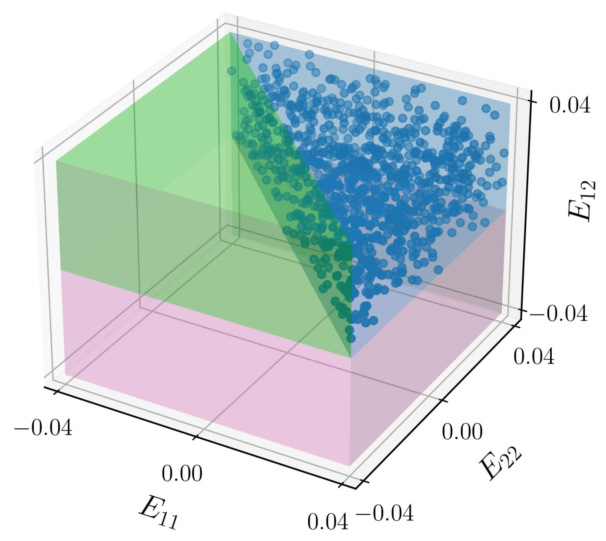We utilized Latin hypercube sampling (LHS) [88] to efficiently sample from the input space. To generate the data, we consider two global symmetries in the input space:

$$\begin{array}{c}\hfill \begin{array}{cc}\hfill T_{12}(E_{11},E_{22},-E_{12})& =-T_{12}(E_{11},E_{22},E_{12}),\hfill \end{array}\end{array}$$

(62)

$$\begin{array}{c}\hfill \begin{array}{cc}\hfill T_{11}(-E_{11},-E_{22},E_{12})& =-T_{11}(E_{11},E_{22},E_{12}),\hfill \\ \hfill T_{22}(-E_{11},-E_{22},E_{12})& =-T_{22}(E_{11},E_{22},E_{12}).\hfill \end{array}\end{array}$$

(63)

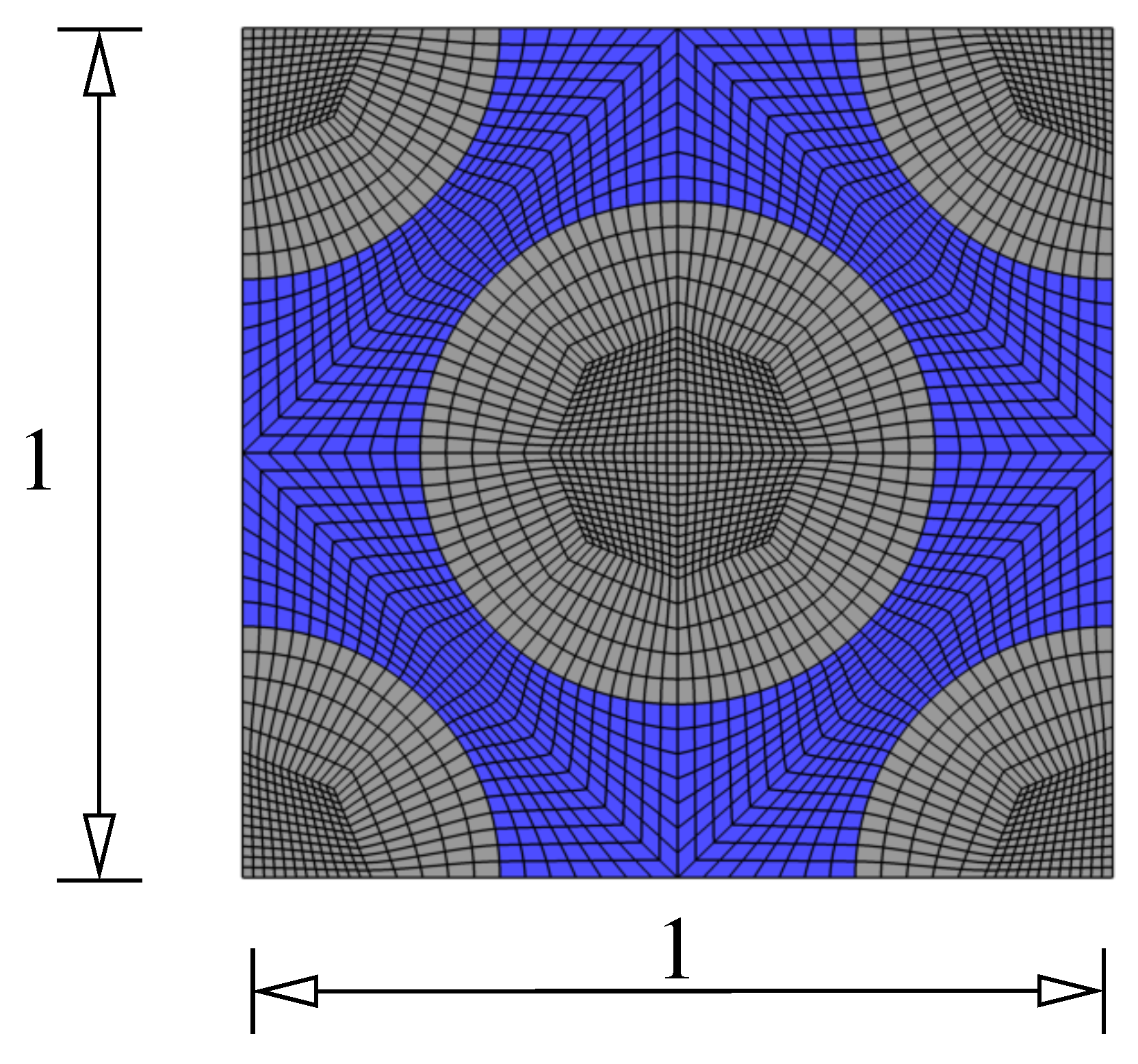
It is important to mention that the assumed symmetries can be employed as long as the materials in the RVE show no tension–compression asymmetry, anisotropy, or rate- or path-dependent behavior, i.e., the reduction in the input space is not applicable for more complex behavior such as plasticity or anisotropic behavior. Thus, the data are generated using the numerical solver for one quarter of the input space according to the region marked by blue in Figure 1.

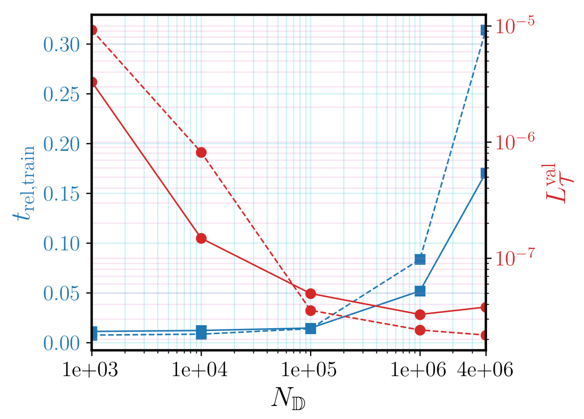
The dataset is augmented by transforming the generated data through the aforementioned global symmetries (62) and (63). This leads to a reduction in the computation time required for the preparation of the training data. After generating the dataset, it is decomposed into 80% for training and 20% for validation. Later on, in Section 4.2, the effect of the size of the training dataset on the accuracy of the final solution obtained from the DNN-based FE${}^2$simulation is investigated. It should be noted that the DNN models are tested by conducting DNN-FE${}^2$simulations and comparing the obtained solutions with those of the reference FE${}^2$ simulations.

3.3. Architecture and Training Process

As it was mentioned in Section 2.2 and Section 3.1, the surrogate model for the local RVE takes $\overline{\mathbf{E}}{\in \mathbb{R}}^3$ as the input and predicts $\overline{\mathbf{T}}{\in \mathbb{R}}^3$ and $\overline{\mathbf{C}}{\in \mathbb{R}}^9$ as the outputs. The obtained stress components and the consistent tangent matrix are assembled at the global finite element level for computation of the next global iteration in the Newton–Raphson method. In this work, two model architectures for our DNN-based surrogate models are considered, both are developed based on MLPs. In the first architecture, two separate neural networks $\mathcal{T}$ and $\mathcal{C}$ are implemented that map $\overline{\mathbf{E}}$ to $\overline{\mathbf{T}}$ and $\overline{\mathbf{C}}$,

$$\overline{\mathbf{T}}=\mathcal{T}(\overline{\mathbf{E}};{\theta }_{\mathcal{T}}),\overline{\mathbf{C}}=\mathcal{C}(\overline{\mathbf{E}};{\mathit{\theta }}_{\mathcal{C}}),$$

(64)

where ${\mathit{\theta }}_{\mathcal{T}}$ and ${\theta }_{\mathcal{C}}$ represent the trainable parameters of deep neural network, $\mathcal{T}$ and $\mathcal{C}$, respectively. The notation in use indicates that the deep neural networks are evaluated for strain inputs $\overline{\mathbf{E}}$ with the given parameters after training the neural network. Throughout the article, this architecture is denoted as NN–2. However, this architecture does not consider that the consistent tangent matrix is the functional matrix of the stress components with respect to the strains,

$$\overline{\mathbf{C}}=\left[C_{ij}\right]\mathrm{with}{C}_{ij}=\frac{\partial T_i}{\partial E_j},i,j=1,2,3,$$

(65)

where $T_i$ and $E_j$ are the corresponding entries in $\overline{\mathbf{T}}$ and $\overline{\mathbf{E}}$, respectively. Thus, this is taken into account in the second architecture by computing $\overline{\mathbf{C}}$ as the output of the Jacobian function ${\mathcal{T}}^{\prime }$ as

$$\overline{\mathbf{T}}=\mathcal{T}(\overline{\mathbf{E}};{\mathit{\theta }}_{\mathcal{T}}),\overline{\mathbf{C}}=\frac{{\displaystyle \partial \mathcal{T}}}{{\displaystyle \partial \overline{\mathbf{E}}}}:={\mathcal{T}}^{\prime }(\overline{\mathbf{E}};{\mathit{\theta }}_{\mathcal{T}}),$$

(66)

where ${\mathcal{T}}^{\prime }$ is obtained by applying reverse mode AD on the deep neural network surrogate $\mathcal{T}$, which is parameterized with trainable parameters ${\mathit{\theta }}_{\mathcal{T}}$. This architecture is denoted as NN–AD. Moreover, this approach is known as the so-called Sobolev training [61] in which both the target and its derivative with respect to the input are considered for supervised learning. Particular explanations regarding the application of Sobolev training in multiscale simulations are provided in [63], while the method is also employed in [60]. By optimizing the parameters of neural networks to approximate not only the function’s outputs but also the function’s derivatives, the model can encode additional information about the target function within its parameters. Therefore, the quality of the predictions, the data efficiency, and generalization capabilities of the learned neural network can be improved.

In the following, we provide a detailed discussion on the data pre-processing, model training, model selection, and hyperparameter tuning.

3.3.1. Data Pre-Processing

We perform a standardization step on both input and outputs of the model to obtain efficient training of the networks using the statistics of the training dataset. A training dataset ${\mathbb{D}}_{\mathrm{train}}={[\overline{\mathbf{E}},\overline{\mathbf{T}},\overline{\mathbf{C}}]}_{\mathrm{train}}$ is considered with its mean and standard deviation over the samples as vectors $\mu$ and $\sigma$, respectively. For training of the NN–2 model, the input and the outputs are standardized independently with their means and standard deviations,

$${\tilde{V}}_i={\displaystyle \frac{V_i-{\mu }_i}{{\sigma }_i}},$$

(67)

where $V_i$ represents the ith component of $\overline{\mathbf{E}}$ or $\overline{\mathbf{T}}$ with the mean and standard deviation ${\mu }_i$ and ${\sigma }_i$, respectively. In contrast, for the NN–AD model, the consistent tangent matrix $\overline{\mathbf{C}}$ should be scaled consistently with the scaling of $\overline{\mathbf{E}}$ and $\overline{\mathbf{T}}$ so that their relationship is preserved. Therefore, scaling (67) is performed for the NN–AD model for the strains and stresses, while the components of $\overline{\mathbf{C}}$ are scaled as

$${\tilde{C}}_{ij}={\displaystyle \frac{\partial {\tilde{T}}_i}{\partial {\tilde{E}}_j}}={\displaystyle \frac{\partial {\tilde{T}}_i}{\partial T_i}}{\displaystyle \frac{\partial T_i}{\partial E_j}}{\displaystyle \frac{\partial E_j}{\partial {\tilde{E}}_j}}={\displaystyle \frac{{\sigma }_j}{{\sigma }_i}}{C}_{ij},i,j=1,2,3.$$

(68)

3.3.2. Training

In the following, a detailed discussion of the training process of all DNNs implemented in this research work is provided. We utilize an extended version of the stochastic gradient descent algorithm, known as Adam [89], for optimizing the parameters of the network during the training process. The weights and biases of the DNN are initialized using the Glorot uniform algorithm [90] and zero initialization, respectively. All the neural networks are trained for 4000 epochs with an exponential decay of learning rate of

$$\eta ={\eta }_{\mathrm{initial}}{\gamma }^{(\mathrm{current}\mathrm{step}/\mathrm{decay}\mathrm{step})},$$

(69)

where $\eta$ represents the learning rate. ${\eta }_{\mathrm{initial}}={10}^{-3}$ is the initial learning rate and $\gamma =0.1$ is the decay rate. Here, a decay step of 1000 is employed. The decay of the learning rate is applied according to Equation (69) every 1000 epochs to obtain a staircase behavior. For different sizes of the training dataset, the batch size is set such that 100 batches are obtained in order to have the same number of training updates for different sizes of the training dataset. The mean squared error (MSE) is utilized as the loss function. For the NN–2 model, the loss for a sample can be obtained as

$$\begin{array}{cc}\hfill L_{\mathcal{T}}(\mathcal{T}(\overline{\mathbf{E}};{\mathit{\theta }}_{\mathcal{T}}),{\overline{\mathbf{T}}}^{\mathrm{ref}})& ={\displaystyle \frac{1}{3}}\sum _{i=1}^3{({\tilde{T}}_i^{\mathrm{ref}}-{\tilde{T}}_i^{\mathrm{pred}}(\overline{\mathbf{E}};{\mathit{\theta }}_{\mathcal{T}}))}^2,\hfill \end{array}$$

(70)

$$\begin{array}{cc}\hfill L_{\mathcal{C}}(\mathcal{C}(\overline{\mathbf{E}};{\mathit{\theta }}_{\mathcal{C}}),{\overline{\mathbf{C}}}^{\mathrm{ref}})& ={\displaystyle \frac{1}{9}}\sum _{i=1}^9{({\tilde{C}}_{ij}^{\mathrm{ref}}-{\tilde{C}}_{ij}^{\mathrm{pred}}(\overline{\mathbf{E}};{\mathit{\theta }}_{\mathcal{C}}))}^2,\hfill \end{array}$$

(71)

where $L_{\mathcal{T}}$ and $L_{\mathcal{C}}$ indicate the loss for the mapping $\mathcal{T}$ and $\mathcal{C}$, respectively. Here, ${\tilde{T}}_i^{\mathrm{ref}}$ denotes the reference stress value and ${\tilde{T}}_i^{\mathrm{pred}}$ is the prediction of the neural network. Accordingly, ${\tilde{C}}_i^{\mathrm{ref}}$ is the reference value in the consistent tangent and ${\tilde{C}}_i^{\mathrm{pred}}$ is the corresponding prediction.

The loss for a data sample for the NN–AD architecture is computed as

$$\begin{array}{cc}\hfill L(\mathcal{T}(\overline{\mathbf{E}};{\mathit{\theta }}_{\mathcal{T}}),{\overline{\mathbf{T}}}^{\mathrm{ref}},{\overline{\mathbf{C}}}^{\mathrm{ref}})& =\alpha L_{\mathcal{T}}(\mathcal{T}(\overline{\mathbf{E}};{\mathit{\theta }}_{\mathcal{T}}),{\overline{\mathbf{T}}}^{\mathrm{ref}})+\beta L_{{\mathcal{T}}^{\prime }}({\mathcal{T}}^{\prime }(\overline{\mathbf{E}};{\mathit{\theta }}_{\mathcal{T}}),{\overline{\mathbf{C}}}^{\mathrm{ref}})\hfill \end{array}$$

(72)

$$\begin{array}{cc}\hfill & =\alpha {\displaystyle \frac{1}{3}}\sum _{i=1}^3{({\tilde{T}}_i^{\mathrm{ref}}-{\tilde{T}}_i^{\mathrm{pred}}(\overline{\mathbf{E}};{\mathit{\theta }}_{\mathcal{T}}))}^2+\beta {\displaystyle \frac{1}{9}}\sum _{i=1}^9{({\tilde{C}}_i^{\mathrm{ref}}-{\tilde{C}}_i^{\mathrm{pred}}(\overline{\mathbf{E}};{\mathit{\theta }}_{\mathcal{T}}))}^2,\hfill \end{array}$$

(73)

where $\alpha$ and $\beta$ are the weighting coefficients for the two components of the loss. In all the cases, the loss for a batch of data is calculated by taking the average of the per-sample losses in the batch.

3.3.3. Model Selection

During the training process of each model, we track the validation loss and save the parameters of the model which lead to the lowest validation loss as the best model parameters. This helps to avoid overfitting of our deep neural networks. As mentioned earlier, the data are decomposed randomly into 80% for training and 20% for validation.

3.3.4. Hyperparameter Tuning

Hyperparameters in machine learning are the parameters that are defined by the user. Their values are set before starting the learning process of the model, such as number of neurons and hidden layers. The values of the hyperparameters remain unchanged during the training process and the following prediction. In machine learning applications, it is important to set the hyperparameters of a model such that the best performance is obtained regarding both prediction and generalization. Here, we perform hyperparameter tuning using a simple grid search algorithm to optimize the model performance on the validation dataset. For this experiment, a dataset with the size of $N_{\mathbb{D}}={10}^5$ is selected. We investigate three hyperparameters, i.e., the number of hidden layers $N_h$, the number of neurons per each hidden layer $N_n$, and the activation function $\phi$, and carry out the hyperparameter tuning for the NN–2 architecture. Further, the same hyperparameters are employed for the NN–AD architecture for the sake of comparability. Moreover, for the NN–AD model, the weighting coefficients of the two components of the loss, $\alpha$ and $\beta$, are studied as well.

Results of the hyperparameter tuning for the number of hidden layers $N_h$, the number of neurons per each hidden layer $N_n$, and the activation function $\phi$ are reported in Appendix A. We observe that a model with eight hidden layers, 128 neurons per each hidden layer, and a swish activation function leads to $L_{\mathcal{T}}^{\mathrm{val}}=3.52\times {10}^{-8}$ and $L_{\mathcal{C}}^{\mathrm{val}}=2.84\times {10}^{-7}$. Moreover, our results show that increasing the model complexity to more than the aforementioned values would not lead to a significant gain in the model accuracy. Thus, we select these model hyperparameters for further analysis.

Other hyperparameters for the NN–AD model are the weighting coefficients $\alpha$ and $\beta$ of the components of the loss, i.e., $L_{\mathcal{T}}$ and $L_{{\mathcal{T}}^{\prime }}$. Here, the effect of the weighting on the obtained validation losses is investigated. The results are reported in

Table 1. Effect of the weighting coefficients $\alpha$ and $\beta$ for the components of the loss (72) on the performance of the NN–AD model.

($\mathit{\alpha }$, $\mathit{\beta }$)	${\mathit{L}}_{\mathcal{T}}^{\mathbf{val}}$	${\mathit{L}}_{{\mathcal{T}}^{\prime }}^{\mathbf{val}}$
(1, 0.01)	$4.84\times {10}^{-8}$	$1.35\times {10}^{-6}$
(1, 1)	$2.20\times {10}^{-8}$	$8.85\times {10}^{-8}$
(1, 100)	$3.55\times {10}^{-8}$	$2.97\times {10}^{-8}$

.

We choose $\alpha =1$ for all the cases and change $\beta$ from $0.01$ to 100. It can be observed that having a small $\beta$ may lead to an imbalanced training where a difference of almost two orders of magnitude between validation losses ${\mathcal{L}}_{\mathcal{T}}$ and ${\mathcal{L}}_{{\mathcal{T}}^{\prime }}$ exists. However, a $\beta$ of one or larger results in a more balanced training leading to validation losses with nearly the same scale. According to the results of this study, we select a model with $\alpha =1$ and $\beta =100$ for further analysis.

4. Numerical Experiments

In this section, the DNN-FE${}^2$approach for the simulation of two canonical test cases in computational solid mechanics is investigated, i.e., an L-profile and Cook’s membrane, and compare the results with those of FE${}^2$reference simulation. The numerical experiments are performed using both architectures, NN-2 as well as NN-AD, to provide a detailed discussion regarding the accuracy and efficiency of the simulations. The results are reported for the accuracy of the simulations, required time for model development (e.g., computational time needed for training), time of numerical simulation, number of load steps, and the total number of global iterations required for reaching the convergence of the FE${}^2$simulation. To this end, the absolute percentage error

$$ϵ={\displaystyle \frac{|V^{\mathrm{ref}}-V^{\mathrm{pred}}|}{\langle \left|V^{\mathrm{ref}}\right|\rangle }}\times 100$$

(74)

is utilized, where V indicates any component of stress or strain tensors $\overline{\mathbf{T}}$ and $\overline{\mathbf{E}}$, respectively. To avoid the division by zero, the absolute mean of the reference solution on the global grid is employed as the denominator, where $\langle ·\rangle$ shows the ensemble average.

All DNN models are trained on an NVIDIA RTX A2000 Laptop GPU with CUDA 12.1. The DNN-FE${}^2$simulations are performed on an 11th Gen Intel(R) Core(TM) i7-11850H @ 2.50GHz CPU with 16 threads. In contrast, the FE${}^2$reference simulations are conducted on a second-Gen Intel(R) Xeon(R) Silver 4216 @ 2.10GHz CPU with 16 processes and one thread per process. The speed-up gain is calculated by dividing the total time of computation required by the FE${}^2$reference simulation by that of the DNN-FE${}^2$ simulation.

4.1. Problem Setup

For the numerical experiments, we restrict ourselves to two-dimensional test cases, where a plane strain case is always assumed. The representative volume element (RVE) under consideration is chosen as a commonly applied geometry in the mechanical analysis of composite materials; see Figure 2.

Here, the fiber volume fraction of the applied RVE is approximately 55%. The fibers are assumed to behave linearly, in an isotropic elastic manner with bulk modulus $K_{\mathrm{f}}$ and shear modulus $G_{\mathrm{f}}$; see

Table 2. Material parameters for elastic fiber and non-linear elastic matrix material in the RVE.

${\mathit{K}}_{\mathbf{f}}$	${\mathit{G}}_{\mathbf{f}}$	${\mathit{K}}_{\mathbf{m}}$	${\mathsf{\alpha }}_1$	${\mathsf{\alpha }}_2$
N mm ${}^{-2}$	N mm ${}^{-2}$	N mm ${}^{-2}$	N mm ${}^{-2}$	-
4.35 × 104	2.99 × 104	4.78 × 103	5.0 × 101	6.0 × 10−2

.

In contrast, the matrix material is modeled with a non-linear elastic material behavior, which is extracted from an originally viscoplastic constitutive model where the shear modulus is deformation-depending; see [91]. The particular stress–strain relation reads

$$\mathbf{T}=K_{\mathrm{m}}\left(\mathrm{tr}\mathbf{E}\right)\mathbf{I}+G_{\mathrm{m}}\left({\mathbf{E}}^{\mathrm{D}}\right){\mathbf{E}}^{\mathrm{D}}\mathrm{with}{G}_{\mathrm{m}}\left({\mathbf{E}}^{\mathrm{D}}\right)=\frac{{\alpha }_1}{{\alpha }_2+\left|\right|{\mathbf{E}}^{\mathrm{D}}{\left|\right|}_2}.$$

(75)

The material parameters for the non-linear elastic material are the bulk modulus $K_{\mathrm{m}}$ and the parameters ${\alpha }_1$ and ${\alpha }_2$; see Table 2. The spatial discretization of the RVE is achieved with ${\check{n}}_{\mathit{e}}^{e\left(j\right)}=3456$ eight-noded quadrilateral elements and ${\check{n}}_{\mathrm{nodes}}^{e\left(j\right)}=10,561$ nodes.

The application of DNN surrogate models in multiscale simulations is studied for two macroscale test cases—L-profile and Cook’s membrane; see Figure 3.

The spatial discretization is achieved with eight-noded quadrilateral elements. As a result, $n_{\mathrm{G}}^e=9$ integration points are present in each macroscale element, which means that $n_{\mathrm{e}}{n}_{\mathrm{G}}^e$ calls of the RVE in Figure 2 are necessary in each global Newton iteration of a FE${}^2$computation. The L-profile is spatially discretized with $n_{\mathrm{e}}=200$ elements and $n_{\mathrm{nodes}}=709$ nodes. For the Cook’s membrane, $n_{\mathrm{e}}=600$ elements and $n_{\mathrm{nodes}}=1901$ nodes are used. The L-profile has a prescribed displacement boundary condition on the top right edge with ${\overline{u}}_2\left(t\right)=-3\mathrm{mm}{\mathrm{s}}^{-1}t$. In contrast, the Cook’s membrane is fixed on the left edge and has an applied displacement boundary condition ${\overline{u}}_2\left(t\right)=2\mathrm{mm}{\mathrm{s}}^{-1}t$ on the right edge.

The initial time-step size of both numerical examples is $\Delta t_0=1\times {10}^{-3}\mathrm{s}$, whereas the simulation is performed for $t\in \left[0,1\right]$. The time discretization is achieved with the Backward–Euler method; see also Remark 1 regarding the time discretization for purely elastic problems. Here, the time-step size $\Delta t$ is not fixed but chosen based on the number of Newton iterations $N_{\mathrm{iter}}$ and the time-step size of the current step $\Delta t_n$,

$$\begin{array}{c}\Delta t_{\mathrm{new}}=\Delta t_n\times \left\{\begin{array}{cc}{f}_{\max }\hfill & \mathrm{if}{N}_{\mathrm{iter}}\le 5,\hfill \\ f_{\min }\hfill & \mathrm{if}{N}_{\mathrm{iter}}>15,\hfill \\ 1\hfill & \mathrm{if}{N}_{\mathrm{iter}}>5\mathrm{and}{N}_{\mathrm{iter}}\le 15.\hfill \end{array}\right.\end{array}$$

(76)

In this work, the quantities $f_{\max }=1.2$ and $f_{\min }=0.3$ are chosen. The termination criteria of the global Newton iteration are applied as

$$\left||\Delta \mathit{u}|\right|\le {\mathrm{tol}}_{\mathit{u}}\mathrm{and}\left|\left|\mathit{G}\left(\mathit{u}\right)\right|\right|\le {\mathrm{tol}}_{\mathit{G}}.$$

(77)

It should be mentioned that the applied tolerance values are rarely reported in current literature to DNN-FE coupling in multiscale applications, which makes it difficult to draw comparisons. In this work, tolerances ${\mathrm{tol}}_{\mathit{u}}=1\times {10}^{-6}$ and ${\mathrm{tol}}_{\mathit{G}}=1\times {10}^{-3}$ are chosen.

4.2. Investigation on the Size of Dataset

Next, the effect of increasing the size of the dataset on the performance of the DNN models as well as the efficiency and accuracy of the DNN-FE${}^2$simulations are assessed. Different sizes of datasets, i.e., $N_{\mathbb{D}}\in \{{10}^3,{10}^4,{10}^5,{10}^6,4\times {10}^6\}$, are considered, while each dataset is generated according to the explanations in Section 3.2. Note that in all the cases, 80% of the samples in the dataset are used for training and 20% for validation. Results are reported for both NN–2 and NN–AD architectures for having a comprehensive comparison. It should also be noted that the efficient size of the dataset depends on the complexity of the model and the mapping that must be learned. Here, results are reported for NN architectures containing eight hidden layers with 128 neurons per each hidden layer and swish as the activation function, which are selected based on the results of hyperparameter tuning; see Section 3.3.4. Figure 4 illustrates the lowest $L_{\mathcal{T}}^{\mathrm{val}}$ obtained during the training of the DNNs using different sizes of the dataset. It can be seen that increasing the size of the dataset from ${10}^3$ to ${10}^5$ leads to a significant reduction in $L_{\mathcal{T}}^{\mathrm{val}}$. However, improvements in the performance of the model are not significant when further increasing $N_{\mathbb{D}}$. We also report the required time of training in Figure 4. The training time $t_{\mathrm{train}}$ is normalized by the computational time $t_{\mathrm{comp},\mathrm{Cook}}^{{\mathrm{FE}}^2}$ needed for FE${}^2$simulation of the Cook’s membrane,

$$t_{\mathrm{rel},\mathrm{train}}={\displaystyle \frac{t_{\mathrm{train}}}{t_{\mathrm{comp},\mathrm{Cook}}^{{\mathrm{FE}}^2}}},$$

(78)

to offer an insight into the cost of developing an NN-based surrogate model for the RVE in comparison with the FE${}^2$reference simulation. As it is expected, increasing $N_{\mathbb{D}}$ results in an increase in the required training time. It can be observed that even for the largest dataset ($N_{\mathbb{D}}=4\times {10}^6$), the training time is much shorter than the computational time of the FE${}^2$simulation. For the dataset with $N_{\mathbb{D}}$ of ${10}^5$, only 1.39% of the computational time of the FE${}^2$simulation is needed for the training of the NN–AD model.

4.3. Numerical Simulations

The numerical results obtained from DNN-FE${}^2$simulations are reported in this section for the L-profile and Cook’s membrane test cases and compared with the FE${}^2$reference simulations regarding accuracy and efficiency. The accuracy of the simulations is estimated by computing the mean and standard deviation of the absolute percentage error, defined in Equation (74), ${ϵ}_{\mathrm{mean}}$ and ${ϵ}_{\mathrm{std}}$, respectively, over all the components of $\overline{\mathbf{E}}$ and $\overline{\mathbf{T}}$ and over all the global grid points. The speed-up gain is computed by dividing the total time of computation for the FE${}^2$reference simulation by that of the DNN-FE${}^2$simulation. Results are reported for different sizes of the dataset $N_{\mathbb{D}}$ and for both architectures NN–2 as well as NN–AD architectures. We refer to the models trained on datasets with different sizes as model–∗ where $\ast \times {10}^3$ shows the size of the dataset.

4.3.1. L-Profile

Results for the simulation of the L-profile test case are summarized in

Table 3. Results of the DNN-FE${}^2$simulation of the L-profile for different sizes of the training/validation dataset.

Model	${\mathit{N}}_{\mathbb{D}}$	${\mathsf{ϵ}}_{\mathbf{mean}}$ (%)	${\mathsf{ϵ}}_{\mathbf{std}}$ (%)	Speed-Up	${\mathit{N}}_{\mathbf{iter}}$	${\mathit{N}}_{\mathit{t}}$
NN–2–1	$1\times {10}^3$	8.79	10.8	232×	104	32
NN–AD–1	$1\times {10}^3$	4.68	8.52	443×	79	30
NN–2–10	$1\times {10}^4$	3.20	4.87	246×	101	32
NN–AD–10	$1\times {10}^4$	0.42	0.69	400×	86	30
NN–2–100	$1\times {10}^5$	2.48	3.68	254×	97	32
NN–AD–100	$1\times {10}^5$	0.21	0.40	462×	73	30
NN–2–1000	$1\times {10}^6$	1.59	2.62	251×	97	31
NN–AD–1000	$1\times {10}^6$	0.20	0.37	452×	76	30
NN–2–4000	$4\times {10}^6$	1.87	2.89	236×	103	32
NN–AD–4000	$4\times {10}^6$	0.15	0.30	462×	73	30

.

It is evident that both DNN surrogate models, NN–2–1 and NN–AD–1, which were trained on a dataset with only 1000 samples, are accurate enough for achieving the convergence of the FE${}^2$simulation. This is also the case for the NN–2–10 model leading to ${ϵ}_{\mathrm{mean}}$ and ${ϵ}_{\mathrm{std}}$ of 3.20% and 4.87%, respectively. Employing the NN–AD–10 model as the DNN surrogate model leads to the convergence of the simulation and provides very accurate results with ${ϵ}_{\mathrm{mean}}$ and ${ϵ}_{\mathrm{std}}$ of 0.42% and 0.69%, respectively. All the DNN-based models trained on larger datasets lead to the convergence of the simulation. Our results show the superior performance of the NN–AD models in comparison with the NN–2 models in all the numerical experiments. For instance, the NN–2–100 model results in ${ϵ}_{\mathrm{mean}}$ and ${ϵ}_{\mathrm{std}}$ of 2.48% and 3.68%, respectively, while the NN–AD–100 model provides more accurate results with ${ϵ}_{\mathrm{mean}}$ and ${ϵ}_{\mathrm{std}}$ of 0.21% and 0.40%, respectively. Moreover, we observe that the NN–AD architecture is more efficient regarding the required size of the dataset where the NN–AD–10 model performs better than the NN–2–4000 model.

Apart from accuracy aspects, the speed-up gain obtained from the DNN-FE${}^2$simulation is of particular interest. In Table 3, it can be observed that a speed-up of 400× can be obtained from the NN–AD–10 model. This huge speed-up gain shows the excellent potential of the DNN-FE${}^2$approach for fast and accurate multiscale simulations of solid materials. Our results show that the NN–AD–4000 model leads to the best performance regarding the accuracy, speed-up, and the required number of iterations. In general, we can observe that the NN–AD architecture is more efficient than the NN–2 architecture regarding the speed-up gain where, for instance, the NN–AD–100 model obtains a speed-up of 462× against 254× of the NN–2–100 model. The models of both architectures require a quite similar number of time-steps $N_t$, which are here load-steps. The lesser number of load-steps for the NN-AD architecture results from the fewer number of Newton iterations, which leads to slightly higher load-step sizes according to Equation (76). Moreover, it is evident that the speed-up of the NN-AD architecture is higher than for the NN-2 architecture. This is caused, on the one hand, by the lesser number of global Newton iterations $N_{\mathrm{iter}}$ because of the higher prediction accuracy of the consistent tangent matrix. On the other hand, in our implementation, the NN-AD model consisting of one feedforward neural network and the backpropagation step for AD is faster to evaluate than the NN-2 model, which comprises two different feedforward neural networks.

Figure 5 and Figure 6 depict the results obtained from the DNN-FE${}^2$simulation using the NN–AD–100 model as the DNN surrogate model in comparison with that of the FE${}^2$reference simulation for all the components of $\overline{\mathbf{E}}$ and $\overline{\mathbf{T}}$, respectively. The reference solution is illustrated on the left panel, the DNN-FE${}^2$solution is in the middle, and the absolute percentage error $ϵ$ is on the right. It can be observed in Figure 5 that for the normal components of the strain tensor, $E_{11}$ and $E_{22}$, a maximum absolute percentage error of 1.03% is achieved which shows excellent performance of our DNN-FE${}^2$approach. For the shear strain $E_{12}$, the error is slightly higher where a maximum absolute percentage error of 4.38% is obtained. The same conclusion can be drawn from Figure 6, where for the normal components of the stress tensor $T_{11}$ and $T_{22}$, the maximum percentage errors are 2.12% and 1.02%, respectively, while for the shear stress, $T_{12}$, the maximum percentage error is slightly higher and is equal to 4.26%.

Moreover, Figure 7 shows the distribution of the absolute percentage error in the solution for the components of $\overline{\mathbf{T}}$ (up) and $\overline{\mathbf{E}}$ (bottom) obtained from the DNN-FE${}^2$simulation using the NN–AD–100 model on all the integration points of the L-profile test case. The green area and the marked percentage indicate the samples with less than 1% of error and their population proportion. We observe that excellent simulation results are obtained where an absolute percentage error of less than 1% is acquired for most of the samples. For instance, it can be observed that 94.06% of the samples have an error of less than 1% in the solution for the shear stress $T_{12}$.

4.3.2. Cook’s Membrane

Furthermore, we apply the DNN-FE${}^2$approach for the simulation of Cook’s membrane test case and compare the obtained solution with that of the reference FE${}^2$.

Table 4. Results of the DNN-FE${}^2$simulation of the Cook’s membrane different for sizes of the training/validation dataset.

Model	${\mathit{N}}_{\mathbb{D}}$	${\mathsf{ϵ}}_{\mathbf{mean}}$ (%)	${\mathsf{ϵ}}_{\mathbf{std}}$ (%)	Speed-Up	${\mathit{N}}_{\mathbf{iter}}$	${\mathit{N}}_{\mathit{t}}$
NN–2–1	$1\times {10}^3$	0.68	0.89	242×	123	32
NN–AD–1	$1\times {10}^3$	0.60	0.71	527×	85	30
NN–2–10	$1\times {10}^4$	0.31	0.44	292×	104	32
NN–AD–10	$1\times {10}^4$	0.09	0.13	542×	84	30
NN–2–100	$1\times {10}^5$	0.19	0.26	287×	104	32
NN–AD–100	$1\times {10}^5$	0.02	0.02	554×	82	30
NN–2–1000	$1\times {10}^6$	0.13	0.16	286×	105	32
NN–AD–1000	$1\times {10}^6$	0.03	0.06	575×	79	30
NN–2–4000	$4\times {10}^6$	0.12	0.17	291×	103	32
NN–AD–4000	$4\times {10}^6$	0.01	0.01	611×	73	30

summarizes the results for models based on the NN–2 and NN–AD architectures trained on datasets with different sizes.

The NN–2–1 and NN–AD–1 models provide a converged solution with less than 1% of error. This is also the case for the NN–2–10 and NN–2–100. Utilizing NN–AD–10 and NN–AD–100 models leads to the convergence of the simulation with excellent accuracy. We obtain ${ϵ}_{\mathrm{mean}}$ and ${ϵ}_{\mathrm{std}}$ of 0.02% using the NN–AD–100 model, which shows the excellent capability of the NN–AD architecture for surrogate modeling of the local macroscale computations. The results show that the NN–AD architecture outperforms the NN–2 architecture in all the tests where, similar to the results obtained for the L-profile, the errors ${ϵ}_{\mathrm{mean}}$ and ${ϵ}_{\mathrm{std}}$ are almost an order of magnitude lower.

The results are also reported regarding the computational efficiency of the proposed framework in Table 4 for the second numerical experiment of Cook’s membrane; see Figure 3B. It can be observed that the NN–AD–10 model obtains a speed-up gain of 542× for this example. The results show that increasing the size of the dataset leads to a more efficient simulation with a lesser number of iterations and lower computational time. The NN–AD–4000 model provides a speed-up of 611× and leads to the convergence of the simulation in 30 time-steps. Compared to the L-profile test case, higher speed-up gain is achieved for the Cook’s membrane. This is due to the fact that the number of elements, which require microscale computations, is three times higher than that of the L-profile. This suggests that utilizing the DNN-FE${}^2$approach for more expensive computations, e.g., three-dimensional problems, could even lead to a higher speed-up gain.

Figure 8 and Figure 9 show the results obtained from the DNN-FE${}^2$simulation employing the NN–AD–100 model as the DNN surrogate model in comparison with that of the FE${}^2$reference simulation for all the components of $\overline{\mathbf{E}}$ and $\overline{\mathbf{T}}$, respectively. It can be observed that for all the components of strain and stress tensors, very accurate results can be obtained. For normal strains $E_{11}$ and $E_{22}$ and the shear strain $E_{12}$, the maximum absolute percentage errors are 0.14%, 0.16%, and 0.18%, respectively. Moreover, for the stress components $T_{11}$, $T_{22}$, and $T_{12}$ the maximum errors are equal to 0.23%, 0.38%, and 0.10%.

We also report the distribution of the absolute percentage errors over all the integration points for Cook’s membrane test case in Figure 10.

For this case, the green area and the marked percentage indicate the samples with less than 0.1% of error and their population proportion. It can be seen that for most of the sample points, an error of less than 0.1% has been obtained. Our results show the excellent capability of the NN–AD models for very accurate and efficient FE${}^2$ simulations.

4.4. Load-Step Size Behavior

Since FE${}^2$computations usually require small initial time-step sizes $\Delta t_0$, the application of certain time-step control schemes is reasonable. In general, the determination of the time-step size $\Delta t_{\mathrm{new}}$ for the following time-step depending on the current time-step size $\Delta t_n$ can be achieved via different methods. In this contribution, we consider the number of (global) Newton iterations $N_{\mathrm{iter}}$ for the load step-size control; see Equation (76).

The step-size behavior, when using a step-size control based on global Newton iterations, is shown for our two numerical experiments in Figure 11.

For the L-profile, the overall step-size behavior is quite similar for both the FE${}^2$reference simulation and with embedding the DNN surrogate model NN–AD–100; see Figure 11A. However, it is evident that the initial time-step size, which is chosen as $\Delta t_0={10}^{-3}\mathrm{s}$, is suitable for the surrogate model, but not for the FE${}^2$reference simulation as the time-step size is rejected multiple times and convergence is initially reached at $\Delta t=9\times {10}^{-5}\mathrm{s}$. The rejections of the initial time-step size, which represents here the initially applied load-step, result from divergence at the global macroscale level.

A similar behavior is observed for the Cook’s membrane and shown in Figure 11B. The first accepted time-step size is $\Delta t=3\times {10}^{-4}\mathrm{s}$, whereas the DNN surrogate already shows convergence at $\Delta t_0={10}^{-3}\mathrm{s}$. In contrast to the L-profile, the step-size behavior shows significant differences. For the reference FE${}^2$simulation of the Cook’s membrane, a certain limit exists, where the step size decreases because of failures in the local-level computations of the MLNA (RVE computations), i.e., the applied load leads to certain limitations in the step-size behavior of the RVEs. However, the DNN-FE${}^2$computation with the embedded DNN surrogate model is successfully converging even for higher step sizes. The different step-size behaviors for L-profile and Cook’s membrane are obtained due to different magnitudes of the strains at each macroscale integration point that result from the loading conditions in Figure 3; see the results in Figure 5 and Figure 8 as well.

As a result, the application of DNN surrogate models is not only possible for load-step size controlled FE${}^2$computations, but it also leads to certain advantages. On the one hand, higher initial load-step sizes are possible and, on the other hand, certain limitations in the load-step size can be overcome and thus larger step sizes can be applied compared to classical FE${}^2$ computations.

5. Speed-Up with JAX and Just-in-Time Compilation

JAX [82] is a Python library developed by Google Research for high-performance numerical computing. It utilizes an updated version of Autograd [92] for automatic differentiation of native Python and NumPy functions. JAX supports reverse-mode differentiation as well as forward-mode differentiation, and the two can be composed arbitrarily to any order. Moreover, JAX uses XLA (accelerated linear algebra) [93] to compile and run NumPy programs on GPUs and TPUs (tensor processing units), which is performed by just-in-time (JIT) compilation and execution of the calls. JAX also allows just-in-time compilation of user-defined Python functions into XLA-optimized kernels using a one-function application programming interface, jit. Compilation and automatic differentiation can be composed arbitrarily, so one can express sophisticated algorithms and obtain maximal performance without leaving Python. These properties allow the implementation of our NN–AD architecture for RVE surrogate modeling efficiently using JAX. In the following, we discuss just-in-time compilation and its application in our DNN-FE${}^2$simulation framework in combination with FORPy [87].

5.1. Just-in-Time Compilation

Just-in-time (JIT) compilation is a technique used in modern programming languages to improve the performance of code execution at runtime. With JIT compilation, the code is compiled from a high-level language into machine code at the moment it is needed, rather than ahead of time. This allows a more efficient use of resources and can lead to significant performance improvements, especially for applications that require repeated execution of the same code. JIT compilers work by analyzing the code being executed and dynamically generating optimized machine code that is tailored to the specific execution context. In particular, when a program is executed, the JIT compiler analyzes the code being executed and identifies hot spots or sections of code that are frequently executed. These sections of code are then compiled into machine code and stored in memory for future use. The next time the same section of code is executed, the JIT compiler can use the pre-compiled machine code instead of interpreting the code again. This leads to significant performance improvements, as the program spends less time interpreting code and more time executing the machine code.

The JIT compiler in JAX is based on XLA, a domain-specific compiler that optimizes numerical computations for modern hardware architectures. With JAX, users can write a Python code that looks like a NumPy code but runs much faster on specialized hardware. This makes JAX an ideal library for scientific computing, machine learning, and other high-performance computing tasks. In addition to JIT compilation, JAX also provides tools for distributed computing and parallelization, making it a versatile library for a wide range of applications.

5.2. Speed-Up with JAX and JIT

JIT compilation is of interest in the DNN-FE${}^2$approach since a repeated execution of the surrogate model in every iteration and for every integration point occurs. Thus, the JIT compilation of the prediction function, which is called from the FORTRAN finite element code through FORPy, allows for more efficient use of resources and can lead to significant performance improvements. To this end, we developed the NN–AD–100 model using JAX and a neural network library and ecosystem for JAX called Flax [94]. Further, the prediction function is compiled using $\mathtt{jax}.\mathtt{jit}$ transformation.

The results are reported in

Table 5. Comparison of JAX and TensorFlow implementations of the surrogate model NN–AD–100 regarding the computational efficiency.

Framework	${\mathit{t}}_{\mathbf{rel},\mathbf{train}}$	Speed-Up for L-Profile	Speed-Up for Cook’s Membrane
TensorFlow	$1.39\times {10}^{-2}$	462×	554×
JAX	$9.49\times {10}^{-3}$	4629×	5853×

, where we compare the computational efficiency of our TensorFlow and JAX implementations. It should be noted that we utilize the same set of hyperparameters and similar training processes for both implementations. It can be seen that the required time of training is shorter for the JAX implementation, and it is equal to $9.49\times {10}^{-3}$ of the computational time required for FE${}^2$simulation of the Cook’s membrane. Moreover, we gain a significant speed-up from the JAX implementation in comparison with the TensorFlow implementation. The speed-up gain for the L-profile and Cook’s membrane test cases are, respectively, equal to 4629× and 5853× for JAX and 462× and 554× for TensorFlow. To the best of the authors’ knowledge, our JAX implementation provides the highest speed-up in the context of DNN-FE${}^2$simulations for non-linear elastic material behavior in the literature.

6. Conclusions

In the present work, a DNN-FE${}^2$approach is explained in detail to significantly accelerate multiscale FE${}^2$simulations. In general, the algorithmic structure of FE${}^2$computations is a Multilevel-Newton algorithm, even for the case of purely elastic material behavior without internal variables. The main source of computational costs are the local macroscale computations, which include the numerous computations of representative volume elements. Thus, in the DNN-FE${}^2$approach, we replace the local macroscale computations by drawing on a deep neural network surrogate model, which is very fast to evaluate after sufficient training. Here, it turns out that using automatic differentiation and Sobolev training to obtain the consistent tangent information is superior to an approach with two deep neural networks for the prediction of stresses and consistent tangent regarding data efficiency and prediction accuracy. Moreover, in step-size-controlled computations, the deep neural network surrogates are able to overcome certain step-size limitations of the FE${}^2$reference computations. For the Cook’s membrane as a particular example in this contribution, we achieve a speed-up factor of more than 5000 compared to a FE${}^2$reference simulation when using just-in-time compilation techniques together with an efficient coupling between different programming codes using the FORPy library. The main advantage of the explained DNN-FE${}^2$approach is that it can be easily implemented to the existing finite element codes since just the evaluation of a surrogate model for each macroscale integration point has to be considered.

References

1. Smit, R.J.; Brekelmans, W.M.; Meijer, H.E. Prediction of the mechanical behavior of nonlinear heterogeneous systems by multi-level finite element modeling. Comput. Methods Appl. Mech. Eng. 1998, 155, 181–192. [Google Scholar] [CrossRef]
2. Feyel, F. Multiscale FE2 elastoviscoplastic analysis of composite structures. Comput. Mater. Sci. 1999, 16, 344–354. [Google Scholar] [CrossRef]
3. Kouznetsova, V.; Brekelmans, W.A.M.; Baajiens, F.P.T. An approach to micro-macro modeling of heterogeneous materials. Comput. Mech. 2001, 27, 37–48. [Google Scholar] [CrossRef]
4. Miehe, C.; Koch, A. Computational micro-to-macro transitions of discretized microstructures undergoing small strains. Arch. Appl. Mech. 2002, 72, 300–317. [Google Scholar] [CrossRef]
5. Miehe, C. Computational micro-to-macro transitions for discretized micro-structures of heterogeneous materials at finite strains based on the minimization of averaged incremental energy. Comput. Methods Appl. Mech. Eng. 2003, 192, 559–591. [Google Scholar] [CrossRef]
6. Kouznetsova, V.; Geers, M.G.D.; Brekelmans, W.A.M. Multi-scale second-order computational homogenization of multi-phase materials: A nested finite element solution strategy. Comput. Methods Appl. Mech. Eng. 2004, 193, 5525–5550. [Google Scholar] [CrossRef]
7. Schröder, J. A numerical two-scale homogenization scheme: The FE2-method. In Plasticity and Beyond: Microstructures, Crystal-Plasticity and Phase Transitions; Schröder, J., Hackl, K., Eds.; Springer: Vienna, Austria, 2014; pp. 1–64. [Google Scholar]
8. Kochmann, J.; Wulfinghoff, S.; Reese, S.; Mianroodi, J.R.; Svendsen, B. Two-scale FE–FFT-and phase-field-based computational modeling of bulk microstructural evolution and macroscopic material behavior. Comput. Methods Appl. Mech. Eng. 2016, 305, 89–110. [Google Scholar] [CrossRef]
9. Düster, A.; Sehlhorst, H.G.; Rank, E. Numerical homogenization of heterogeneous and cellular materials utilizing the finite cell method. Comput. Mech. 2012, 50, 413–431. [Google Scholar] [CrossRef]
10. Bock, F.E.; Aydin, R.C.; Cyron, C.J.; Huber, N.; Kalidindi, S.R.; Klusemann, B. A Review of the Application of Machine Learning and Data Mining Approaches in Continuum Materials Mechanics. Front. Mater. 2019, 6, 110. [Google Scholar] [CrossRef]
11. Brodnik, N.; Muir, C.; Tulshibagwale, N.; Rossin, J.; Echlin, M.; Hamel, C.; Kramer, S.; Pollock, T.; Kiser, J.; Smith, C.; et al. Perspective: Machine learning in experimental solid mechanics. J. Mech. Phys. Solids 2023, 173, 105231. [Google Scholar] [CrossRef]
12. Jin, H.; Zhang, E.; Espinosa, H.D. Recent Advances and Applications of Machine Learning in Experimental Solid Mechanics: A Review. arXiv 2023, arXiv:2303.07647. [Google Scholar] [CrossRef]
13. Johnson, N.; Vulimiri, P.; To, A.; Zhang, X.; Brice, C.; Kappes, B.; Stebner, A. Invited review: Machine learning for materials developments in metals additive manufacturing. Addit. Manuf. 2020, 36, 101641. [Google Scholar] [CrossRef]
14. Kumar, S.; Kochmann, D.M. What Machine Learning Can Do for Computational Solid Mechanics. In Current Trends and Open Problems in Computational Mechanics; Aldakheel, F., Hudobivnik, B., Soleimani, M., Wessels, H., Weißenfels, C., Marino, M., Eds.; Springer International Publishing: Cham, Switzerland, 2022; pp. 275–285. [Google Scholar]
15. Zhang, P.; Yin, Z.Y.; Jin, Y.F. State-of-the-Art Review of Machine Learning Applications in Constitutive Modeling of Soils. Arch. Comput. Methods Eng. 2021, 28, 3661–3686. [Google Scholar] [CrossRef]
16. Kirchdoerfer, T.; Ortiz, M. Data-driven computational mechanics. Comput. Methods Appl. Mech. Eng. 2016, 304, 81–101. [Google Scholar] [CrossRef]
17. Ghaboussi, J.; Garrett, J.H.; Wu, X. Knowledge-Based Modeling of Material Behavior with Neural Networks. J. Eng. Mech. 1991, 117, 132–153. [Google Scholar] [CrossRef]
18. Lefik, M.; Schrefler, B. Artificial neural network as an incremental non-linear constitutive model for a finite element code. Comput. Methods Appl. Mech. Eng. 2003, 192, 3265–3283. [Google Scholar] [CrossRef]
19. Hashash, Y.M.A.; Jung, S.; Ghaboussi, J. Numerical implementation of a neural network based material model in finite element analysis. Int. J. Numer. Methods Eng. 2004, 59, 989–1005. [Google Scholar] [CrossRef]
20. Deshpande, S.; Sosa, R.I.; Bordas, S.P.A.; Lengiewicz, J. Convolution, aggregation and attention based deep neural networks for accelerating simulations in mechanics. Front. Mater. 2023, 10, 1128954. [Google Scholar] [CrossRef]
21. Yao, H.; Gao, Y.; Liu, Y. FEA-Net: A physics-guided data-driven model for efficient mechanical response prediction. Comput. Methods Appl. Mech. Eng. 2020, 363, 112892. [Google Scholar] [CrossRef]
22. Oishi, A.; Yagawa, G. Computational mechanics enhanced by deep learning. Comput. Methods Appl. Mech. Eng. 2017, 327, 327–351. [Google Scholar] [CrossRef]
23. Huang, D.; Fuhg, J.N.; Weißenfels, C.; Wriggers, P. A machine learning based plasticity model using proper orthogonal decomposition. Comput. Methods Appl. Mech. Eng. 2020, 365, 113008. [Google Scholar] [CrossRef]
24. Nguyen, L.T.K.; Keip, M.A. A data-driven approach to nonlinear elasticity. Comput. Struct. 2018, 194, 97–115. [Google Scholar] [CrossRef]
25. Stainier, L.; Leygue, A.; Ortiz, M. Model-free data-driven methods in mechanics: Material data identification and solvers. Comput. Mech. 2019, 64, 381–393. [Google Scholar] [CrossRef]
26. Eggersmann, R.; Kirchdoerfer, T.; Reese, S.; Stainier, L.; Ortiz, M. Model-Free Data-Driven Inelasticity. Comput. Methods Appl. Mech. Eng. 2019, 350, 81–99. [Google Scholar] [CrossRef]
27. González, D.; Chinesta, F.; Cueto, E. Thermodynamically consistent data-driven computational mechanics. Contin. Mech. Thermodyn. 2019, 31, 239–253. [Google Scholar] [CrossRef]
28. Ciftci, K.; Hackl, K. Model-free data-driven simulation of inelastic materials using structured data sets, tangent space information and transition rules. Comput. Mech. 2022, 70, 425–435. [Google Scholar] [CrossRef]
29. Eghbalian, M.; Pouragha, M.; Wan, R. A physics-informed deep neural network for surrogate modeling in classical elasto-plasticity. Comput. Geotech. 2023, 159, 105472. [Google Scholar] [CrossRef]
30. Huber, N.; Tsakmakis, C. Determination of constitutive properties from sperical indentation data using neural networks, Part I: The case of pure kinematic hardening in plasticity laws. J. Mech. Phys. Solids 1999, 47, 1569–1588. [Google Scholar] [CrossRef]
31. Huber, N.; Tsakmakis, C. Determination of constitutive properties from sperical indentation data using neural networks, Part II: Plasticity with nonlinear and kinematic hardening. J. Mech. Phys. Solids 1999, 47, 1589–1607. [Google Scholar] [CrossRef]
32. Villarreal, R.; Vlassis, N.; Phan, N.; Catanach, T.; Jones, R.; Trask, N.; Kramer, S.; Sun, W. Design of experiments for the calibration of history-dependent models via deep reinforcement learning and an enhanced Kalman filter. Comput. Mech. 2023, 72, 95–124. [Google Scholar] [CrossRef]
33. Hamel, C.M.; Long, K.N.; Kramer, S.L.B. Calibrating constitutive models with full-field data via physics informed neural networks. Strain 2022, 59, e12431. [Google Scholar] [CrossRef]
34. Flaschel, M.; Kumar, S.; De Lorenzis, L. Unsupervised discovery of interpretable hyperelastic constitutive laws. Comput. Methods Appl. Mech. Eng. 2021, 381, 113852. [Google Scholar] [CrossRef]
35. Flaschel, M.; Kumar, S.; De Lorenzis, L. Discovering plasticity models without stress data. NPJ Comput. Mater. 2022, 8, 91. [Google Scholar] [CrossRef]
36. Flaschel, M.; Kumar, S.; De Lorenzis, L. Automated discovery of generalized standard material models with EUCLID. Comput. Methods Appl. Mech. Eng. 2023, 405, 115867. [Google Scholar] [CrossRef]
37. Linka, K.; Kuhl, E. A new family of Constitutive Artificial Neural Networks towards automated model discovery. Comput. Methods Appl. Mech. Eng. 2023, 403, 115731. [Google Scholar] [CrossRef]
38. Linka, K.; Hillgärtner, M.; Abdolazizi, K.P.; Aydin, R.C.; Itskov, M.; Cyron, C.J. Constitutive artificial neural networks: A fast and general approach to predictive data-driven constitutive modeling by deep learning. J. Comput. Phys. 2021, 429, 110010. [Google Scholar] [CrossRef]
39. Le, B.A.; Yvonnet, J.; He, Q.C. Computational homogenization of nonlinear elastic materials using neural networks. Int. J. Numer. Methods Eng. 2015, 104, 1061–1084. [Google Scholar] [CrossRef]
40. Liu, Z.; Bessa, M.; Liu, W.K. Self-consistent clustering analysis: An efficient multi-scale scheme for inelastic heterogeneous materials. Comput. Methods Appl. Mech. Eng. 2016, 306, 319–341. [Google Scholar] [CrossRef]
41. Fritzen, F.; Fernández, M.; Larsson, F. On-the-Fly Adaptivity for Nonlinear Twoscale Simulations Using Artificial Neural Networks and Reduced Order Modeling. Front. Mater. 2019, 6, 75. [Google Scholar] [CrossRef]
42. Yang, J.; Xu, R.; Hu, H.; Huang, Q.; Huang, W. Structural-Genome-Driven computing for thin composite structures. Compos. Struct. 2019, 215, 446–453. [Google Scholar] [CrossRef]
43. Mianroodi, J.; Rezaei, S.; Siboni, N.; Xu, B.X.; Raabe, D. Lossless multi-scale constitutive elastic relations with artificial intelligence. NPJ Comput. Mater. 2022, 8, 67. [Google Scholar] [CrossRef]
44. Gupta, A.; Bhaduri, A.; Graham-Brady, L. Accelerated multiscale mechanics modeling in a deep learning framework. Mech. Mater. 2023, 184, 104709. [Google Scholar] [CrossRef]
45. Nguyen-Thanh, V.M.; Trong Khiem Nguyen, L.; Rabczuk, T.; Zhuang, X. A surrogate model for computational homogenization of elastostatics at finite strain using high-dimensional model representation-based neural network. Int. J. Numer. Methods Eng. 2020, 121, 4811–4842. [Google Scholar] [CrossRef]
46. Aldakheel, F.; Elsayed, E.S.; Zohdi, T.I.; Wriggers, P. Efficient multiscale modeling of heterogeneous materials using deep neural networks. Comput. Mech. 2023, 72, 155–171. [Google Scholar] [CrossRef]
47. Kim, S.; Shin, H. Data-driven multiscale finite-element method using deep neural network combined with proper orthogonal decomposition. Eng. Comput. 2023. [Google Scholar] [CrossRef]
48. Eidel, B. Deep CNNs as universal predictors of elasticity tensors in homogenization. Comput. Methods Appl. Mech. Eng. 2023, 403, 115741. [Google Scholar] [CrossRef]
49. Yang, H.; Guo, X.; Tang, S.; Liu, W.K. Derivation of heterogeneous material laws via data-driven principal component expansions. Comput. Mech. 2019, 64, 365–379. [Google Scholar] [CrossRef]
50. Rao, C.; Liu, Y. Three-dimensional convolutional neural network (3D-CNN) for heterogeneous material homogenization. Comput. Mater. Sci. 2020, 184, 109850. [Google Scholar] [CrossRef]
51. Reimann, D.; Nidadavolu, K.; ul Hassan, H.; Vajragupta, N.; Glasmachers, T.; Junker, P.; Hartmaier, A. Modeling Macroscopic Material Behavior With Machine Learning Algorithms Trained by Micromechanical Simulations. Front. Mater. 2019, 6, 181. [Google Scholar] [CrossRef]
52. Göküzüm, F.S.; Nguyen, L.T.K.; Keip, M.A. An Artificial Neural Network Based Solution Scheme for Periodic Computational Homogenization of Electrostatic Problems. Math. Comput. Appl. 2019, 24, 40. [Google Scholar] [CrossRef]
53. Korzeniowski, T.F.; Weinberg, K. Data-driven finite element computation of open-cell foam structures. Comput. Methods Appl. Mech. Eng. 2022, 400, 115487. [Google Scholar] [CrossRef]
54. Xu, R.; Yang, J.; Yan, W.; Huang, Q.; Giunta, G.; Belouettar, S.; Zahrouni, H.; Zineb, T.B.; Hu, H. Data-driven multiscale finite element method: From concurrence to separation. Comput. Methods Appl. Mech. Eng. 2020, 363, 112893. [Google Scholar] [CrossRef]
55. Li, B.; Zhuang, X. Multiscale computation on feedforward neural network and recurrent neural network. Front. Struct. Civ. Eng. 2020, 14, 1285–1298. [Google Scholar] [CrossRef]
56. Fuhg, J.N.; Böhm, C.; Bouklas, N.; Fau, A.; Wriggers, P.; Marino, M. Model-data-driven constitutive responses: Application to a multiscale computational framework. Int. J. Eng. Sci. 2021, 167, 103522. [Google Scholar] [CrossRef]
57. Masi, F.; Stefanou, I. Multiscale modeling of inelastic materials with Thermodynamics-based Artificial Neural Networks (TANN). Comput. Methods Appl. Mech. Eng. 2022, 398, 115190. [Google Scholar] [CrossRef]
58. Masi, F.; Stefanou, I. Evolution TANN and the identification of internal variables and evolution equations in solid mechanics. J. Mech. Phys. Solids 2023, 174, 105245. [Google Scholar] [CrossRef]
59. Kalina, K.A.; Linden, L.; Brummund, J.; Kästner, M. FEANN: An efficient data-driven multiscale approach based on physics-constrained neural networks and automated data mining. Comput. Mech. 2023, 71, 827–851. [Google Scholar] [CrossRef]
60. Feng, N.; Zhang, G.; Khandelwal, K. Finite strain FE2 analysis with data-driven homogenization using deep neural networks. Comput. Struct. 2022, 263, 106742. [Google Scholar] [CrossRef]
61. Czarnecki, W.M.; Osindero, S.; Jaderberg, M.; Swirszcz, G.; Pascanu, R. Sobolev Training for Neural Networks. In Advances in Neural Information Processing Systems; Guyon, I., Luxburg, U.V., Bengio, S., Wallach, H., Fergus, R., Vishwanathan, S., Garnett, R., Eds.; Curran Associates, Inc.: Red Hook, NY, USA, 2017; Volume 30. [Google Scholar]
62. Vlassis, N.N.; Sun, W. Sobolev training of thermodynamic-informed neural networks for interpretable elasto-plasticity models with level set hardening. Comput. Methods Appl. Mech. Eng. 2021, 377, 113695. [Google Scholar] [CrossRef]
63. Vlassis, N.N.; Sun, W. Geometric learning for computational mechanics Part II: Graph embedding for interpretable multiscale plasticity. Comput. Methods Appl. Mech. Eng. 2023, 404, 115768. [Google Scholar] [CrossRef]
64. Ghavamian, F.; Simone, A. Accelerating multiscale finite element simulations of history-dependent materials using a recurrent neural network. Comput. Methods Appl. Mech. Eng. 2019, 357, 112594. [Google Scholar] [CrossRef]
65. Drosopoulos, G.A.; Stavroulakis, G.E. Data-Driven Computational Homogenization Using Neural Networks: FE2-NN Application on Damaged Masonry. J. Comput. Cult. Herit. 2021, 14, 1–19. [Google Scholar] [CrossRef]
66. Yin, M.; Zhang, E.; Yu, Y.; Karniadakis, G.E. Interfacing finite elements with deep neural operators for fast multiscale modeling of mechanics problems. Comput. Methods Appl. Mech. Eng. 2022, 402, 115027. [Google Scholar] [CrossRef] [PubMed]
67. Rocha, I.; Kerfriden, P.; van der Meer, F. Machine learning of evolving physics-based material models for multiscale solid mechanics. Mech. Mater. 2023, 184, 104707. [Google Scholar] [CrossRef]
68. Liu, Z.; Wu, C.; Koishi, M. A deep material network for multiscale topology learning and accelerated nonlinear modeling of heterogeneous materials. Comput. Methods Appl. Mech. Eng. 2019, 345, 1138–1168. [Google Scholar] [CrossRef]
69. Liu, Z.; Wu, C. Exploring the 3D architectures of deep material network in data-driven multiscale mechanics. J. Mech. Phys. Solids 2019, 127, 20–46. [Google Scholar] [CrossRef]
70. Gajek, S.; Schneider, M.; Böhlke, T. An FE–DMN method for the multiscale analysis of short fiber reinforced plastic components. Comput. Methods Appl. Mech. Eng. 2021, 384, 113952. [Google Scholar] [CrossRef]
71. Gajek, S.; Schneider, M.; Böhlke, T. An FE-DMN method for the multiscale analysis of thermomechanical composites. Comput. Mech. 2022, 69, 1–27. [Google Scholar] [CrossRef]
72. Nguyen, V.D.; Noels, L. Micromechanics-based material networks revisited from the interaction viewpoint; robust and efficient implementation for multi-phase composites. Eur. J. Mech. A Solids 2022, 91, 104384. [Google Scholar] [CrossRef]
73. Hughes, T.J.R. The Finite Element Method; Prentice-Hall: Englewood Cliffs, NJ, USA, 1987. [Google Scholar]
74. Hartmann, S.; Quint, K.J.; Hamkar, A.W. Displacement control in time-adaptive non-linear finite-element analysis. ZAMM J. Appl. Math. Mech. 2008, 88, 342–364. [Google Scholar] [CrossRef]
75. Nguyen, V.D.; Béchet, E.; Geuzaine, C.; Noels, L. Imposing periodic boundary condition on arbitrary meshes by polynomial interpolation. Comput. Mater. Sci. 2012, 55, 390–406. [Google Scholar] [CrossRef]
76. Hartmann, S. A remark on the application of the Newton-Raphson method in non-linear finite element analysis. Comput. Mech. 2005, 36, 100–116. [Google Scholar] [CrossRef]
77. Lange, N.; Hütter, G.; Kiefer, B. An efficient monolithic solution scheme for FE2 problems. Comput. Methods Appl. Mech. Eng. 2021, 382, 113886. [Google Scholar] [CrossRef]
78. Rabbat, N.B.G.; Sangiovanni-Vincentelli, A.L.; Hsieh, H.Y. A Multilevel Newton Algorithm with Macromodeling and Latency for the Analysis of Large-Scale Nonlinear Circuits in the Time Domain. IEEE Trans. Circuits Syst. 1979, 26, 733–740. [Google Scholar] [CrossRef]
79. Hoyer, W.; Schmidt, J.W. Newton-Type Decomposition Methods for Equations Arising in Network Analysis. ZAMM Z. Angew. Math. Und Mech. 1984, 64, 397–405. [Google Scholar] [CrossRef]
80. Baydin, A.G.; Pearlmutter, B.A.; Radul, A.A.; Siskind, J.M. Automatic Differentiation in Machine Learning: A Survey. J. Mach. Learn. Res. 2017, 18, 5595–5637. [Google Scholar]
81. Abadi, M.; Barham, P.; Chen, J.; Chen, Z.; Davis, A.; Dean, J.; Devin, M.; Ghemawat, S.; Irving, G.; Isard, M.; et al. Tensorflow: A system for large-scale machine learning. In Proceedings of the 12th USENIX Symposium on Operating Systems Design and Implementation, Savannah, GA, USA, 2–4 November 2016; Volume 16, pp. 265–283. [Google Scholar]
82. Bradbury, J.; Frostig, R.; Hawkins, P.; Johnson, M.J.; Leary, C.; Maclaurin, D.; Necula, G.; Paszke, A.; VanderPlas, J.; Wanderman-Milne, S.; et al. JAX: Composable Transformations of Python+NumPy Programs. 2018. Available online: https://news.ycombinator.com/item?id=22812312 (accessed on 16 July 2023).
83. Müller, J.D.; Cusdin, P. On the performance of discrete adjoint CFD codes using automatic differentiation. Int. J. Numer. Methods Fluids 2005, 47, 939–945. [Google Scholar] [CrossRef]
84. Charpentier, I.; Ghemires, M. Efficient adjoint derivatives: Application to the meteorological model meso-nh. Optim. Methods Softw. 2000, 13, 35–63. [Google Scholar] [CrossRef]
85. Chandrasekhar, A.; Sridhara, S.; Suresh, K. AuTO: A framework for Automatic differentiation in Topology Optimization. Struct. Multidiscip. Optim. 2021, 64, 4355–4365. [Google Scholar] [CrossRef]
86. Rothe, S.; Hartmann, S. Automatic Differentiation for stress and consistent tangent computation. Arch. Appl. Mech. 2015, 85, 1103–1125. [Google Scholar] [CrossRef]
87. Rabel, E.; Rüger, R.; Govoni, M.; Ehlert, S. Forpy: A library for Fortran-Python interoperability. Available online: https://github.com/ylikx/forpy (accessed on 16 July 2023).
88. McKay, M.D.; Beckman, R.J.; Conover, W.J. A Comparison of Three Methods for Selecting Values of Input Variables in the Analysis of Output from a Computer Code. Technometrics 1979, 21, 239–245. [Google Scholar]
89. Kingma, D.P.; Ba, J. Adam: A Method for Stochastic Optimization. arXiv 2017, arXiv:1412.6980. [Google Scholar]
90. Glorot, X.; Bengio, Y. Understanding the difficulty of training deep feedforward neural networks. In Proceedings of the Thirteenth International Conference on Artificial Intelligence and Statistics, Chia Laguna Resort, Sardinia, Italy, 13–15 May 2010; Volume 9, pp. 249–256. [Google Scholar]
91. Hartmann, S. A thermomechanically consistent constitutive model for polyoxymethylene: Experiments, material modeling and computation. Arch. Appl. Mech. 2006, 76, 349–366. [Google Scholar] [CrossRef]
92. Maclaurin, D.; Duvenaud, D.; Adams, R.P. Autograd: Effortless gradients in numpy. In Proceedings of the ICML 2015 AutoML Workshop, Paris, France, 11 July 2015; Volume 238. [Google Scholar]
93. Sabne, A. XLA: Compiling Machine Learning for Peak Performance. 2020. Available online: https://research.google/pubs/pub50530/ (accessed on 16 July 2023).
94. Heek, J.; Levskaya, A.; Oliver, A.; Ritter, M.; Rondepierre, B.; Steiner, A.; van Zee, M. Flax: A Neural Network Library and Ecosystem for JAX. 2023. Available online: https://github.com/google/flax (accessed on 16 July 2023).
Figure 1. Domain of application for the surrogate model. The two global symmetries in the input space, Equations (62) and (63), are marked using pink and green colors, respectively. Blue dots show a subset of the sampled data points using LHS.
Mca 28 00091 g001
Figure 2. Geometry of the RVE (dimensions in mm) used as microstructure in the numerical experiments with fibers (grey) and matrix material (blue).
Mca 28 00091 g002
Figure 3. Spatial discretization and boundary conditions for macroscale test cases. (A) L-profile; (B) Cook’s membrane.
Mca 28 00091 g003
Figure 4. Influence of the size of the dataset N D on training time t rel , train (78) and validation loss L T val (70) (dashed lines corresponds to NN–AD architecture and solid lines to NN–2 architecture).
Mca 28 00091 g004
Figure 5. Reference data (left) and results obtained from DNN-FE 2 simulation (middle) with NN–AD–100 model as well as error measure (74) (right) for the components of strain tensor E ¯ .
Mca 28 00091 g005
Figure 6. Reference data (left) and results obtained from DNN-FE 2 simulation (middle) with NN–AD–100 model as well as error measure (74) (right) for the components of stress tensor T ¯ .
Mca 28 00091 g006
Figure 7. Histograms of the error (74) for the L-profile when applying the NN–AD-100 model. The top and bottom panels illustrate the error for the components of the stress and strain tensors, T ¯ and E ¯ , respectively.
Mca 28 00091 g007
Figure 8. Reference data (left) and results obtained from DNN-FE 2 simulation (middle) with NN–AD–100 model as well as error measure (74) (right) for the components of strain tensor E ¯ .
Mca 28 00091 g008
Figure 9. Reference data (left) and results obtained from DNN-FE 2 simulation (middle) with NN–AD–100 model as well as error measure (74) (right) for the components of stress tensor T ¯ .
Mca 28 00091 g009
Figure 10. Histograms of the error (74) for the Cook’s membrane when applying the NN–AD-100 model. The top and bottom panels illustrate the error for the components of the stress and strain tensors, T ¯ and E ¯ , respectively.
Mca 28 00091 g010
Figure 11. Step-size behavior of DNN-FE 2 simulations (red) with NN–AD–100 model and FE 2 reference simulation (blue), only accepted time-step sizes are shown. (A) L-profile; (B) Cook’s membrane.
Mca 28 00091 g011