Article

Bivariate Generalized Half-Logistic Distribution: Properties and Its Application in Household Financial Affordability in KSA

by
Marwa K. H. Hassan
1 and
Christophe Chesneau
2,*
1
Department of Mathematics, Faculty of Education, Ain Shams University, Cairo 11566, Egypt
2
Department of Mathematics, LMNO, CNRS-Université de Caen, Campus II, Science 3, CEDEX, 14032 Caen, France
*
Author to whom correspondence should be addressed.
Math. Comput. Appl. 2022, 27(4), 72; https://doi.org/10.3390/mca27040072
Submission received: 19 July 2022 / Revised: 16 August 2022 / Accepted: 17 August 2022 / Published: 19 August 2022
(This article belongs to the Special Issue Statistical Inference in Linear Models)

Abstract

:
The generalized half-logistic distribution is ideal to fit the lifetime of some products, such as ball bearings and electrical insulation. In this paper, we aim to extend this scope by creating a motivated bivariate version. We thus introduce the bivariate generalized half-logistic distribution using the Farlie Gumbel Morgenstern (FGM) copula, which is called the FGM bivariate generalized half-logistic distribution (FGMBGHLD for short). In particular, the FGMBGHLD finds application in describing bivariate lifetime datasets that have weak correlations between variables. Some statistical properties and functions of our new distribution, such as the product moments, moment generating function, reliability function, and hazard rate function, are derived. We discuss the maximum likelihood estimation method of the FGMBGHLD parameters. As an application of the FGMBGHLD in reliability, we consider the stress–strength model when the stress and strength random variables are dependent. We also derive the point and interval estimates of the stress–strength coefficient. Finally, we use the data from the household income and expenditure survey of KSA 2018 for Saudi households by administrative region to demonstrate the practicability of the proposed model. A comparison with a modern bivariate Weibull distribution is performed.

1. Introduction

In various fields, such as life testing, reliability, and biological and engineering sciences, there is a need for flexible lifetime distributions with various probability density and hazard rate properties. To this end, Mudholkar et al. (1995) [1] introduced the exponentiated Weibull family of distributions, which includes unimodal distributions with bathtub hazard rates as well as a broader class of monotone hazard rates. Alternative distributions have been examined since, presenting slightly different features. Gupta and Kundu (1999) [2] proposed a generalized exponential distribution. Olopade (2008) [3] considered two distributions, named type-I and type-III generalized half-logistic distributions. Kantam et al. (2014) [4] proposed a type-II generalized half-logistic distribution (GHLD-II for short). For the purpose of this paper, a brief presentation of the GHLD-II is necessary. On the mathematical plan, the probability density function (PDF), cumulative distribution function (CDF), and reliability function of the GHLD-II with scale parameter σ and power parameter μ are given by
f ( x ) = f x ; σ , μ = μ ( 2 e x σ ) μ σ 1 + e x σ μ + 1 , 0 < x < , σ > 0 , μ > 0
F ( x ) = F x ; σ , μ = 1 2 e x σ 1 + e x σ μ
and
R ( x ) = R x ; σ , μ = 2 e x σ 1 + e x σ μ .
Thus, the GHLD-II is developed through the exponentiation of the reliability function of the half-logistic distribution (see Balakrishnan (1985) [5]).
The flexibility of the GHLD-II is mainly in the mode and tail of the distribution, making it an interesting distribution for the modeling of lifetime phenomena. It is proven to define a better model than the exponential, Weibull, and half-logistic models (see Kantam et al. (2014) [4]).
The first objective of this paper is to derive a comprehensive bivariate generalized half-logistic distribution (BGHLD for short) using the copula approach and study its statistical properties, such as PDF, CDF, product moments, moment generating function, and hazard rate function. Many authors discuss the same idea but other distributions; see Almetwally et al. (2020) [6], Almetwally and Muhammed (2020) [7], and Muhammed et al. (2021) [8]. In view of the impact of the GHLD-II in the recent literature, we derive that bivariate versions have a promising future in terms of modeling and data analysis. Now, in order to detail and motivate the construction of our BGHLD, let us present some basics of the notion of the copula. As a first approach, we can say that a copula is a multivariate CDF for which the marginal distribution of each variable is uniform on the interval ( 0 , 1 ) . It describes the dependence between random variables. The definitions below provide more technical details.
Definition 1. 
Let us consider a random vector ( X 1 , , X d ) and the marginal CDFs denoted by F i x = P ( X i < x ) , for i = 1 , , d . Then, using probability integral transform (PIT) for each component, the distribution of the random vector U 1 , , U d = ( F 1 X 1 , , F d ( X d ) ) belongs to the u n i f 0 , 1 d family of distributions, and the copula related to ( X 1 , , X d ) is defined as the joint CDF of ( U 1 , , U d ) , i.e.,
C u 1 , , u d = P ( U 1 u 1 , , U d u d ) ,
with ( u 1 , , u d ) [ 0 , 1 ] d .
Definition 2. 
C : [ 0 , 1 ] d [ 0 , 1 ] is a d-dimensional copula if it is a CDF with
C u 1 , , u i 1 , 0 , u i + 1 , , u d = 0 , C 1 , , u , 1 , , 1 = u ,
with ( u 1 , , u d ) [ 0 , 1 ] d and u [ 0 , 1 ] . In the bivariate case, C : 0 , 1 2 [ 0 , 1 ] is a bivariate copula if C 0 , u = C u , 0 = 0 , C 1 , u = C u , 1 = u and C u 2 , v 2 C u 2 , v 1 C u 1 , v 2 + C ( u 1 , v 1 ) 0 for all 0 u 1 u 2 1 and 0 v 1 v 2 1 .
The Sklar theorem, established by Sklar (1959) [9], is pivotal in copula theory. It states that, for two random variables X 1 and X 2 with marginal CDFs F 1 ( x 1 ) and F 2 ( x 2 ) and marginal PDFS f 1 ( x 1 ) and f 2 ( x 2 ) , respectively, the CDF and PDF of ( X 1 , X 2 ) are given by
F x 1 , x 2 = C ( F 1 x 1 , F 2 ( x 2 ) )
and
f x 1 , x 2 = f ( x 1 ) f ( x 2 ) c ( F 1 x 1 , F 2 ( x 2 ) ) ,
respectively, where c ( u 1 , u 2 ) denotes the copula density related to C ( u 1 , u 2 ) , i.e., c ( u 1 , u 2 ) = 2 C ( u 1 , u 2 ) / ( u 1 u 2 ) .
Gumbel (1960) [10] discussed one of the most popular parametric families of copulas, called the Farlie Gumbel Morgenstern (FGM) copula. The FGM copula and its density are specified by
C u 1 , u 2 = u 1 u 2 ( 1 + θ 1 u 1 1 u 2 ) , 1 θ 1 ,
and
c ( u 1 , u 2 ) = 1 + θ 1 2 u 1 1 2 u 2 ,
respectively. The parameter θ 
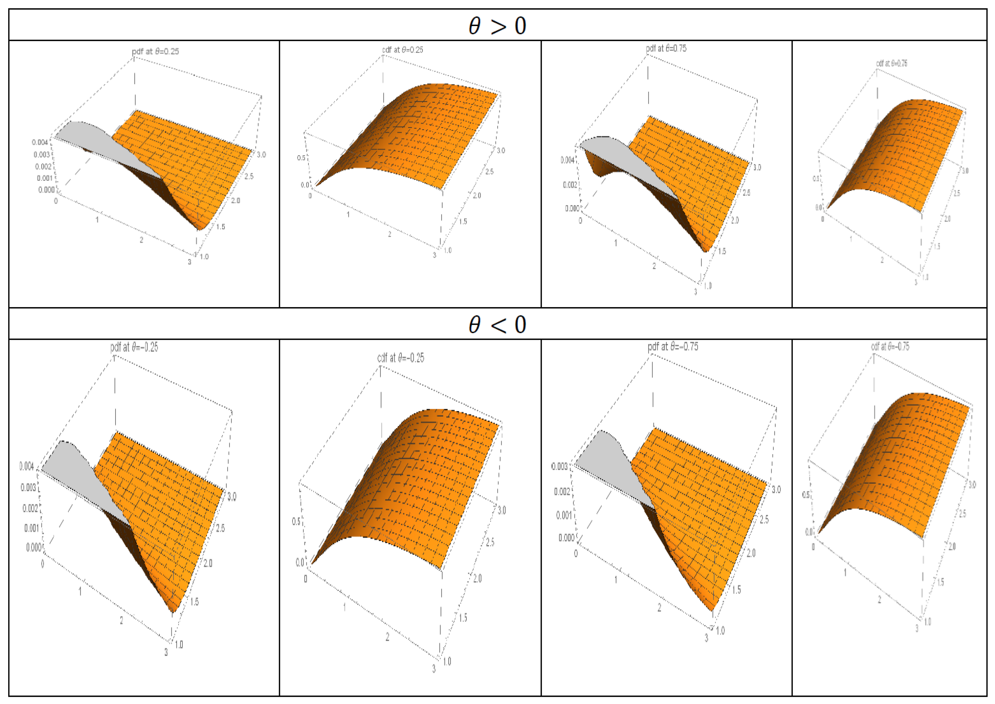
can be thought of as a dependence parameter that is dependent on the underlying random variables, with the independent case being θ = 0 . The FGM copula is thus simple, flexible, and can be adapted when dealing with the construction of bivariate distributions with complicated marginal distributions in terms of functions. It is used in our study to create our BGHLD, which we naturally call the FGMBGHLD.
The second objective is to develop the maximum likelihood (ML) estimation method of the FGMBGHLD parameters. Finally, the third goal is to derive the corresponding stress–strength model, but when and how this makes sense: in the dependent case, which can occur in engineering, operations research, quality control, education, economics, and insurance. Domma and Giordano (2013) [11] provided an example. In this paper, we are interested in economics, where X and Y are household income and consumption, and R = P ( Y < X ) is a measure of household financial affordability.
This paper is organized as follows. In Section 2, the FGMBGHLD is described. In Section 3, we derive some statistical properties of the FGMBGHLD. In Section 4, we exploit the copula approach to take into account the dependence of stress and strength variables in evaluating R. In Section 5, the ML estimation method for the FGMBGHLD parameters is discussed. In Section 6, point and interval estimations for R are elaborated. In Section 7, a Monte Carlo simulation study is performed to study the behavior of different estimates. In Section 8, the estimation of R is applied to KSA data (year 2018) to measure the household financial affordability for Saudi households by administrative region, with comparison to a modern bivariate Weibull distribution. The conclusion of this paper appears in Section 9.

2. FGM Bivariate Generalized Half-Logistic Distribution (FGMBGHLD)

Applying the Sklar theorem as stated in Equations (6) and (7) with Equations (1) and (2), and the FGM copula in Equations (8) and (9), we obtain the CDF and PDF of a random vector ( Y 1 , Y 2 ) following the FGMBGHLD. They are given by
F y 1 , y 2 = 1 2 e y 1 σ 1 1 + e y 1 σ 1 μ 1 1 2 e y 2 σ 2 1 + e y 2 σ 2 μ 2 1 + θ 2 e y 1 σ 1 1 + e y 1 σ 1 μ 1 2 e y 2 σ 2 1 + e y 2 σ 2 μ 2
and
f y 1 , y 2 = μ 1 ( 2 e y 1 σ 1 ) μ 1 σ 1 1 + e y 1 σ 1 μ 1 + 1 μ 2 ( 2 e y 2 σ 2 ) μ 2 σ 2 1 + e y 2 σ 2 μ 2 + 1 1 + θ 2 2 e y 1 σ 1 1 + e y 1 σ 1 μ 1 1 2 2 e y 2 σ 2 1 + e y 2 σ 2 μ 2 1 ,
respectively, with the restrictions of the variables and parameters already mentioned.
In order to illustrate the effect of the dependence parameter θ on the shape of these functions, Figure 1 shows the three-dimensional plots of the PDF and CDF with different values of θ (positive and negative).
From Figure 1, we see that the variable variations of θ play a significant role; the PDF can take different forms in the space, with various skewness and kurtosis.

3. Statistical Properties of the FGMBGHLD

Here, we discuss some statistical properties of the FGMBHLD as defined by Equations (10) and (11). The marginal distributions, product moments, moment generating function, conditional distribution, generating random variables, and reliability function are derived.

3.1. Marginal PDFs

From a random vector ( Y 1 , Y 2 ) following the FGMBHLD, for i = 1 , 2 , the distribution of Y i has the following PDF:
f i y i = 0 f ( y i , y j ) d y j , i j , j = 1 , 2 .
Thus, more concretely, Y 1 has the following PDF:
f 1 y 1 = μ 1 2 e y 1 σ 1 μ 1 σ 1 1 + e y 1 σ 1 μ 1 + 1 , y 1 > 0 , μ 1 , σ 1 > 0
and Y 2 has the following PDF:
f 2 y 2 = μ 2 2 e y 2 σ 2 μ 2 σ 2 1 + e y 2 σ 2 μ 2 + 1 , y 2 > 0 , μ 2 , σ 2 > 0 .
On the other hand, for i j with i , j = 1 , 2 , the general formula for the conditional PDF of Y i given Y j = y j is
f y i y j = f i y i 1 + θ ( 1 2 F i y i ) 1 2 F j y j , 1 θ 1 ,
where F i ( y i ) and F j y j denote the CDFs of Y i and Y j , respectively.
Similarly, the conditional CDF of Y i given Y j = y j is
F y i y j = F i y i 1 + θ 1 F i y i 2 F j y j + 2 F i y i F j y j .
We omit their analytical expressions for the FGMBHLD for the sake of brevity.

3.2. Moment Generating Function

The moment generating function of ( Y 1 , Y 2 ) following the FGMBHLD is obtained as
M Y 1 , Y 2 t 1 , t 2 = E e t 1 Y 1 e t 2 Y 2 = 0 0 e t 1 y 1 e t 2 y 2 f ( y 1 , y 2 ) d y 1 d y 2 = μ 1 μ 2 2 μ 1 + μ 2 ( 1 + t 1 σ 1 ) ( 1 + t 2 σ 2 ) 2 1 + μ 1 θ W 1 2 1 + μ 2 W 2 W 3 W 4 2 1 + μ 2 W 2 1 + θ W 3 ,
where
W 1 = 2 F 1 1 2 μ 1 , 1 t 1 σ 1 ; t 1 σ 1 ; 1 ,
W 2 = 2 F 1 1 2 μ 2 , 1 t 2 σ 2 ; t 2 σ 2 ; 1 ,
W 3 = 2 F 1 1 μ 2 , 1 t 2 σ 2 ; t 2 σ 2 ; 1
and
W 4 = 2 F 1 1 μ 1 , 1 t 1 σ 1 ; t 1 σ 1 ; 1 ,
where 2 F 1 ( a , b ; c ; z ) refers to the (generalized) hypergeometric function.
The parameters t 1 and t 2 must be selected such that the above quantities exist in the mathematical sense, which is the case for t 1 0 and t 2 0 among other more technical cases.

3.3. Product Moments

To obtain the product moments about the origin of ( Y 1 , Y 2 ) following the FGMBHLD, for any positive real numbers r 1 and r 2 , we calculate
μ r 1 r 2 = E Y 1 r 1 Y 2 r 2 = 0 0 y 1 r 1 y 2 r 2 f y 1 , y 2 d y 1 d y 2 ` = μ 1 μ 2 2 μ 1 + μ 2 σ 1 σ 2 A + B + C + D ,
where
A = ( 1 + θ ) s 1 = 0 1 + μ 1 s 1 1 + s 1 σ 1 1 r 1 Γ ( 1 + r 1 ) s 2 = 0 1 + μ 2 s 2 1 + s 2 σ 2 1 r 2 Γ ( 1 + r 2 ) ,
B = θ 2 2 + ( μ 1 + μ 2 ) s 3 = 0 1 + 2 μ 1 s 3 1 + s 3 σ 1 1 r 1 Γ ( 1 + r 1 ) s 4 = 0 1 + 2 μ 2 s 4 1 + s 4 σ 2 1 r 2 Γ ( 1 + r 2 ) ,
C = θ 2 ( μ 1 + 1 ) s 3 = 0 1 + 2 μ 1 s 3 1 + s 3 σ 1 1 r 1 Γ ( 1 + r 1 ) s 2 = 0 1 + μ 2 s 2 1 + s 2 σ 2 1 r 2 Γ ( 1 + r 2 )
and
D = θ 2 ( μ 2 + 1 ) s 1 = 0 1 + μ 1 s 1 1 + s 1 σ 1 1 r 1 Γ ( 1 + r 1 ) s 4 = 0 1 + 2 μ 2 s 4 1 + s 4 σ 2 1 r 2 Γ ( 1 + r 2 ) .
It is understood that Γ ( x ) refers to the standard gamma function, with Γ ( m + 1 ) = m ! for any integer m. From the product moments, various measures of moment skewness and kurtosis can be presented. On this topic, see, for instance, Almetwally et al. (2020) [6], Almetwally and Muhammed (2020) [7], and Muhammed et al. (2021) [8].

3.4. Reliability and Hazard Rate Functions

The reliability function of a bivariate distribution with an associated copula is defined by the copula composed with its marginal reliability functions. See Osmetti and Chiodini (2011) [12]. Hence, based on ( Y 1 , Y 2 ) following the FGMBHLD, it is expressed as
R y 1 , y 2 = C ( R 1 y 1 , R 2 ( y 2 ) ) ,
where R 1 ( y 1 ) and R 2 ( y 2 ) denote the reliability functions of Y 1 and Y 2 , respectively. According to the FGM copula, we obtain
R y 1 , y 2 = R 1 y 1 R 2 y 2 1 + θ 1 R 1 y 1 1 R 2 y 2 , 1 θ 1 .
For the FGMBHLD, the reliability function is
R y 1 , y 2 = 2 e y 1 σ 1 1 + e y 1 σ 1 μ 1 2 e y 2 σ 2 1 + e y 2 σ 2 μ 2 1 + θ 1 2 e y 1 σ 1 1 + e y 1 σ 1 μ 1 1 2 e y 2 σ 2 1 + e y 2 σ 2 μ 2 .
Moreover, Basu (1971) [13] defined the bivariate hazard rate function as
h y 1 , y 2 = f y 1 , y 2 R y 1 , y 2 .
For the FGMBHLD, the hazard rate function is indicated as
h y 1 , y 2 = μ 1 μ 2 σ 1 σ 2 1 + e y 1 σ 1 1 + e y 2 σ 2 1 + θ 2 2 e y 1 σ 1 1 + e y 1 σ 1 μ 1 1 2 2 e y 2 σ 2 1 + e y 2 σ 2 μ 2 1 1 + θ 1 2 e y 1 σ 1 1 + e y 1 σ 1 μ 1 1 2 e y 2 σ 2 1 + e y 2 σ 2 μ 2 .

4. Reliability for Dependence Stress–Strength Model

Domma and Giordano (2013) [11] introduced the concept of dependence via the stress–strength model. They calculated the reliability measure under the hypothesis that the bivariate distribution of the stress and strength variables, modeled by the random variables X and Y, is defined by joining their respective marginal CDFs F ( x ) and G ( y ) for any copula. In this setting, the measure R for dependent X and Y can be defined as
R = P Y < X = 0 0 x c F x , G y f x g y d y d x ,
where f ( x ) and g ( y ) denote the PDFs of X and Y, respectively, and c ( u 1 , u 2 ) the copula density.
Using the FGM copula, we have the following relationship: R = R 1 + θ D , where
R 1 = 0 0 x f x g y d y d x = 0 G x f x d x = E [ G ( X ) ]
and
D = 0 0 x 1 2 F x 1 2 G y d F x d G y = E [ G ( X ) ( 1 G ( X ) ) ( 1 2 F X ) ] .
Now, we calculate R when X and Y have possibly non-identical GHLD with the CDFs F x = 1 2 e x σ 1 + e x σ μ 1 and G y = 1 2 e y σ 1 + e y σ μ 2 , respectively. Hence, σ is common to the two marginal distributions. In this case, after some integral developments, we obtain
R = μ 2 μ 1 + μ 2 + θ μ 1 1 2 μ 1 + μ 2 2 μ 1 + μ 2 + 1 μ 1 + 2 μ 2 .

5. Estimation Method for the Distribution Parameters

In this section, we present the ML method for estimating the FGMBHLD parameters.
Let x 1 , y 1 ( x n , y n ) be a random sample from a random vector ( X , Y ) following the FGMBHLD with the parameters μ 1 , μ 2 , σ 1 , σ 2 , and θ . Hence, in particular, X follows the GBHLD ( μ 1 , σ 1 ) and Y follows the GBHLD ( μ 2 , σ 2 ) . Elaal and Jarwan (2017) [14] introduced the ML estimation method for bivariate distributions based on copula. The basis consists of constructing the log-likelihood function as
L n L = i = 1 n ln f x i g y i c F x i , G y i ,
where F ( x ) and G ( y ) are the CDFs of X and Y, and f ( x ) and g ( y ) are their respective PDFs, and c ( u 1 , u 2 ) refers to the copula density. The ML estimates (MLEs) of the involved parameters are obtained by maximizing this function with respect to these parameters.
Under the setting of the FGMBHLD, we have
L n L = n L n μ 1 + n L n μ 2 + n μ 1 + μ 2 ln 2 μ 1 σ 1 i = 1 n x i μ 2 σ 2 i = 1 n y i n ln σ 1 n ln σ 2 ( μ 1 + 1 ) i = 1 n ln 1 + e x i σ 1 μ 2 + 1 i = 1 n ln 1 + e y i σ 2 + i = 1 n ln ( 1 + θ ϕ x i , μ 1 , σ 1 η y i , μ 2 , σ 2 ) ,
where ϕ x i , μ 1 , σ 1 = 1 2 F ( x i ) and η y i , μ 2 , σ 2 = 1 2 G y i .
The MLEs of the parameters μ 1 , μ 2 , σ 1 , σ 2 and θ , say μ ^ 1 , μ ^ 2 , σ ^ 1 , σ ^ 2 , and θ ^ , are those maximizing this function. They can be obtained by differentiation. To be more precise, by differentiating the log-likelihood with respect to the distribution parameters, we obtain
L n L μ 1 = n μ 1 + n ln 2 1 σ 1 i = 1 n x i i = 1 n ln 1 + e x i σ 1 + i = 1 n θ η y i , μ 2 , σ 2 ϕ μ 1 x i , μ 1 , σ 1 ( 1 + θ ϕ x i , μ 1 , σ 1 η y i , μ 2 , σ 2 ) ,
L n L μ 2 = n μ 2 + n ln 2 1 σ 2 i = 1 n y i i = 1 n ln 1 + e y i σ 2 + i = 1 n θ ϕ x i , μ 1 , σ 1 η μ 2 y i , μ 2 , σ 2 ( 1 + θ ϕ x i , μ 1 , σ 1 η y i , μ 2 , σ 2 ) ,
L n L σ 1 = μ 1 σ 1 2 i = 1 n x i n σ 1 + ( μ 1 + 1 ) σ 1 2 i = 1 n x i e x i σ 1 1 + e x i σ 1 + i = 1 n θ η y i , μ 2 , σ 2 ϕ σ 1 x i , μ 1 , σ 1 1 + θ ϕ x i , μ 1 , σ 1 η y i , μ 2 , σ 2 ,
L n L σ 2 = μ 2 σ 2 2 i = 1 n y i n σ 2 + ( μ 2 + 1 ) σ 2 2 i = 1 n y i e y i σ 2 1 + e y i σ 2 + i = 1 n θ ϕ x i , μ 1 , σ 1 η σ 2 y i , μ 2 , σ 2 ( 1 + θ ϕ x i , μ 1 , σ 1 η y i , μ 2 , σ 2 )
and
L n L θ = i = 1 n ϕ x i , μ 1 , σ 1 η y i , μ 2 , σ 2 1 + θ ϕ x i , μ 1 , σ 1 η y i , μ 2 , σ 2 ,
where
ϕ μ 1 x i , μ 1 , σ 1 = 2 μ 1 + 1 1 1 + e x i σ 1 μ 1 x i σ 1 + ln 2 ln 1 + e x i σ 1 ,
η μ 2 y i , μ 2 , σ 2 = 2 μ 2 + 1 1 1 + e y i σ 2 μ 2 y i σ 2 + ln 2 ln 1 + e y i σ 2 ,
ϕ σ 1 x i , μ 1 , σ 1 = μ 1 x i 2 μ 1 + 1 e x i σ 1 μ 1 1 1 + e x i σ 1 μ 1 σ 1 2 1 + e x i σ 1
and
η σ 2 y i , μ 2 , σ 2 = μ 2 y i 2 μ 2 + 1 e y i σ 2 μ 2 1 1 + e y i σ 2 μ 2 σ 2 2 1 + e y i σ 1 .
By setting the above first partial derivatives of L n L to zero, we obtain μ ^ 1 , μ ^ 2 , σ ^ 1 , σ ^ 2 and θ ^ . Since we cannot obtain a closed form for these estimates, a numerical method must be used.

6. Estimation of the Stress–Strength Distribution Parameter

In this section, we introduce the MLE for R = P ( Y < X ) . Moreover, we derive a motivated asymptotic confidence interval and a bootstrap confidence interval for it.

6.1. Maximum Likelihood Estimate of R

From observed data x 1 , y 1 ( x n , y n ) , which are taken from a random vector ( X , Y ) following the FGMBHLD with the parameters μ 1 , μ 2 , σ 1 , σ 2 , and θ , with σ = σ 1 = σ 2 , we consider the MLEs μ ^ 1 , μ ^ 2 , σ ^ and θ ^ of these parameters, respectively. Then, based on Equation (35) and the invariance property, the MLE of R is obtained by substitution as
R M L E = μ ^ 2 μ ^ 1 + μ ^ 2 + θ ^ μ ^ 1 1 2 μ ^ 1 + μ ^ 2 2 μ ^ 1 + μ ^ 2 + 1 μ ^ 1 + 2 μ ^ 2 .

6.2. Asymptotic Confidence Interval (ACI)

We now aim to compute the ACI for R with a large sample. Let Θ = μ 1 , μ 2 , σ , θ , and Θ i be the i-th component of this vector. First, we construct the Fisher information matrix as follows:
I Θ = I μ 1 , μ 2 , σ , θ = I 11 I 14 I 41 I 44 ,
where I i j = E [ 2 L n L ( X , Y ) Θ i Θ j ] , i , j = 1 , , 4 , Θ i refereing to the ith component of Θ .
Second, we construct the variance–covariance matrix by replacing the distribution parameters by their MLEs, and we obtain
V ^ = V ^ 11 V ^ 14 V ^ 41 V ^ 44 ,
where V ^ i j = 2 L n L Θ i Θ j Θ = Θ ^ , i , j = 1 , , 4 .
To obtain the ACI of R, the following two theorems are useful.
Theorem 1. 
As n , we have
( n μ ^ 1 μ 1 , n μ ^ 2 μ 2 , n σ ^ σ , n θ ^ θ ) N 4 ( 0 , A 1 ) ,
where A = V ^ n .
Proof. 
The theorem can be demonstrated using the asymptotic properties of MLEs of the distribution parameters under regularity conditions and the multivariate central limit theorem. □
Theorem 2. 
As n , we have n R ^ R N ( 0 , B ) , where B = b T A 1 b ,
b = R μ 1 , R μ 2 , R σ , R θ .
Proof. 
The proof is based on Theorem 1 and the application of the delta method. □
According to Xu and Long (2007) [15], a 100 1 α % ACI of R is
R ^ Z α / 2 B ^ n , R ^ + Z α / 2 B ^ n ,
where Z α / 2 denotes the value providing an area of α 2 in the upper tail of the standard normal distribution, and B ^ = b ^ T A 1 b ^ , where b ^ is defined as Equation (51) with substitution of the unknown parameters by the corresponding MLEs.

7. Simulation

In this section, a Monte Carlo simulation study is introduced to describe the point and interval estimation of R .

7.1. Random Variate Generation

Nelsen (2006) [16] discussed the generation of a sample from a specified joint distribution using the conditional distribution method. In the setting of the FGMBHLD, it consists of the following steps:
(i)
Generate u and v independently from a uniform ( 0 , 1 ) distribution.
(ii)
Put y 1 = σ 1 ln ( 1 2 ( 1 u ) μ 1 ) .
(iii)
Put F y 2 y 1 = v to find y 2 using numerical simulation.
(iv)
Repeat (i) to (iii) n-times to obtain ( y 1 j , y 2 j ) , j = 1 , , n .
The obtained n pair of values are thus generated values from ( Y 1 , Y 2 ) following the FGMBHLD.

7.2. Bootstrap Confidence Interval (BCI)

Efron (1982) [17] proposed the bootstrap percentile method (Boot-P) as follows:
(i)
Select the simple random sample x i , y i , i = 1 , , n .
(ii)
Re-sample the simple random sample x i , y i with replacement.
(iii)
Obtain the new simple random sample ( x i * , y i * ) .
(iv)
Compute R * .
(v)
Repeat step (i)–(iv) B-times and compute R 1 * , , R n * .
(vi)
Arrange R 1 * , , R n * , from the smallest to the largest R ( 1 ) * , , R ( n ) * .
(vii)
Construct a 100 1 α % ACI of R as
R α 2 , B * , R 1 α 2 , B * .

7.3. Experiment

1.
Assume some true values of the parameters μ 1 , μ 2 , σ , θ and compute the corresponding true values of R .
Case 1: If μ 1 = 0.5 , μ 2 = 1.5 , σ = 1 , θ = 0.75 , then R = 0.8678 .
Case 2: If μ 1 = 0.5 , μ 2 = 1.5 , σ = 1 , θ = 0.25 , then R = 0.7892 .
Case 3: If μ 1 = 0.5 , μ 2 = 1.5 , σ = 1 , θ = 0.25 , then R = 0.7107 .
Case 4: If μ 1 = 0.5 , μ 2 = 1.5 , σ = 1 , θ = 0.75 , then R = 0.6321 .
2.
Use the algorithm in Section 7.2 to generate different sample sizes with n = 30 , 50 , 70 and 100, with 10,000 replications. All computations are obtained using Mathematica 11.1.
3.
Calculate R M L E according to the methodology in Section 6.1 and the “average R M L E ”, say R M L E * , based on all the samples at a fixed size.
4.
Evaluate the ACI and BCI according to the methodology in Section 6.2 and Section 7.2.
5.
Study the behavior of R M L E by evaluating the bias defined by the “average of R M L E R ” and the mean square error (MSE) indicated as the “average of R M L E R 2 ”.
6.
In the context of interval estimation, we compare the ACI and BCI using the asymptotic confidence length (ACL) and converge probability (CP).
The results of the simulation study are presented in Table 1.
From Table 1, we can conclude that:
1.
At n = 100 , the value of the MSE becomes very small.
2.
In general, the length of the ACI becomes smaller than the length of the BCI.
3.
When the ACL decreases, the CP increases.
4.
The CP in almost all cases of the ACI is more than the CP in the BCI.
Hence, from the above results, the behavior of the MLEs is good for large samples. Moreover, the ACI is more suitable than the BCI for the stress–strength model.

8. Application: Household Financial Affordability in KSA 2018

In this section, we introduce a real application of the stress–strength model in an economic data setting, where X and Y represent household income and consumption, respectively. Here, R = P ( Y < X ) is a household’s financial affordability. We use the data from the household income and expenditure survey of KSA 2018. The survey period was from 28 February 2017 to 31 March 2018 in each month. In this study, we are interested in studying the behavior of R when X represents the average household monthly income by administrative region for Saudi households and Y represents the average household monthly consumption expenditure by administrative region for Saudi households, in order to measure the financial affordability for Saudi households by administrative region in 2018. The data are shown in Table 2. Table 3 presents the descriptive statistics for the data.
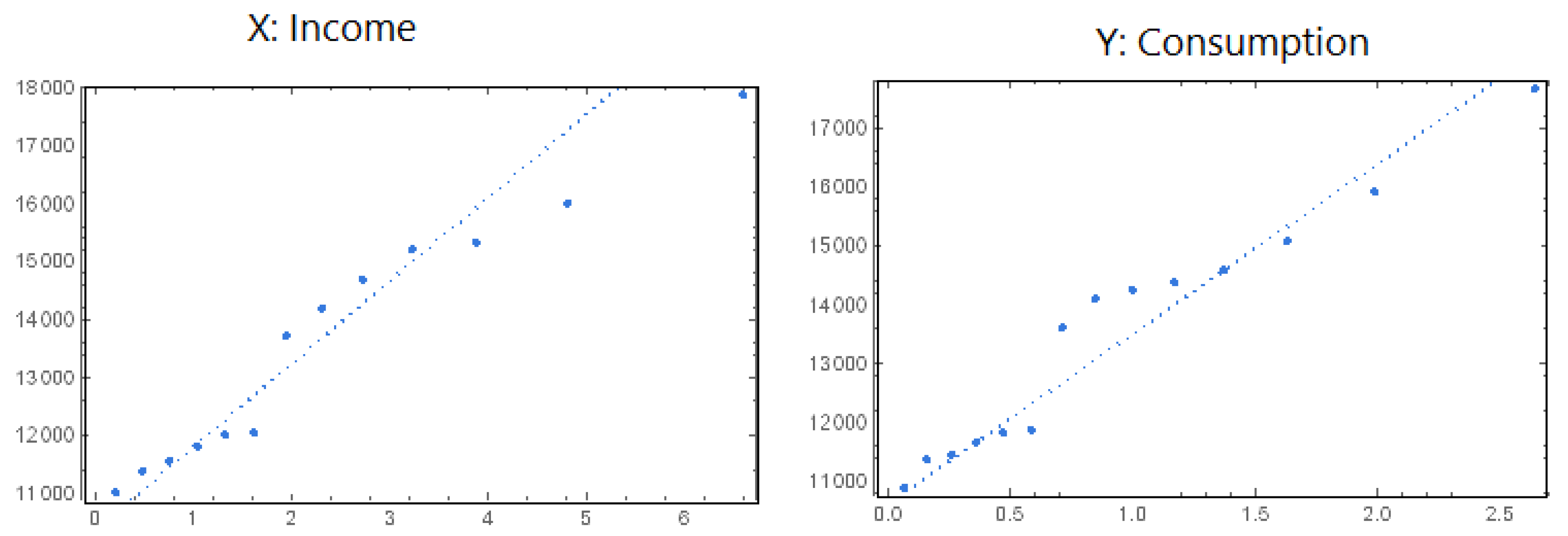
To achieve our aim, we demonstrate the practicability of our proposed model. The Anderson–Darling (AD) goodness of fit statistic value is used to confirm that the GHLD is suitable for the income and consumption data; the corresponding p-values are almost equal to 1. Moreover, the quantile–quantile (Q–Q) plot is used to confirm this statement, as shown in Figure 2.
Now, we evaluate R = P ( Y < X ) in the following two cases:
  • Case 1: If X and Y are independent with X following the GHLD ( μ 1 , σ ) and Y following the GHLD ( μ 2 , σ ) , and the dependent parameter θ is set as 0;
  • Case 2: If X and Y are dependent with ( X , Y ) following the FGMBGHLD.
We calculate, in both cases, the MLEs of the distribution parameters and R, as well as the ACI and ACL. The results are shown in Table 4.
From Table 4, we can conclude that:
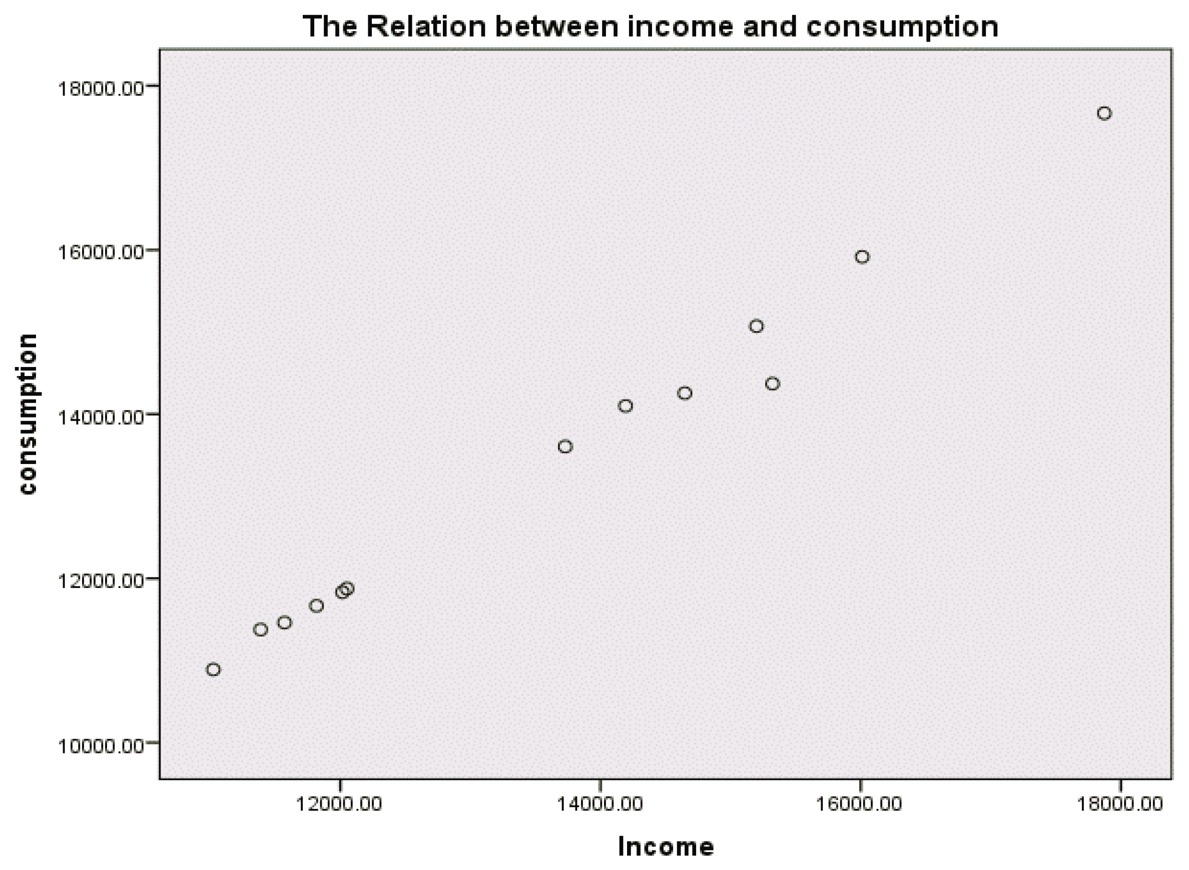
1.
Since θ is estimated as 0.4713 , and is therefore positive, then the relation between X and Y is positive, as we see in
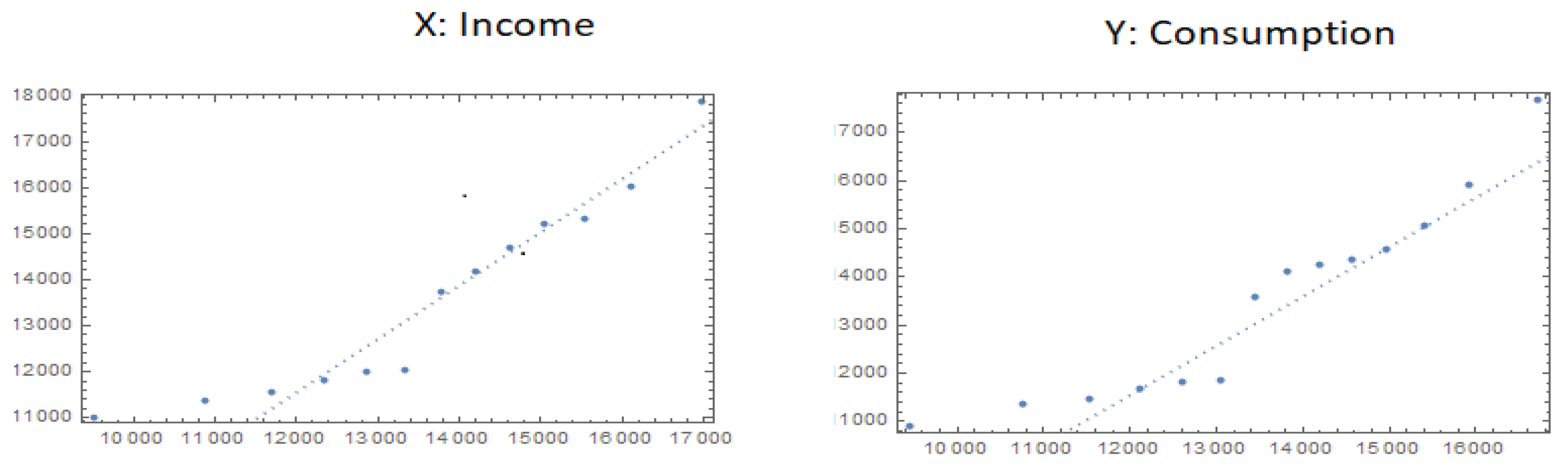
 Figure 3.
2.
The measure of affordability when X and Y are dependent is less than when X and Y are independent, so the case of dependent variables is more realistic.
Figure 3. The scatter plot for the income and consumption of KSA, year 2018.
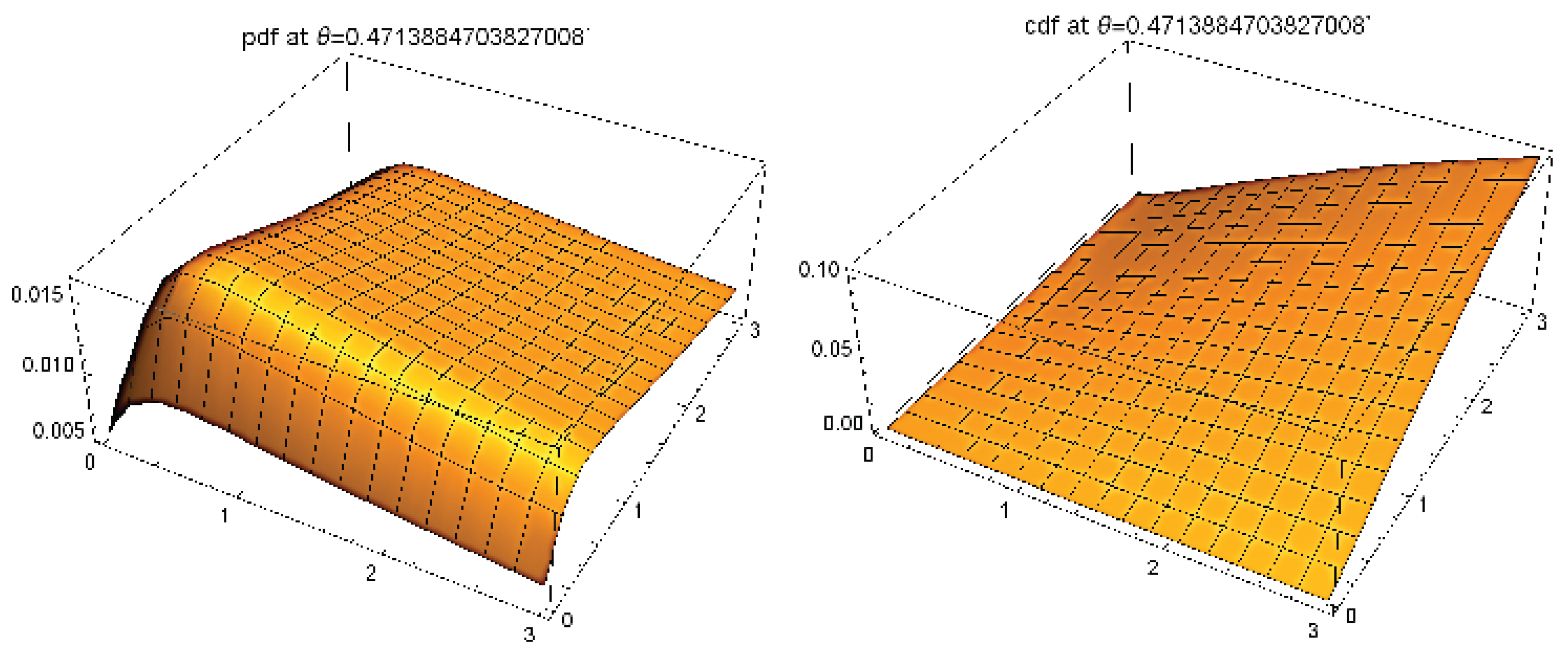
Mca 27 00072 g003
Finally, Figure 4 shows the (estimated) PDF and CDF of the FGMGBHLD with the estimated parameters from the considered data.
It can be noted that the PDF seems unimodal (bump effect) with a long two-dimensional tail. With the FGMBGHLD, the equation behind the calculated PDF and CDF can be employed for further modeling.
To conclude this section, in order to show the performance of our new distribution on KSA data, we compare it with the bivariate Weibull distribution (BWD) as presented in Almetwally et al. (2020) [6]. First, we use the goodness of fit test and Q–Q plot to show that the BWD is a good fit to the KSA data. From the AD goodness of fit test, we find that the p-value equals 0.082 and 0.125 for the two considered data sets, respectively. As a result, the BWD fits the KSA data well. Figure 5 illustrates this conclusion.
Now, we repeat our application but replace our proposed distribution by the BWD. Table 5 shows the result of the MLEs, R, ACIs, and ACLs of the distribution parameters and stress–strength model in the following two cases:
  • Case 1: If X and Y are independent with X following the W e i b u l l ( α 1 , β ) and Y following the W e i b u l l ( α 2 , β ) ;
  • Case 2: If X and Y are dependent with ( X , Y ) following the BWD.
Table 5. The MLEs, ACIs, and ACLs of the BWD parameters for the income and consumption of KSA, year 2018.
CaseMLEMLE for RACIACL
Case 1 α ^ 1 = 6.5
α ^ 2 = 7.5
β ^ = 1.45
0.4642 (0.4631, 0.6461)0.1820
Case 2 α ^ 1 = 6.5
α ^ 2 = 7.5
β ^ = 1.45
θ ^ = 0.1082
0.4275 (0.3456, 0.6058)0.2602
From the ACL viewpoint, we can compare the performance of our distribution and the BWD on the KSA data. Thus, from Table 4 and Table 5, we observe that the ACLs for our proposed distribution are lower than those of the BWD for both cases.
We complete this result by using the AD test for copula-based distributions as described in Genest et al. (2013) [18]. Table 6 shows the p-values of this AD test for our distribution and the BWD (dependent case for both).
The lower p-value is obtained for the FGMBGHLD distribution. Based on the results above, we can confirm that the proposed distribution is more suitable than the BWD for the considered KSA data.

9. Conclusions

In this paper, we introduced the bivariate distribution using the FGM copula approach, abbreviated as FGMBGHLD. We studied some of its statistical properties, such as the PDF, CDF, product moments, moment generating function, reliability function, and hazard rate function. In a multivariate statistical setting (and bivariate in particular), it is well known that the maximum likelihood estimation method gives unique estimates (under some regularity conditions) and guarantees their asymptotic performance from the unbiased and normality viewpoints. For these reasons, we developed it for the FGMBGHLD. We also applied the FGMBGHLD in a real-life data analysis scenario. We investigated the stress–strength model represented by R when the stress and strength variables are dependent and have the FGMBGHLD as a joint distribution. A simulated study was performed to study the behavior of the maximum likelihood estimate of R. Confidence intervals were constructed using two different techniques. Finally, we provided a real application of the considered (dependent) stress–strength model when X and Y measure the household financial affordability in KSA 2018 for Saudi households by administrative region. The obtained results are quite good and competitive with those of a valuable competitor (the bivariate Weibull distribution as introduced by [6]). Research perspectives include the application of the FGMBGHLD to more different bivariate data types, its multivariate version, and the development of regression model types.

Author Contributions

Conceptualization, M.K.H.H. and C.C.; methodology, M.K.H.H. and C.C.; software, M.K.H.H. and C.C.; validation, M.K.H.H. and C.C.; formal analysis, M.K.H.H. and C.C.; investigation, M.K.H.H. and C.C.; resources, M.K.H.H. and C.C.; data curation, M.K.H.H. and C.C.; writing—original draft preparation, M.K.H.H. and C.C.; writing—review and editing, M.K.H.H. and C.C.; visualization, M.K.H.H. and C.C. All authors have read and agreed to the published version of the manuscript.

Funding

This research received no external funding.

Data Availability Statement

Not applicable.

Acknowledgments

Not applicable.

Conflicts of Interest

The authors declare no conflict of interest.

References

  1. Mudholkar, G.S.; Srivastava, D.; Freimer, M. Exponentiated Weibull family: A reanalysis of the bus-motor failure data. Technometrics 1995, 37, 436–445. [Google Scholar] [CrossRef]
  2. Gupta, R.D.; Kundu, D. Generalized exponential distributions. Aust. N. Z. J. Stat. 1999, 41, 173–188. [Google Scholar] [CrossRef]
  3. Olapade, A.K. On Type III Generalized Half Logistic Distribution. arXiv 2008, arXiv:0806.1580v1. [Google Scholar]
  4. Kantam, R.R.L.; Ramakrishna, V.; Ravikumar, M.S. Estimation and Testing in Type-II Generalized Half Logistic Distribution. J. Mod. Appl. Stat. Methods 2014, 13, 267–277. [Google Scholar] [CrossRef]
  5. Balakrishnan, N. Order statistics from the half logistic distribution. J. Stat. Comput. Simul. 1985, 20, 287–309. [Google Scholar] [CrossRef]
  6. Almetwally, E.M.; Muhammed, H.Z.; El-Sherpieny, E.S. Bivariate Weibull Distribution: Properties and Different Methods of Estimation. Ann. Data Sci. 2020, 7, 163–193. [Google Scholar] [CrossRef]
  7. Almetwally, E.M.; Muhammed, H.Z. On a bivariate Fréchet distribution. J. Stat. Appl. Probab. Lett. 2020, 9, 71–91. [Google Scholar]
  8. Muhammed, H.Z.; El-Sherpieny, E.S.; Almetwally, E.M. Dependency Measures For New Bivariate Models Based on Copula Function. Inf. Sci. Lett. 2021, 10, 511–526. [Google Scholar]
  9. Sklar, A. Fonctions de répartition à n dimensions et leurs marges. Publ. Inst. Stat. Univ. Paris 1959, 8, 229–231. [Google Scholar]
  10. Gumbel, E.J. Bivariate exponential distributions. J. Am. Stat. Assoc. 1960, 55, 698–707. [Google Scholar] [CrossRef]
  11. Domma, F.; Giordano, S. A copula-based approach to account for dependence in stress-strength models. Stat. Pap. 2013, 54, 807–826. [Google Scholar] [CrossRef]
  12. Osmetti, S.A.; Chiodini, P.M. A method of moments to estimate bivariate survival functions: The copula approach. Statistica 2011, 71, 469–488. [Google Scholar]
  13. Basu, A.P. Bivariate failure rate. J. Am. Stat. Assoc. 1971, 66, 103–104. [Google Scholar] [CrossRef]
  14. Al Turk, L.I.; Elaal, M.K.A.; Jarwan, R.S. Inference of bivariate generalized exponential distribution based on copula functions. Appl. Math. Sci. 2017, 11, 1155–1186. [Google Scholar] [CrossRef]
  15. Xu, J.; Long, J.S. Using the Delta Method to Construct Confidence Intervals for Predicted Probabilities, Rates, and Discrete Changes. Available online: https://jslsoc.sitehost.iu.edu/stata/ci_computations/spost_deltaci.pdf (accessed on 18 July 2022).
  16. Nelsen, R.B. An Introduction to Copulas; Springer: New York, NY, USA, 2006. [Google Scholar]
  17. Efron, B. The Jackknife, the Bootstrap and Other Re-Sampling Plans. In CBMS-NSF Reginal Conference Series in Applied Mathematics; SIAM: Philadelphia, PA, USA, 1982; Volume 38. [Google Scholar]
  18. Genest, C.; Huang, W.; Dufour, J.M. A regularized goodness-of-fit test for copulas. J. Soc. Fr. Stat. 2013, 154, 64–77. [Google Scholar]
Figure 1. Three-dimensional plots for the PDF and CDF of the FGMBGHLD with different values of θ (for μ 1 = μ 2 = 0.5 , σ 1 = 0.2 and σ 2 = 0.1 ).
Mca 27 00072 g001
Figure 2. Q–Q plot for the income and consumption.
Mca 27 00072 g002
Figure 4. The estimated PDF and CDF of the FGMBGHLD for the income and consumption of KSA, year 2018.
Mca 27 00072 g004
Figure 5. Q–Q plot for the BWD for the income and consumption of KSA, year 2018.
Mca 27 00072 g005
Table 1. Results of the Monte Carlo simulation study.
Sample Size R true R MLE * MLEACIBCI
BiasMSEACLCPACLCP
μ 1 = 0.5 , μ 2 = 1.5 , σ = 1 , θ = 0.75
n = 30 0.86780.3960−0.02280.01570.2050.9350.5980.780
n = 50 0.6463−0.00640.00200.4740.8310.8380.690
n = 70 0.7841−0.00840.00490.3970.8460.8580.684
n = 100 0.3392−0.00370.00140.2230.9800.5030.819
μ 1 = 0.5 , μ 2 = 1.5 , σ = 1 , θ = 0.25
n = 30 0.78920.1027−0.01570.00740.7920.8560.5110.818
n = 50 0.4670−0.00440.00090.4180.8640.4630.842
n = 70 0.1989−0.00110.00010.2510.9260.5240.810
n = 100 0.4110−0.00520.00270.2260.9320.2820.903
μ 1 = 0.5 , μ 2 = 1.5 , σ = 1 , θ = 0.25
n = 30 0.71070.0858−0.02080.01300.1710.9400.7300.731
n = 50 0.3216−0.00770.00300.3670.8610.8060.693
n = 70 0.7090−0.00010.00010.5370.9800.0950.970
n = 100 0.6757−0.00030.00010.0990.9670.1260.960
μ 1 = 0.5 , μ 2 = 1.5 , σ = 1 , θ = 0.75
n = 30 0.63210.66300.00100.00000.2720.9120.1890.941
n = 50 0.5554−0.00150.00010.3080.8940.1940.922
n = 70 0.2641−0.00520.00190.2910.8870.1360.946
n = 100 0.67750.00040.00000.1080.9650.09310.970
Table 2. Average household monthly income (X) and consumption expenditure (Y) by administrative region for Saudi households in 2018.
Administrative RegionIncomeConsumption
Riyadh16,01115,917
Makkah14,64814,256
Madinah12,016118,322
Al-Qassim15,32214,371
Eastern Region17,87217,665
Asir11,81711,666
Tabuk11,02410,890
Hail11,57111,461
North Board12,05111,876
Jazan15,19915,071
Najran11,38811,376
Al-Baha13,72813,605
Aljouf14,19314,101
Total14,82314,584
Table 3. Descriptive statistics for the income and consumption.
MeasureIncomeConsumption
Min11,02410,890
Max17,87217,665
Median13,72813,605
SE592.605574.401
Skewness0.5290.637
Kurtosis−0.686−0.378
Mean13,603.07613,391.307
Table 4. The MLEs, ACIs, and ACLs of the distribution parameters for the income and consumption.
CaseMLEMLE for RACIACL
Case 1 μ ^ 1 = 0.0143
μ ^ 2 = 0.0270
σ ^ = 0.3529
0.3462 (0.2979, 0.3945)0.0965
Case 2 μ ^ 1 = 0.0135
μ ^ 2 = 0.0201
σ ^ = 0.1403
θ ^ = 0.4713
0.2149 (0.1248, 0.3050)0.1802
Table 6. AD test for the proposed distribution and the BWD.
Distributionp-Value
FGMBGHLD0.4999
BWD0.2067
Publisher’s Note: MDPI stays neutral with regard to jurisdictional claims in published maps and institutional affiliations.

