
Modeling the Spread of COVID-19 in Enclosed Spaces


Abstract
:1. Introduction
2. Materials and Methods
2.1. Gammaitoni and Nucci Model
Wells–Riley Equation
2.2. G–N Extension
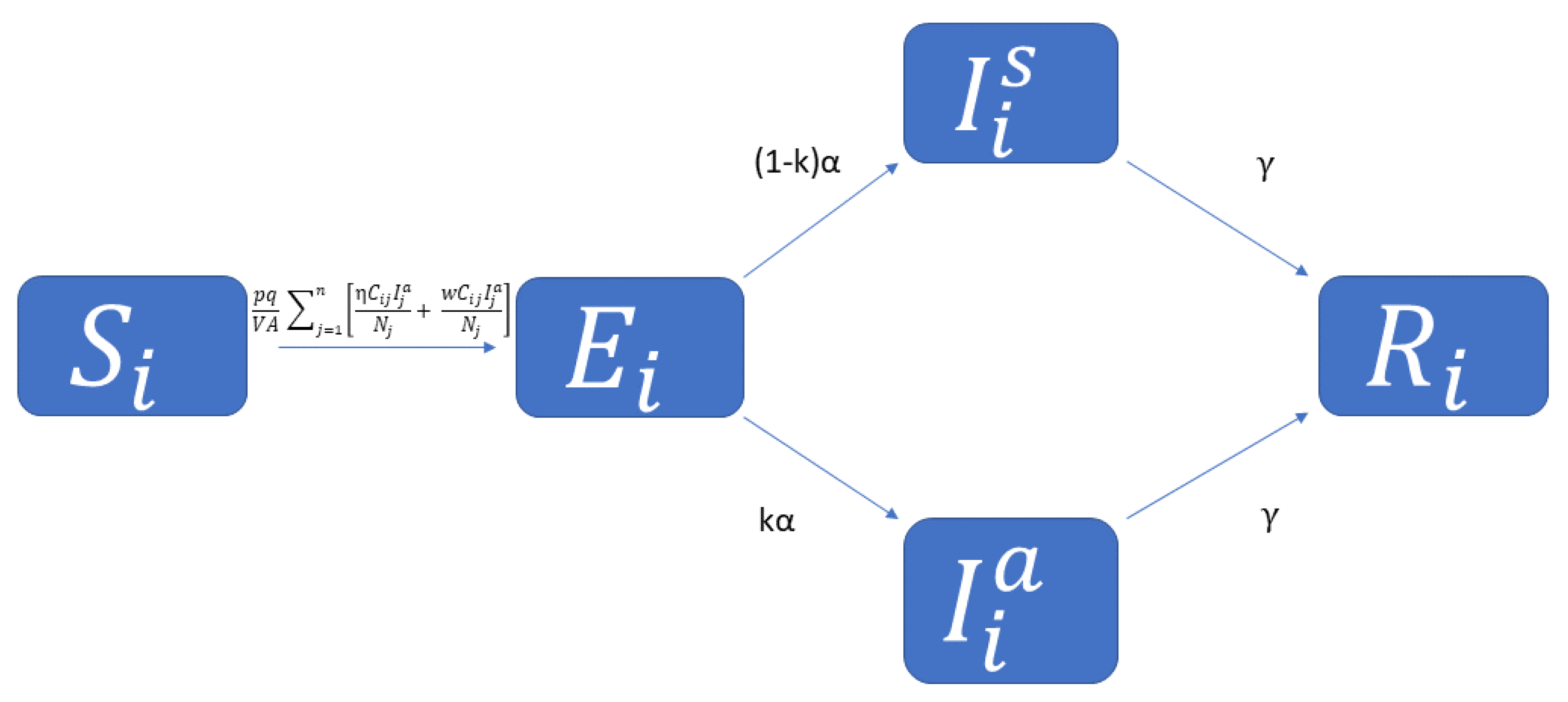
2.3. SEIR Model
2.4. Incubation Period
2.5. Combining Gammaitoni–Nucci and SEIR
2.6. Multi-Age SIR Model
2.7. General Contact Matrix
2.8. Combining G–N and Age-Structured SEIR
2.9. Next Generation Matrix
2.10. Transmission and Transition Matrices
3. Results
3.1. Creating for Proposed Model
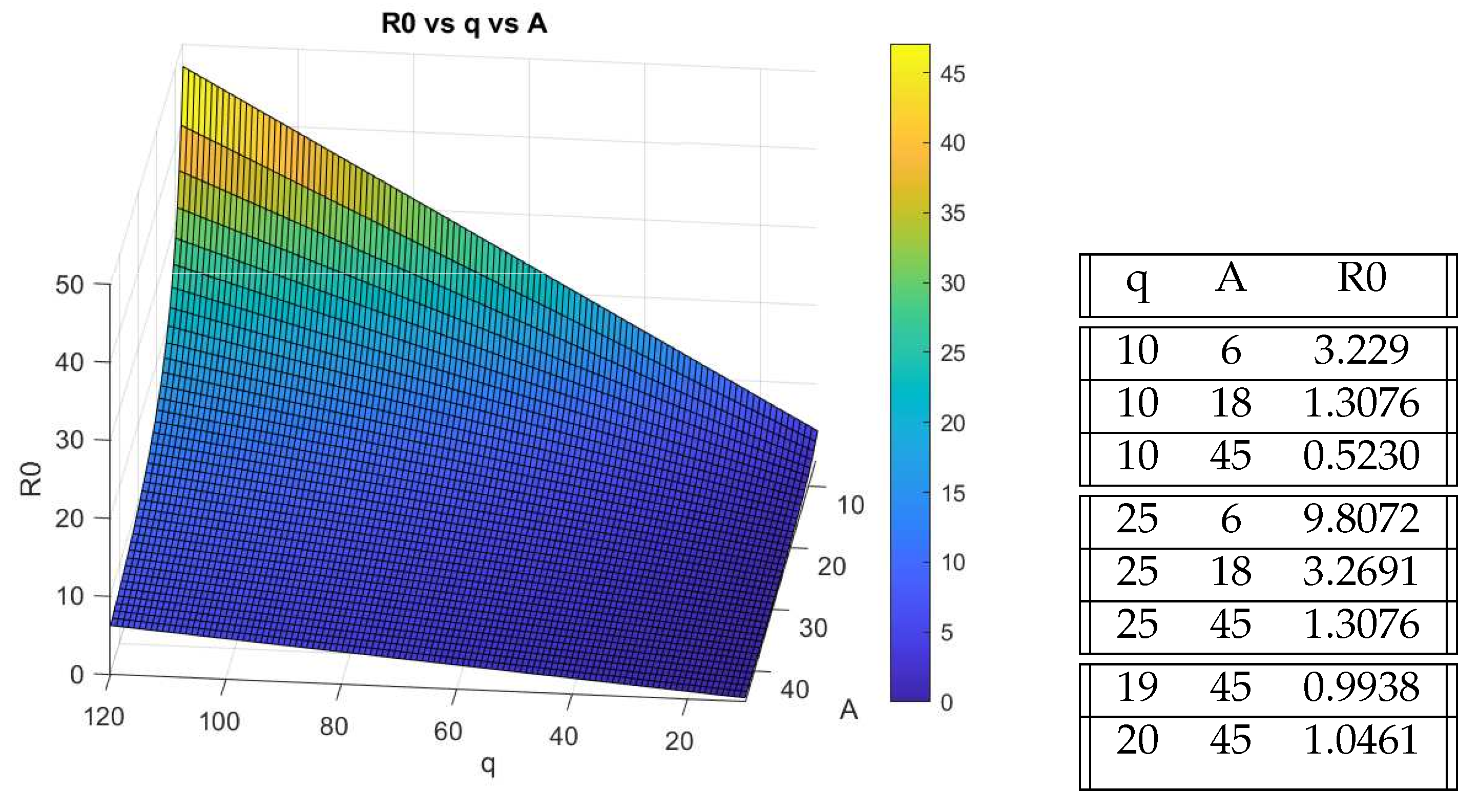
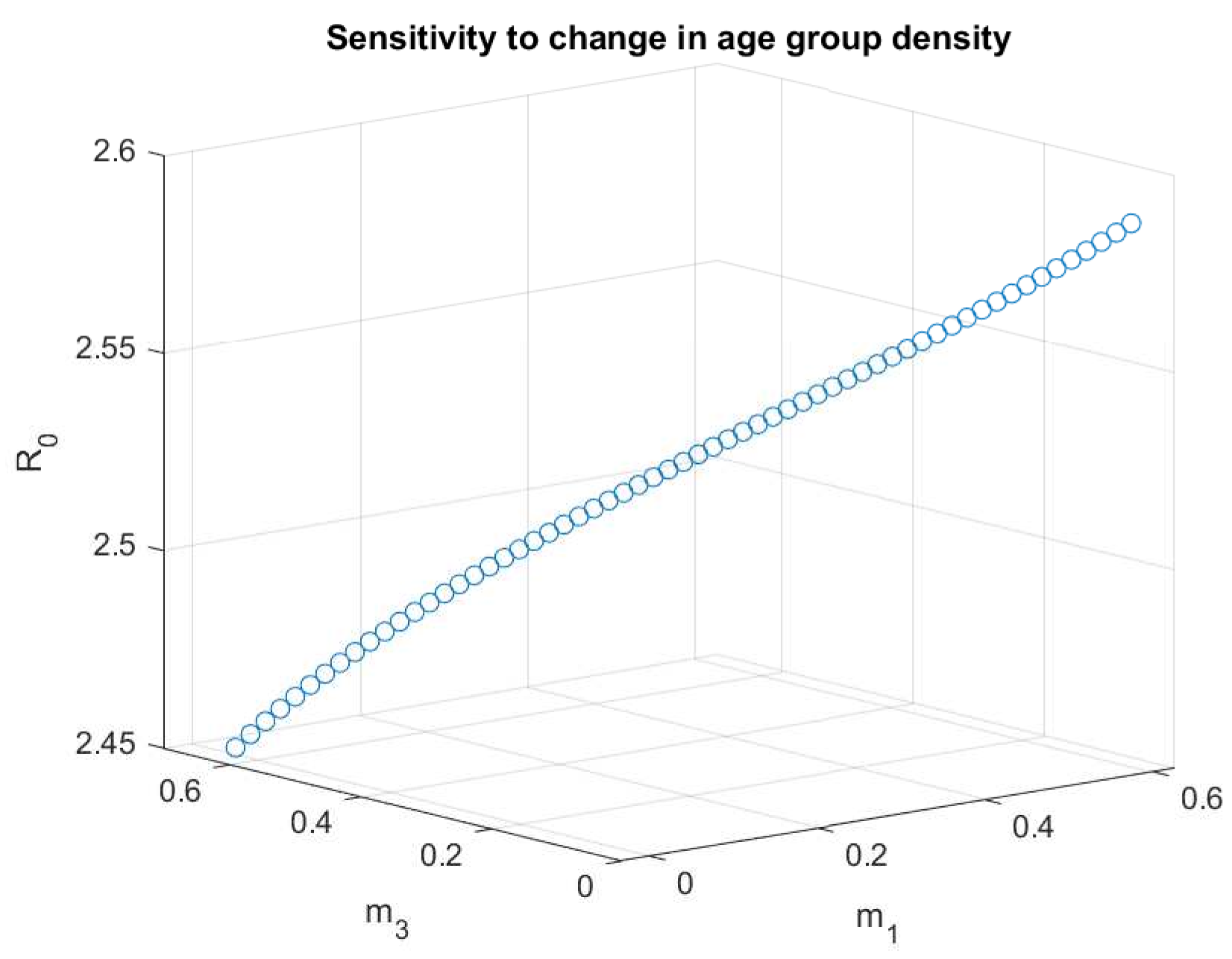
3.2. Parameter Sensitivity Analysis
3.3. Stability Analysis
Elderly Care Facility
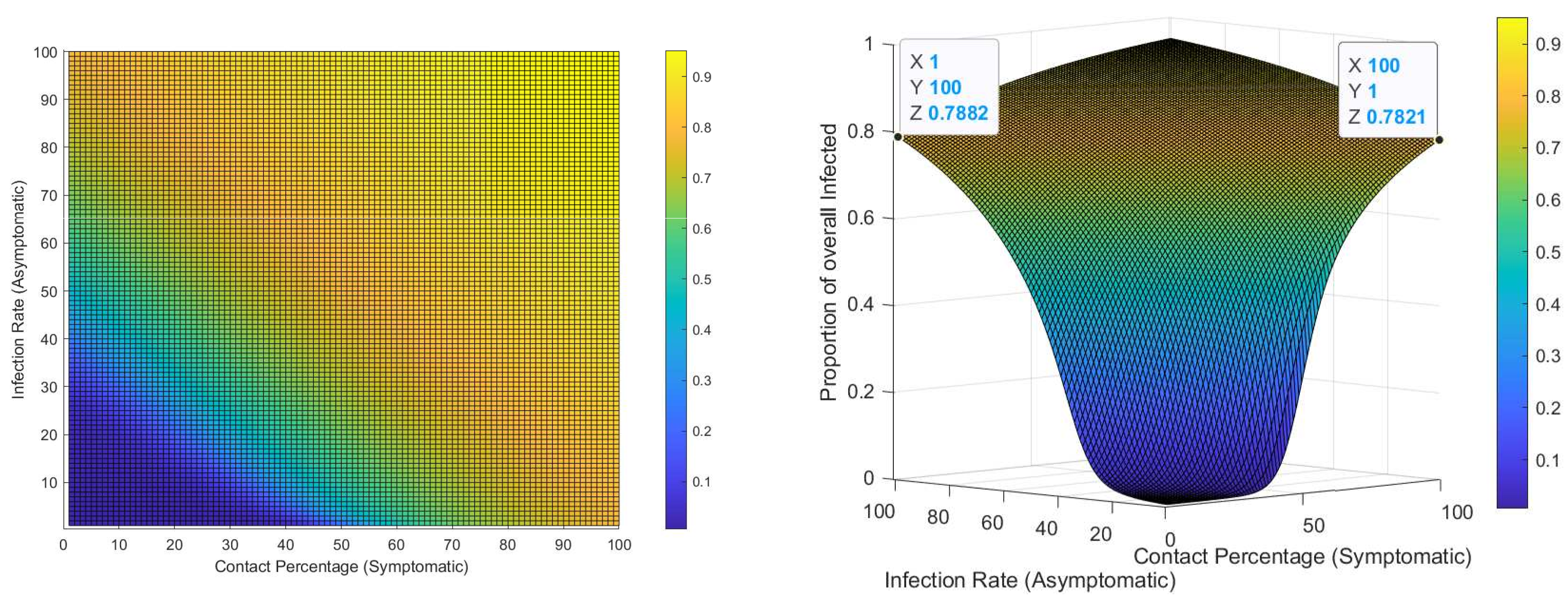
3.4. Initial Infector and Contact Rate
4. Conclusions
Further Research
Author Contributions
Funding
Data Availability Statement
Conflicts of Interest
Abbreviations
| COVID-19 | Coronavirus disease of 2019 |
| G–N Model | Gammaitoni–Nucci Model |
| ACH | Air changes per hour |
| SIR | Susceptible-Infected-Removed |
| SEIR | Susceptible-Exposed-Infected-Removed model |
| NGM | Next Generation Matrix |
Appendix A. Mossong Data Tables

| All Reported Contacts (Physical and Non-Physical Contacts) | |||||||||||||||
|---|---|---|---|---|---|---|---|---|---|---|---|---|---|---|---|
| Age Group of Participant | |||||||||||||||
| Age of Contact | 00-04 | 05–09 | 10–14 | 15–19 | 20–24 | 25–29 | 30–34 | 35–39 | 40–44 | 45–49 | 50–54 | 55–59 | 60–64 | 65–69 | 70+ |
| 00–04 | 2.375 | 0.89875 | 0.27 | 0.18125 | 0.27 | 0.50375 | 0.82375 | 0.65625 | 0.68375 | 0.3225 | 0.2425 | 0.2775 | 0.32875 | 0.1875 | 0.15875 |
| 05–09 | 1.1975 | 6.65625 | 1.1275 | 0.365 | 0.21875 | 0.45375 | 0.92625 | 0.97125 | 0.7 | 0.34625 | 0.46875 | 0.3525 | 0.25875 | 0.315 | 0.2175 |
| 10–14 | 0.44875 | 1.31625 | 9.3 | 1.3725 | 0.2875 | 0.2675 | 0.66 | 0.75125 | 0.91125 | 0.55625 | 0.64125 | 0.37125 | 0.31 | 0.22125 | 0.4 |
| 15–19 | 0.26375 | 0.33 | 1.62 | 9.05875 | 1.56625 | 0.62375 | 0.53875 | 0.53 | 0.99 | 1.225 | 0.77125 | 0.49875 | 0.31125 | 0.20625 | 0.42375 |
| 20–24 | 0.38125 | 0.27125 | 0.4 | 1.45625 | 3.71375 | 1.68875 | 0.79625 | 0.7075 | 1.0225 | 0.89625 | 1.01 | 0.65125 | 0.4475 | 0.305 | 0.2475 |
| 25–29 | 0.7725 | 0.6525 | 0.3875 | 0.67 | 1.89875 | 2.47625 | 1.59125 | 1.16625 | 1.00375 | 1.03875 | 1.29125 | 0.91875 | 0.7125 | 0.5825 | 0.40375 |
| 30–34 | 1.15375 | 0.96625 | 0.58625 | 0.52 | 1.31875 | 1.65875 | 2.36625 | 1.54875 | 1.37375 | 1.18 | 1.06 | 1.075 | 1.0075 | 0.6875 | 0.4325 |
| 35–39 | 1.03 | 1.19875 | 0.9925 | 0.8025 | 0.945 | 1.2 | 2.03875 | 2.4175 | 1.5475 | 1.33875 | 1.06875 | 0.93125 | 0.97375 | 0.86375 | 0.5025 |
| 40–44 | 0.6375 | 1.1225 | 1.31125 | 0.995 | 0.855 | 0.995 | 1.4875 | 2.0125 | 2.13125 | 1.5275 | 1.215 | 1.12 | 0.9275 | 0.86 | 0.67625 |
| 45–49 | 0.40625 | 0.5175 | 0.84875 | 1.2 | 1.0675 | 0.925 | 1.00625 | 1.25625 | 1.545 | 1.86375 | 1.34125 | 1.00125 | 0.73375 | 0.5625 | 0.7 |
| 50–54 | 0.43 | 0.40625 | 0.46875 | 0.6175 | 0.87125 | 1.01875 | 0.87375 | 0.98625 | 1.1425 | 1.31 | 1.46125 | 1.23 | 0.76125 | 0.59375 | 0.5325 |
| 55–59 | 0.39625 | 0.3175 | 0.26875 | 0.335 | 0.4725 | 0.66625 | 0.6325 | 0.56 | 0.4525 | 0.6975 | 1.0775 | 1.55125 | 1.06875 | 0.65375 | 0.4675 |
| 60–64 | 0.3325 | 0.29875 | 0.18 | 0.1575 | 0.2225 | 0.37875 | 0.4875 | 0.57125 | 0.425 | 0.41 | 0.57875 | 0.825 | 1.12125 | 0.83375 | 0.59375 |
| 65–69 | 0.2425 | 0.21375 | 0.17625 | 0.1275 | 0.13 | 0.18875 | 0.25875 | 0.4125 | 0.30125 | 0.21375 | 0.24125 | 0.47375 | 0.695 | 0.90125 | 0.66125 |
| 70+ | 0.31625 | 0.35875 | 0.3625 | 0.25 | 0.315 | 0.35875 | 0.37625 | 0.4375 | 0.56125 | 0.685 | 0.70875 | 0.72375 | 0.89 | 1.05 | 1.45 |
| 4 Categories | 0–19 | 20–39 | 40–59 | 60+ |
|---|---|---|---|---|
| 0–19 | 36.78125 | 10.04875 | 9.35875 | 3.33875 |
| 20–39 | 12.24125 | 27.5325 | 17.4075 | 7.16625 |
| 40–59 | 10.27875 | 15.68625 | 20.6675 | 8.5375 |
| 60+ | 3.01625 | 4.1375 | 6.1475 | 8.19625 |
Appendix B. NGM Submatrices
Appendix C. COVID-19 Statistics


References
- Rosenwald, M.S. History’s Deadliest Pandemics, from Ancient Rome to Modern America. Available online: https://www.spokesman.com/stories/2020/apr/15/historys-deadliest-pandemics-from-ancient-rome-to-/ (accessed on 9 November 2021).
- Davidson, H. First COVID-19 Case Happened in November, China Government Records Show—Report. 2020. Available online: https://www.theguardian.com/world/2020/mar/13/first-COVID-19-case-happened-in-november-china-government-records-show-report (accessed on 9 November 2021).
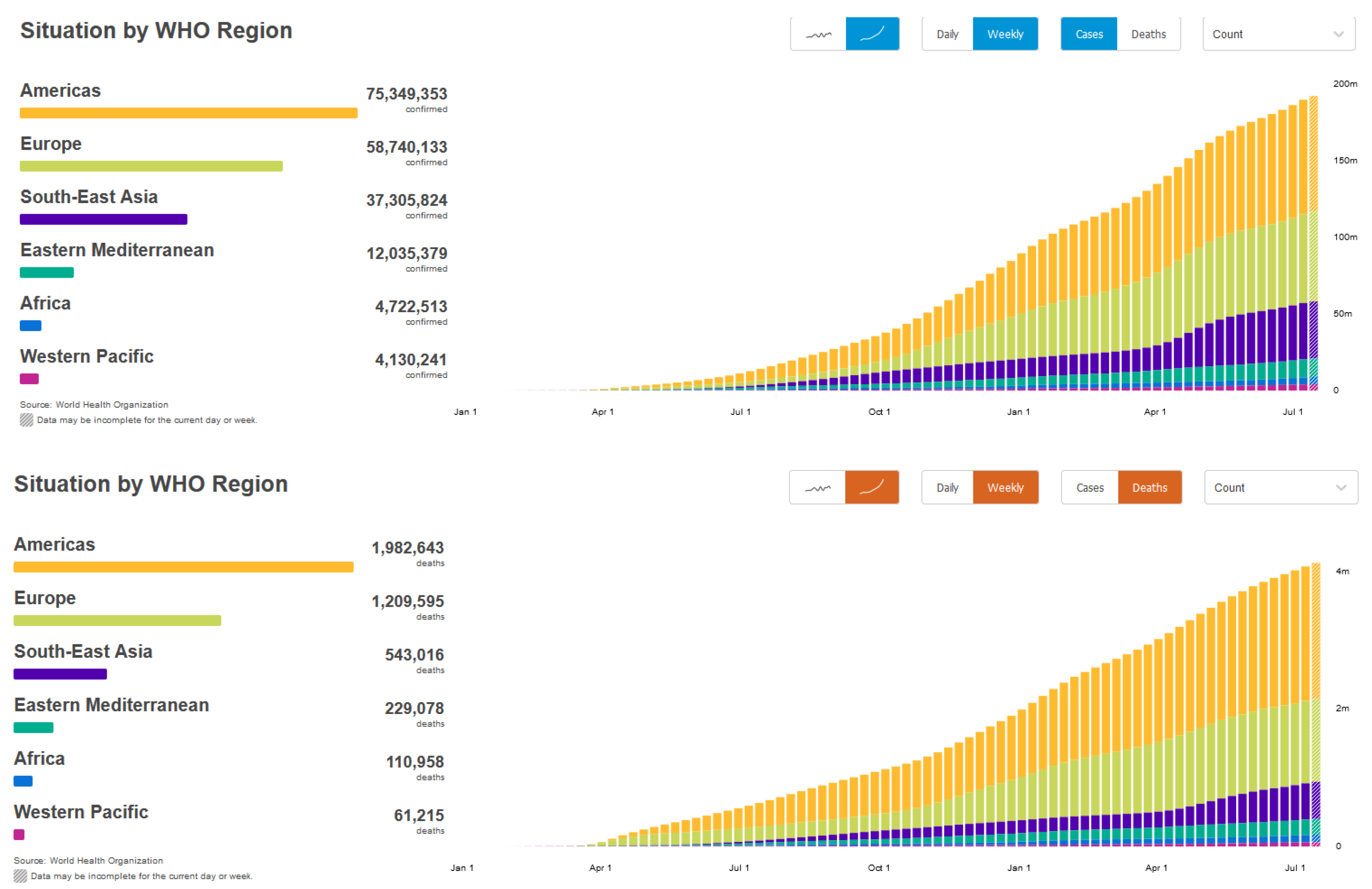
- WHO Coronavirus(COVID-19) Dashboard. 2021. Available online: https://covid19.who.int/ (accessed on 9 November 2021).
- Kantamneni, N. The impact of the COVID-19 pandemic on marginalized populations in the United States: A research agenda. In Elsevier Public Health Emergency Collection; Elsevier: Amsterdam, The Netherlands, 2020. [Google Scholar]
- University of Illinois Chicago. COVID-19: The Disproportionate Impact on Marginalized Populations. 2020. Available online: https://socialwork.uic.edu/news-stories/COVID-19-disproportionate-impact-marginalized-populations/ (accessed on 9 November 2021).
- CDC. COVID-19 Risks and Vaccine Information for Older Adults. 2021. Available online: https://www.cdc.gov/aging/covid19/covid19-older-adults.html (accessed on 9 November 2021).
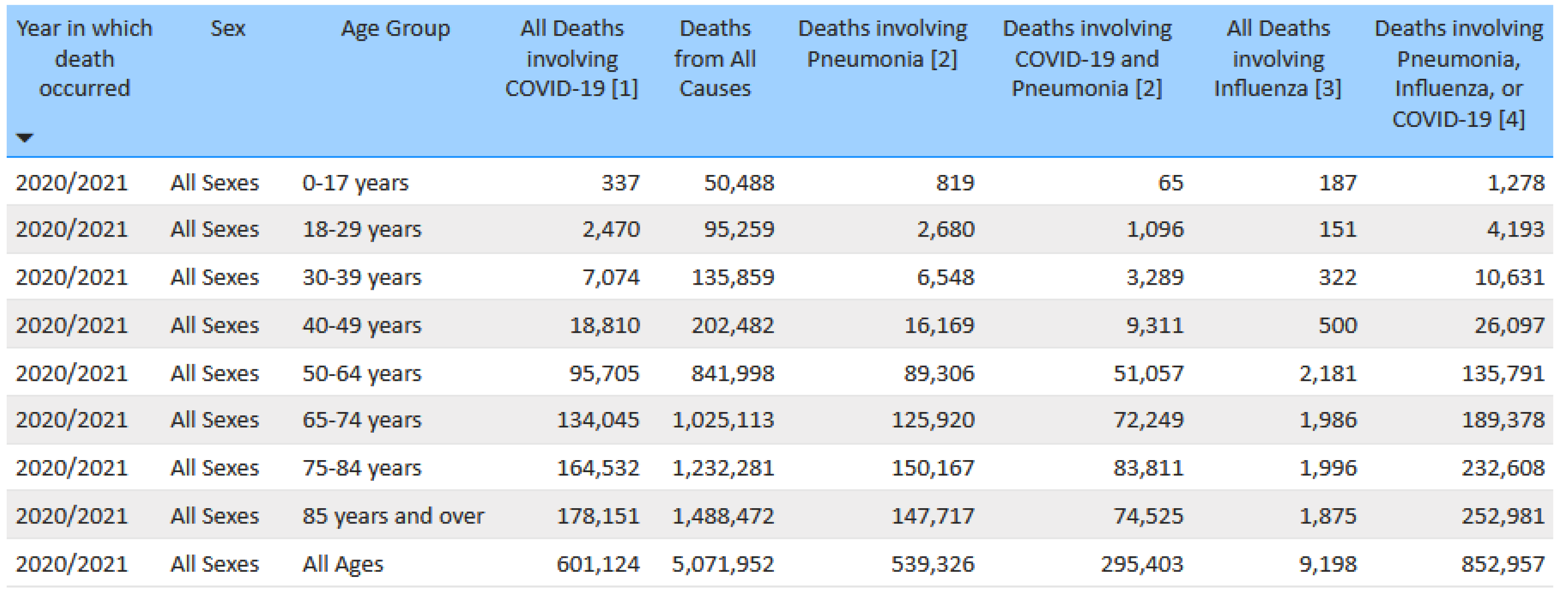
- CDC. Deaths Involving Coronavirus Disease 2019. 2021. Available online: https://www.cdc.gov/nchs/nvss/vsrr/covid_weekly/index.htm (accessed on 9 November 2021).
- Foundation, K.F. Population Distribution by Age. 2019. Available online: https://www.kff.org/other/state-indicator/distribution-by-age/?currentTimeframe=0&sortModel (accessed on 9 November 2021).
- Mueller, A.L.; McNamara, M.S.; Sinclair, D.A. Why does COVID-19 disproportionately affect older people? Aging 2020, 12, 9959–9981. [Google Scholar] [CrossRef] [PubMed]
- Gammaitoni, L.; Nucci, M.C. Using a Mathematical Model to Evaluate the Efficacy of TB Control Measures. Emerg. Infect. Dis. 1997, 3, 335–342. [Google Scholar] [CrossRef] [PubMed]
- Wells, W. On air-borne infection: Study II. Droplets and droplet Nuclei. Am. J. Epidemiol. 1934, 20, 611–618. [Google Scholar] [CrossRef]
- Riley, E.C.; Murphy, G.; Riley, R.L. Airborne spread of measles in a suburban elementary school. Am. J. Epidemiol. 1978, 107, 421–432. [Google Scholar] [CrossRef] [PubMed]
- da Silva, A. Modeling COVID-19 in Cape Verde Islands—An application of SIR Model. Comput. Math. Biophys. 2021, 9, 1–13. [Google Scholar] [CrossRef]
- Sowole, S.O.; Ibrahim, A.A.; Sangare, D.; Ibrahim, I.O.; Johnson, F.I. Understanding the Early Evolution of COVID-19 Disease Spread using Mathematical Mathematical Model and Machine Learning Approaches. Glob. J. Sci. Front. Res. F Math. Decis. Sci. 2020, 19–36. [Google Scholar] [CrossRef]
- Noakes, C.J.; Beggs, C.B.; Sleigh, P.A.; Kerr, K.G. Modelling the transmission of airborne infections in enclosed spaces. Epidemiol. Infect. 2006, 134, 1082–1091. [Google Scholar] [CrossRef] [PubMed]
- Feng, Z.; Towers, S. Social contact patterns and control strategies for influenza in the elderly. Math. Biosci. 2012, 240, 241–249. [Google Scholar]
- Diekmann, O.; Heesterbeek, J.A.; Roberts, M.G. The construction of next-generation matrices for compartmental epidemic models. J. R. Soc. Interface 2009, 7, 873–885. [Google Scholar] [CrossRef] [PubMed] [Green Version]
- Rudnick, S.; Milton, D. Risk of airborne infection transmission estimated from carbon dioxide concentration. Natl. Libr. Med. 2003, 13, 237–245. [Google Scholar]
- The President and Fellows of Harvard College. COVID-19 Basics; Harvard Health Publishing: Boston, MA, USA, 2021; Available online: https://www.health.harvard.edu/diseases-and-conditions/covid-19-basics (accessed on 9 November 2021).
- Maragakis, L. Coronavirus Diagnosis: What Should I Expect. 2021. Available online: https://www.hopkinsmedicine.org/health/conditions-and-diseases/coronavirus/diagnosed-with-COVID-19-what-to-expect (accessed on 9 November 2021).
- David, C.D., III; David, Z. Mild to Moderate COVID-19—Discharge. 2021. Available online: https://medlineplus.gov/ency/patientinstructions/000976.htm (accessed on 9 November 2021).
- George, N.; Tyagi, N.K.; Prasad, J.B. COVID-19 pandemic and its average recovery time in Indian states. Clin. Epidemiol. Glob. Health 2021, 11, 100740. [Google Scholar] [CrossRef] [PubMed]
- Johansson, M.A.; Quelacy, T.M.; Kada, S.; Prasad, P.V.; Steele, M.; Brooks, J.T.; Slayton, R.B.; Biggerstaff, M.; Butler, J.C. SARS-CoV-2 Transmission From People Without COVID-19 Symptoms. JAMA Netw. 2021, 4, e2035057. [Google Scholar] [CrossRef] [PubMed]
- Mossong, J.; Hens, N.; Jit, M.; Beutels, P.; Auranen, K.; Mikolajczyk, R.; Massari, M.; Salmaso, S.; Tomba, G.S.; Wallinga, J.; et al. Social Contacts and Mixing Patterns Relevant to the Spread of Infectious Diseases. PLoS Med. 2008, 5, e74. [Google Scholar] [CrossRef] [PubMed]
- Liu, Y.; Rocklöv, J. The reproductive number of the Delta variant of SARS-CoV-2 is far higher compared to the ancestral SARS-CoV-2 virus. Int. Soc. Travel Med. 2021, 28, taab124. [Google Scholar] [CrossRef] [PubMed]


Publisher’s Note: MDPI stays neutral with regard to jurisdictional claims in published maps and institutional affiliations. |
© 2021 by the authors. Licensee MDPI, Basel, Switzerland. This article is an open access article distributed under the terms and conditions of the Creative Commons Attribution (CC BY) license (https://creativecommons.org/licenses/by/4.0/).
Share and Cite
Gaddis, M.D.; Manoranjan, V.S. Modeling the Spread of COVID-19 in Enclosed Spaces. Math. Comput. Appl. 2021, 26, 79. https://doi.org/10.3390/mca26040079
Gaddis MD, Manoranjan VS. Modeling the Spread of COVID-19 in Enclosed Spaces. Mathematical and Computational Applications. 2021; 26(4):79. https://doi.org/10.3390/mca26040079
Chicago/Turabian StyleGaddis, Matthew David, and Valipuram S. Manoranjan. 2021. "Modeling the Spread of COVID-19 in Enclosed Spaces" Mathematical and Computational Applications 26, no. 4: 79. https://doi.org/10.3390/mca26040079