Article

ROM-Based Inexact Subdivision Methods for PDE-Constrained Multiobjective Optimization

1
Department of Mathematics and Statistics, University of Konstanz, 78457 Konstanz, Germany
2
Faculty for Computer Science, Electrical Engineering and Mathematics, Paderborn University, 33098 Paderborn, Germany
*
Author to whom correspondence should be addressed.
These authors contributed equally to this work.
Math. Comput. Appl. 2021, 26(2), 32; https://doi.org/10.3390/mca26020032
Submission received: 25 February 2021 / Revised: 7 April 2021 / Accepted: 13 April 2021 / Published: 15 April 2021
(This article belongs to the Special Issue Set Oriented Numerics 2022)

Abstract

:
The goal in multiobjective optimization is to determine the so-called Pareto set. Our optimization problem is governed by a parameter-dependent semi-linear elliptic partial differential equation (PDE). To solve it, we use a gradient-based set-oriented numerical method. The numerical solution of the PDE by standard discretization methods usually leads to high computational effort. To overcome this difficulty, reduced-order modeling (ROM) is developed utilizing the reduced basis method. These model simplifications cause inexactness in the gradients. For that reason, an additional descent condition is proposed. Applying a modified subdivision algorithm, numerical experiments illustrate the efficiency of our solution approach.

1. Introduction

Multiobjective optimization plays an important role in many applications, e.g., in industry, medicine, or engineering. One of the mentioned examples is the minimization of costs with simultaneous quality optimization in production or the minimization of CO2 emission in energy generation and simultaneous cost minimization. These problems lead to multiobjective optimization problems (MOPs), where we want to achieve an optimal compromise with respect to all given objectives at the same time. Normally, the different objectives are contradictory such that there exists an infinite number of optimal compromises. The set of these compromises is called the Pareto set. The goal is to approximate the Pareto set in an efficient way, which turns out to be more expensive than solving a single objective optimization problem.
As multiobjective optimization problems are of great importance, there exist several algorithms to solve them. Among the most popular methods are scalarization methods, which transform MOPs into scalar problems. For example, in the weighted sum method [1,2,3,4], convex combinations of the original objectives are optimized. Another popular approach is to use non-deterministic methods like evolutionary algorithms, cf., e.g., [5]. Furthermore, as multiobjective problems are generalizations of scalar problems, some solution methods can be generalized from the scalar to the multiobjective case [6,7,8].
In addition to the classical methods above, there are set-based strategies for the solution of MOPs. Continuation methods [9,10,11] use the fact that the Pareto set is typically (the projection of) a smooth manifold. Subdivision methods [12,13,14,15] use tools from the area of dynamical systems to generate a covering of the Pareto set via hypercubes. However, especially when the objective functions and their gradients are expensive to evaluate, e.g., as an underlying PDE has to be solved for every evaluation, the computational time of these methods can quickly become very large. In the presence of PDE constraints, surrogate models offer a promising tool to reduce the computational effort significantly [16]. Examples are dimensional reduction techniques such as the Reduced Basis (RB) Method [17,18]. In an offline phase, a low-dimensional surrogate model of the PDE is constructed by using, e.g., the greedy algorithm, cf. [17]. In the online phase, only the RB model is used to solve the PDE, which saves a lot of computing time.
In this article, we combine an extension of the set-oriented method presented in [12] based on inexact gradient evaluations of the objective functions with an RB approach and a discrete empirical interpolation method (DEIM) [19,20] for semi-linear elliptic PDEs. In order to deal with the inexactness introduced by the surrogate model, we combine the first-order optimality conditions for multiobjective optimization problems with error estimates for the RB-DEIM method and derive an additional condition for the descent direction [9] to get a tight superset of the Pareto set. This approach allows us to better control the quality of the result by controlling the errors for the objective functions independently. In order to obtain an even tighter superset of the Pareto set, we update these error estimates in our subdivision algorithm after each iteration step.
The article is organized as follows. In Section 2, we recall the basic concepts of multiobjective optimization problems and review results on descent directions with exact and inexact gradients. Furthermore, we develop a set-oriented method to solve these problems, where only inexact gradient information is utilized. In Section 3, the PDE-constrained multiobjective optimization problem and the underlying semi-linear PDE are introduced. Subsequently, we show how reduced-order modeling can be applied efficiently. In Section 4, numerical results concerning both the subdivision and the modified algorithm are presented. Finally, we give a conclusion and discuss possible future work in Section 5.

2. A Set-Oriented Method for Multiobjective Optimization with Inexact Objective Gradients

In this section, we briefly recall the basic concepts of multiobjective optimization. Furthermore, we develop a set-oriented method to solve these problems, where only inexact gradient information is utilized.

2.1. Multiobjective Optimization

Let μ a , μ b R m with μ a μ b be arbitrary. We define the convex and compact parameter set P ad = [ μ a , μ b ] R m . Now, the goal is to solve the constrained multiobjective optimization problem
min J ^ ( μ ) subject to ( s . t . ) μ P ad
with a given objective J ^ = ( J ^ 1 , , J ^ k ) : P ad R k and k > 1 .
Compared to scalar optimization, we do not have a natural total order of R k for k > 1 . Therefore, we cannot expect that there is a single point in P ad that minimizes all objectives J ^ i simultaneously. For this reason, we make use of the following definition.
Definition 1.
(a)
A point μ ¯ P ad is called (globally) Pareto optimal, if there is no μ P ad satisfying J ^ ( μ ) J ^ ( μ ¯ ) . In that case we call μ ¯ a Pareto point.
(b)
The set of all Pareto points in P ad is called Pareto set and is denoted by
P = μ P ad | μ   i s   P a r e t o   o p t i m a l .
(c)
The image J ^ ( P ) R k of the Pareto set under J ^ is called the Pareto front.
If J ^ is continuously differentiable on an open set containing P ad , then there exists a first-order necessary condition for Pareto optimality. To formulate this condition, we define the convex, closed, and bounded set
k = α R k | α i 0 and i = 1 k α i = 1 .
Further, the row vector
J ^ i ( μ ) = J ^ i μ j ( μ ) 1 j m R 1 × m
stands for the gradient of the i-th objective J ^ i with i { 1 , , k } .
Definition 2.
If for a given μ ¯ P ad there exists an α ¯ = ( α ¯ i ) 1 i k k with
i = 1 k α ¯ i J ^ i ( μ ¯ ) ( μ μ ¯ ) = ( μ μ ¯ ) D J ^ ( μ ¯ ) α ¯ 0 for all μ P ad
then we call μ ¯ Pareto critical, where
D J ^ ( μ ) = J ^ 1 ( μ ¯ ) J ^ k ( μ ) R k × m
denotes the Jacobi matrix of J ^ at μ. The set of all Pareto critical points is called the Pareto critical set, denoted by P c .
Now, we recall the first-order necessary optimality conditions for (1).
Theorem 1.
Let J ^ be continuously differentiable and μ ¯ P ad Pareto-optimal. Then, μ ¯ is Pareto-critical, i.e., it holds P P c . Condition (2) is called the Karush–Kuhn–Tucker (KKT) condition for multiobjective optimization problems.
Proof. 
The claim follows from ([1] Theorem 3.25) and the specific choice of P ad . □
Remark 1.
(a)
Let μ ¯ belong to the interior of P ad , i.e., μ ¯ int ( P ad ) = ( μ a , μ b ) . Then (2) is equivalent to
i = 1 k α ¯ i J ^ i ( μ ¯ ) = α D J ^ ( μ ) = 0 i n R 1 × m
or
D J ^ ( μ ) α = 0 i n R m = R m × 1 ;
see also in [21].
(b)
Throughout the paper, we only calculate the Pareto critical points in the interior of P ad and make use of (3). The idea is to choose P ad sufficiently large so that we get P c i n t ( P ad ) .
(c)
Due to Theorem 1, we have
P P c = μ P ad | α = α ( μ ) k : D J ^ ( μ ¯ ) α = 0 i n R m i n t ( P ad ) .
provided P c int ( P ad ) holds true. ◊

2.2. Descent Direction with Exact Gradients

Next, we introduce the notion of a descent direction for the vector valued objective function J ^ at a non-Pareto critical point μ P c . From now on, we assume that J ^ : P ad R k is continuously differentiable (on an open set containing P ad ).
Definition 3.
The vector v R m is a descent direction for J ^ in μ P ad , if we have
J ^ i ( μ ) v 0 f o r a l l i { 1 , , k }
and if there is at least one i { 1 , , k } with J ^ i ( μ ) v < 0 .
One way to compute a descent direction is to solve a constrained quadratic optimization problem in R k as shown in the following theorem. For a proof we refer to the work in [8]. A similar result was shown in [22].
Theorem 2.
For given μ int ( P ad ) let α ¯ = α ¯ ( μ ) k be a (global) solution of the convex constrained quadratic minimization problem
min 1 2 D J ^ ( μ ) α 2 2 s . t . α k .
Then, we have either D J ^ ( μ ) α ¯ = 0 or v = D J ^ ( μ ) α ¯ R m is a descent direction for J ^ in μ.
Combined with a backtracking Armijo line search, the descent direction from Theorem 2 can be used to construct the steepest descent method in Algorithm 1.
Algorithm 1: Steepest descent method.
Mca 26 00032 i001
Remark 2.
(a)
If Algorithm 1 terminates after a finite number l of iterations, then μ l is a Pareto critical point.
(b)
Assume that Algorithm 1 does not stop after a finite number of iterations. Then, every accumulation point μ ¯ of the sequence { μ l } l N generated by Algorithm 1 is a Pareto critical point. A proof based on ([7], Theorem 1) can be found in ([23] Theorem 5.2.5). ◊

2.3. Descent Direction with Inexact Gradients

Suppose that we have continuously differentiable approximations J ^ = ( J ^ i ) 1 i k of the objective function J ^ satisfying
max μ P ad J ^ i ( μ ) J ^ i ( μ ) 2 ε i for i { 1 , . . . , k } ,
for given tolerances ε i 0 . By P P ad we denote the Pareto set for J ^ and by P P ad the Pareto set for J ^ . If we write P c , we mean the Pareto-critical set for J ^ and P c is the Pareto-critical set for J ^ . Note that, in general, we have neither P P nor P P .
In this section, our goal is to compute an approximation of P based on the approximation J ^ of the objective function and the error bounds ε i . We begin by investigating the relationship between the KKT conditions of the original objective function and its approximation.
Lemma 1.
Let (5) be satisfied and μ ¯ int ( P ad ) be Pareto-critical for J ^ with the KKT-condition vector α ¯ k . Then, it holds that
D J ^ ( μ ¯ ) α ¯ 2 i = 1 k α ¯ i ε i = α ¯ , ε 2 ε
with ε = ( ε i ) 1 i k , where we set α ¯ , ε 2 = α ¯ ε .
Proof. 
From μ ¯ int ( P ad ) and Remark 1-a) we infer that D J ^ ( μ ¯ ) α ¯ = 0 holds. Therefore,
D J ^ ( μ ¯ ) α ¯ 2 = D J ^ ( μ ¯ ) α ¯ D J ^ ( μ ¯ ) α ¯ 2 = j = 1 k ( J ^ j ( μ ¯ ) J ^ j ( μ ¯ ) ) α ¯ j 2 j = 1 k J ^ j ( μ ¯ ) J ^ j ( μ ¯ ) 2 α ¯ j j = 1 k ε j α ¯ j = α ¯ , ε 2 ε
which gives the desired results. □
Based on estimate (6), we define two approximation sets for the Pareto-critical set P c of J ^ .
Definition 4.
Let us introduce the two sets
P 1 = μ int ( P ad ) | min α k D J ^ ( μ ) α 2 2 ε 2 P ad
and
P 2 = μ int ( P ad ) | min α k D J ^ ( μ ) α 2 2 α , ε 2 2 0 P ad .
Lemma 2.
It holds that
P c P 2 , P c P 2 a n d P 2 P 1 .
Proof. 
Let μ ¯ P c be a Pareto-critical point of J ^ , then there exists α ¯ k with D J ^ ( μ ¯ ) α ¯ = 0 . From Lemma 1, it follows that P c P 2 . Next, we assume that μ ¯ P c is a Pareto-critical point of J ^ , then there exists α ¯ k with D J ^ ( μ ¯ ) α ¯ = 0 . This implies
min α k D J ^ ( μ ¯ ) α 2 2 α , ε 2 D J ^ ( μ ¯ ) α ¯ 2 2 α ¯ , ε 2 2 = α ¯ , ε 2 0 .
Therefore, we have μ ¯ P 2 . Let μ ¯ P 2 . Then, there exists α ¯ k with
D J ^ ( μ ¯ ) α ¯ 2 2 α ¯ , ε 2 2 0 .
Thus, we get D J ^ ( μ ¯ ) α ¯ 2 2 α ¯ , ε 2 2 ε 2 which implies P 2 P 1 . □
Our goal is to compute the set P 2 l via a descent method like Algorithm 1. To this end, the following theorem presents a modified version of the descent direction (4), which additionally takes the error bounds ε i into account.
Theorem 3.
Let ε = ( ε j ) 1 j k with ε 0 and μ int ( P ad ) be given. Assume that α ε is a minimizer of the quadratic problem
min α k D J ^ ( μ ) α 2 2 α , ε 2 2 .
Then, we have that μ P 2 or v ε = D J ^ ( μ ) α ε R m is a descent direction for J ^ in μ.
Proof. 
The Lagrange functions for (7) is given as
L : R k × R × R k R , ( α , λ , ϱ ) D J ^ ( μ ) α 2 2 α , ϵ 2 2 + λ 1 j = 1 k α j j = 1 k ϱ j α j .
As α ε is a minimizer of (7), we get Lagrangian multipliers λ R and ϱ R 0 k with
2 D J ^ ( μ ) D J ^ ( μ ) α ε 2 ε ε , α ε 2 + λ ( 1 , . . . , 1 ) ϱ = 0 , ϱ i 0 and ( α ε ) i ϱ i = 0 .
If we multiply (8) with α ε from the left, we get
2 α ε D J ^ ( μ ) D J ^ ( μ ) α ε 2 ε , α ε 2 2 λ i = 1 m ( α ε ) i ( α ε ) i ϱ i = 0
which implies
λ = 2 D J ^ ( μ ) α ε 2 2 α ε , ε 2 2 .
First case: λ 0 , then μ P 2 holds and we are done.
Second case: λ > 0 , then μ P 2 holds. In this case, we show that v ε = D J ^ ( μ ) α ε is a descent direction in μ for every objective function J ^ j with j = 1 , . . . , k :
Define
K ( μ ) = D J ^ ( μ ) α | α R k , α i 0 and i = 1 k α i = 1 .
If we can show that w v ε < 0 holds for every w K , we know that v ε is a descent direction for every objective function J i in μ .
Choose w K ( μ ) . Then, there exists an α w k with w = D J ^ ( μ ) α w , and using (8) we obtain
w v ε = D J ^ ( μ ) α w v ε = α w D J ^ ( μ ) D J ^ ( μ ) α ε = α w ε ε , α ε 2 + 1 2 λ ( 1 , . . . , 1 ) + 1 2 ϱ = α w , ε 2 α ε , ε 2 + 1 2 λ + 1 2 α w , ϱ 2 1 2 λ + α w , ϱ 2 λ 2 < 0 .
Therefore, v ε is a descent direction in μ for every objective function J ^ j , j = 1 , . . . , k . □
The descent direction v ε from the previous theorem will be referred to as the modified descent direction. Based on this direction, we can now construct a descent method for the computation of P 2 l , which is shown in Algorithm 2.
Algorithm 2: Descent method with inexact gradients.
Mca 26 00032 i002
Remark 3.
(a)
If Algorithm 2 terminates after l iteration steps, then μ l is contained in P 2 .
(b)
Assume that Algorithm 2 does not terminate after a finite number of iteration steps. Then, every accumulation point μ ¯ of the sequence { μ l } l N generated by Algorithm 2 is in the set P 2 . A proof based on ([7] Theorem 1) can be found in ([23] Theorem 5.3.5).
(c)
Note that the tolerance ε is constant for all l throughout Algorithm 2. In Section 2.5, we will adapt ε in each iteration. ◊

2.4. Subdivision Algorithm

As mentioned in the introduction, there exist set-based solution methods for MOPs which globally approximate the Pareto set via sets (instead of a finite number of points). Here, we will consider the subdivision algorithm [12,13,15], which computes an approximation of the Pareto set as a covering of hypercubes (or boxes). The idea is to start with a large box containing the Pareto set which is then iteratively subdivided into smaller boxes, while eliminating boxes that do not contain part of the Pareto set.
There are essentially two versions of the subdivision scheme: one is gradient free and, thus, is particularly useful in the case when the evaluation of gradients is computationally expensive. We refer to the work in [12], where this variant is utilized to numerically realize a reduced-order approach for a PDE-constrained multiobjective optimization problem. The other one is directly based on a dynamical systems approach and utilizes gradient information in a similar way to memetic algorithms, see in [8]. Here, we will generalize the latter to the case of inexact gradients.
For a stepsize t l > 0 , let us formulate a descent step of the optimization procedure by
μ l + 1 = a ( μ l ) = μ l + t l v l or μ l + 1 = a ε ( μ l ) = μ l + t l v ε l ,
where v l and v ε l are the descent directions given by Theorems 2 and 3, respectively, with the choice μ = μ l . Depending on the descent step that we use, we either want to compute the Pareto-critical set P c or the superset P 2 or P 1 of P c . As these sets are the sets of fixed points for their respective descent step, we want to find the subset A P int ( P ad ) satisfying a ( A P ) = A P or a ε ( A P ) = A P .
To generate the set A P , we will use a subdivision method. This method produces an outer approximation of the set A P in the form of a nested sequence of sets B 0 , B 1 , . . . P ( P ad ) , where P ( P ad ) denotes the power set of P ad and each B l is a subset of B l 1 in the sense that
B B l B B B l 1 B
holds and B l consists of finitely many subsets B covering A P for all l N . For each set B l , we define a diameter through diam ( B l ) = max B B l ( diam ( B ) ) . Algorithm 3 shows the classical subdivision method (based on Theorem 2) and our modified descent direction (based on Theorem 3).
Algorithm 3: Subdivision algorithm.
Mca 26 00032 i003
Remark 4.
In order to realize the subdivision algorithm numerically we choose a similar way as described in ([13] Remark 2.4). Instead of working explicitly with the centers and radii of the boxes, these are stored within a binary tree in the subdivision step, whereby the memory requirement is noticeably reduced. The selection step is implemented using a certain number of sample points in each box. These sample points are chosen either on an a priori defined grid or randomly within the boxes. Afterwards, a ( ε ) is evaluated in these points. For more details, we refer the reader to ([24] Section 5). ◊

2.5. Modified Subdivision Algorithm for Inexact Gradients

In Algorithm 2, we utilize the same error bounds ε = ε 1 , . . . , ε k with ε i 0 , i = 1 , . . . , k , in each iteration step l. Note that the larger the ε , the greater the difference between P c and P 2 or P 1 . In the algorithm, we produce an outer approximation of the set A P with a nested sequence of sets { B l } l N by
B ˜ l = B B l B P ad .
As it holds that B ˜ l P ad , we have
max J ^ i ( μ ) J ^ i ( μ ) 2 | μ B ˜ l max J ^ i ( μ ) J ^ i ( μ ) 2 | μ P ad for 1 i k .
Now we modify Algorithm 3 by utilizing the descent directions introduced in Theorem 3 and update ε after every iteration step l to generate a better approximation of the set A P . For updating ε , we use the formula
ε i l = sup J ^ i ( μ ) J ^ i ( μ ) 2 | μ B ˜ l for 1 i k
and set ε l = ( ε i l ) 1 i k . Due to the nested choice of the box coverings, we have ε i l + 1 ε i l for i = 1 , . . . , k and l N . In iteration step l, we generate the descent direction by computing
α ε l arg min D J ^ ( μ ) α 2 2 α , ε l 2 2 | α k .
Then, we set
v ε l = D J ^ ( μ ) α ε l and μ l + 1 = a ε l ( μ l ) = μ l + t l v ε l .
Typically, the set P 2 is far smaller then the admissible set P ad . Therefore, we expect that the error bounds in (9) become significantly smaller than the ones from (5). Therefore, we expect that we get better results with the modified function a ε l instead of a ε .

3. Multiobjective Optimization of a Semi-Linear Elliptic PDE

In this section, we introduce a multiobjective parameter optimization problem governed by a semi-linear elliptic PDE. Further, we show how reduced-order modeling can be applied efficiently.

3.1. Problem Formulation

Let Ω R d , d { 1 , 2 , 3 } , be a bounded domain with Lipschitz-continuous boundary Γ = Ω . Then, we consider the problem
min ( y , μ ) J ( y , μ ) = J 1 ( y , μ ) J k 1 ( y , μ ) J k ( y , μ ) = 1 2 Ω | y y 1 d | 2 d x Ω | y y k 1 d | 2 d x j = 1 m | μ j μ j d | 2
subject to the elliptic boundary value problem
c y + b y + d y 3 = f + i = 1 m μ i ξ i in Ω , c y n + y = g on Γ ,
where y V = H 1 ( Ω ) is the state variable and μ P ad = [ μ a , μ b ] the parameter. We suppose that g L r ( Γ ) with r > d 1 , ξ 1 , . . . , ξ m , f H = L 2 ( Ω ) , μ d = ( μ j d ) R m , and y 1 d , . . . , y k 1 d H . Moreover, b, c, and d are non-negative constants with c > 0 .
As Ω is a bounded connected open set with smooth boundary, it is known that V is a Hilbert space endowed with the inner product
φ , ψ V = Ω φ · ψ d x + Γ φ ψ d s for φ , ψ V
and the induced norm φ V = φ , φ V 1 / 2 for φ V , see ([25], p. 133) for instance.

3.2. The Parameter Dependent Semi-Linear Elliptic PDE

In this subsection, we study the state equation (11b). First, we define the nonlinear operator A : V V by
A ( y ) , φ V , V = Ω c y · φ + b y + d y 3 φ d x + Γ y φ d s for y , φ V .
Recall that d { 1 , 2 , 3 } implies V L 6 ( Ω ) , cf. ([26] Section 7). Therefore, the operator A is well defined. Moreover, for μ P ad the functional b μ V is given by
b μ , φ V , V = Ω f + i = 1 m μ i ξ i φ d x + Γ g φ d s for φ V .
Now, we define a weak solution to the state Equation (11b).
Definition 5.
A weak solution of (11b) is a function y V satisfying
A ( y ) , φ V , V = b μ , φ V , V f o r a l l φ V .
The following result is proved, e.g., in ([26] Section 4.2.3).
Proposition 1.
For a fixed parameter μ R m , there exists a unique solution y V to (11b). This solution is even continuous on Ω ¯ , and for a constant c it holds that
y V + y C ( Ω ¯ ) c g L r ( Γ ) + f + i = 1 m μ i ξ i H .
Remark 5.
We define the state space Y = V C ( Ω ¯ ) , which is a Banach space endowed with the natural norm
φ Y = φ V + φ C ( Ω ¯ ) f o r φ Y .
Motivated by Proposition 1 , we define the parameter-to-state mapping S : P ad Y as follows: For a given parameter μ P ad , the function y = S ( μ ) Y is the solution to (11b). It follows by standard arguments that S is continuously Fréchet-differentiable, see ([23] Sections 2 and 4). ◊

3.3. Reduced Formulation and Adjoint Approach

Utilizing the parameter-to-state mapping S , we define the reduced cost functional
J ^ ( μ ) = J ( S ( μ ) , μ ) = J ^ 1 ( μ ) J ^ k ( μ ) for μ P ad
with
J ^ i ( μ ) = 1 2 Ω | S ( μ ) ( x ) y i d ( x ) | 2 d x for 1 i k 1
and J ^ k ( μ ) = j = 1 m | μ j μ j d | 2 / 2 . Now, the reduced problem is given as
min J ^ ( μ ) s . t . μ P ad .
If μ ¯ P ad is a locally optimal solution to (13), then the pair ( S ( μ ¯ ) , μ ¯ ) is a locally optimal solution to (11). Conversely, if ( S ( μ ¯ ) , μ ¯ ) Y × P ad solves (11) locally, the parameter μ ¯ is a locally optimal solution to (13).
To apply the subdivision algorithm, the reduced objective function J ^ has to be Fréchet-differentiable, following immediately from the fact that the parameter-to-state operator S is Fréchet-differentiable, cf. Remark 5. The gradient of J ^ can be expressed by introducing adjoint variables. For that purpose, we define the operators B i : V × V V , 1 i k 1 , as
B i ( p , y ) , φ V , V = Ω c p · φ + b + 3 d y 2 p φ d x + Γ p φ d x G ( y y i d ) φ d x
for p , y , φ V . Next, we define adjoint variables.
Definition 6.
Let a parameter μ P ad be given and y ( μ ) = S ( μ ) Y . For every i { 1 , , k 1 } , we call the solution p i ( μ ) V to
B i ( p i ( μ ) , y ( μ ) ) , φ V , V = 0 f o r a l l φ V
the adjoint variable associated with the objective J ^ i .
Remark 6.
(a)
Notice that (14) is the weak formulation of the elliptic problem
c p i ( μ ) + b + 3 d y ( μ ) 2 p i ( μ ) = y ( μ ) y i d in Ω , c p i n ( μ ) + p i ( μ ) = 0 on Γ
for i = 1 , , k 1 .
(b)
Applying the Lax–Milgram lemma (see, e.g., ([26] Section 2)) one can show that (14) has a unique solution p i ( μ ) V for all μ P ad and i = 1 , , k 1 . ◊
Now, we can express the gradient of the reduced cost functional as follows:
J ^ i ( μ ) = Ω ξ 1 p i ( μ ) d x Ω ξ m p i ( μ ) d x for 1 i k 1 , J ^ k ( μ ) = μ μ d ,
where y ( μ ) Y and p i ( μ ) V , i { 1 , , k 1 } , solve (12) and (14), respectively.

3.4. Finite Element (FE) Galerkin Discretization

Let us briefly introduce a standard finite element (FE) method based on a triangulation of the spatial domain Ω . Here, we utilize piecewise linear FE ansatz functions φ 1 , , φ N V , which are linearly independent. We define the finite-dimensional subspace V N = span { φ 1 , . . . , φ N } V supplied with the same topology as in V.
Next, we replace (12) by a FE Galerkin scheme: For each μ P ad , the FE solution y N ( μ ) V N solves
A ( y N ( μ ) ) , φ i V , V = b μ , φ i V , V for i = 1 , , N .
It follows by the same arguments as for (12) that the FE problem (16) has a unique solution y N = y N ( μ ) for every μ P ad . Therefore, the parameter-to-state FE mapping S N : P ad V N , μ S N ( μ ) = y N ( μ ) is well defined. For y N V N there exist coefficients y i N , i = 1 , , N , satisfying
y N = i = 1 N y i N φ i for x Ω .
Inserting (17) into (16), we can express (16) as a nonlinear algebraic system. For that purpose, we introduce the N × N -matrices
K = Ω φ j · φ i d x , M = Ω φ j φ i d x , Q = Γ φ j φ i d s ,
the N-vectors
y N = y i N , F μ = Ω ( f + j = 1 m μ j ξ j φ i d x ) , G = Γ g φ i d s ,
and the nonlinearity function H : R N R N given as
H ( v ) = Ω j = 1 N v j φ j 3 φ i d x for v = v 1 , , v N R N .
Inserting (17) into (16), we end up with the following nonlinear system:
c K + b M + Q y N + d H ( y N ) = F μ + G R N .
Remark 7.
The difficulty of (18) lies in the fact that we cannot assemble H ( y N ) efficiently in terms of a matrix-vector multiplication. Therefore, we use mass lumping to compute H ( y N ) approximately. For an introduction into mass lumping see, e.g., ([27] Section 15) or ([28] Section 17.2). With that we can write (18) as a root finding problem of
c K + b M + Q y N + d M ˜ ( y N ) 3 = F μ + G R N
with ( y N ) 3 = ( ( y i N ) 3 ) 1 i N and the lumped mass matrix M ˜ defined by
M ˜ k j : = δ k j l = 1 N M k l .
Further details can be found in [23,29]. Let us refer to in [30], where mass lumping is utilized in optimal control. ◊
Now, the FE objectives are given as
J ^ i N ( μ ) = 1 2 Ω | S N ( μ ) y i d | 2 d x for i = 1 , . . . , k 1 , J ^ k N ( μ ) = j = 1 m | μ j μ j d | 2 .

3.5. Reduced-Order Modelling (ROM)

To generate the Pareto-critical set of the MOP (11), we need to evaluate the reduced objectives J ^ i , i = 1 , , k , and their gradients many times. Therefore, the state and adjoint equations have to be solved numerically very often. Therefore, the use of ROM is a suitable option. In this paper, we will use the Reduced Basis (RB) method. The main idea is to construct a low-dimensional (i.e., N ) subspace V of the FE space V N spanned by FE solutions of the state and adjoint equation for appropriately chosen parameters μ P ad . Here, this strategy is realized by greedy algorithms. We refer to the works in [17,18,31] for a general explanation and to ([23] Section 3.2) for our specific problem (11). This is an iterative procedure where in each iteration FE solutions of the state and adjoint equation at a specific parameter value are added to the basis. An essential ingredient of greedy algorithms is the choice of an error indicator η ( μ ) . Here, we use the maximal true error between the FE and the ROM gradients, i.e., we set
η ( μ ) : = max 1 i k J ^ i N ( μ ) J ^ i ( μ ) 2 .
Our subdivision scheme is based on gradient information. To be able to generate P 1 or P 2 for the approximation of P , we have to ensure that the approximated objective function J ^ based on the ROM model satisfies the inequality in (5). The idea is to generate a new basis element in every step until the maximum error η ( μ ) on a discrete training set S t r a i n , which approximates P ad good enough, is smaller than a tolerance ε t o l . For more details, see Algorithm 4.
Algorithm 4: Greedy algorithm.
Mca 26 00032 i004
As V is a subset of V, we endow V with the V-topology. Due to ψ j V N ( 1 j ), there exists a coefficient matrix Ψ R N × such that
ψ j ( x ) = i = 1 N Ψ i j φ i ( x ) for x Ω .
Now, we replace (16) by an RB Galerkin scheme: For each μ P ad , the RB solution y ( μ ) V solves
A ( y ( μ ) ) , ψ i V , V = b μ , ψ i V , V for i = 1 , , .
We suppose that (22) has a unique solution y = y ( μ ) for every μ P ad . Therefore, the parameter-to-state RB mapping S : P ad V , μ S ( μ ) = y ( μ ) is well defined.
Inserting (21) and y ( μ ) = i = 1 N y i ( μ ) ψ i into (22), we derive the nonlinear algebraic system (cf. (18))
c K + b M + Q + d Ψ H Ψ y = F μ + G R l ( N )
with the × matrices K = Ψ K Ψ , M = Ψ M Ψ , and Q = Ψ Q Ψ and the -vectors F μ = Ψ F μ and G = Ψ G .
Remark 8.
As mentioned in Remark 7, we apply mass lumping to evaluate the nonlinear function H more efficiently. With that we can write (23) as a root finding problem of
c K + b M + Q y + d M ˜ Ψ y 3 = F μ + G R l ( N )
with ( Ψ y ) 3 = ( ( ( Ψ y ) i 3 ) ) 1 i N and the × N matrix M ˜ = Ψ M ˜ . However, in the RB Galerkin scheme the evaluation of the nonlinearity is still as costly as in the FE case. Here, discrete empirical interpolation (DEIM) is applied, cf. [19,20]. We skip the detailed description here and refer the reader to ([23] Section 3.2). ◊

3.6. Convergence Analysis

We prove the convergence of the RB solution with mass lumping to the weak solution of the state and adjoint equation.
Remark 9.
As the FE space is a finite dimensional space, the error for the state and adjoint equation converges for increasing dimension of the RB space to zero. Therefore, the RB solution converges for increasing accuracy in the Greedy algorithm to the FE solution. We skip a detailed description of the proof here and refer the reader to ([23], Section 3.2). ◊
Theorem 4.
Let ( S j ) j P ad with S j S j + 1 be a growing sequence of training sets and choose a monotone sequence ( ε j ) j R > 0 satisfying
ε j 0 for j and ε j ε j + 1 .
Then, we get
lim sup j y ( μ ) y ( μ ) V | μ P ad = 0 , lim sup j p ( μ ) p ( μ ) V | μ P ad = 0 .
Proof. 
Let μ P ad be an arbitrary parameter. It holds that
y ( μ ) y ( μ ) V y ( μ ) y N ( μ ) V + y N ( μ ) y ( μ ) V
with N > . From Theorem A1 (see Appendix A), we infer that the first summand converges to zero for increasing N. For the second summand, we refer the reader to ([23] Section 3.2.5); in this section we proved the convergence of the RB solution to the FE solution. For the adjoint equation, we can do the same and the claim follows. □

4. Numerical Experiments

In this section, we use our algorithm to solve multiobjective optimization problems with PDE constraints and interpret the numerical results. All computations were executed on a computer with a 2.9 GHz Intel Core i7 CPU, 8 GB of RAM, and an Intel HD Graphic 4000 1536 MB GPU. The algorithms were implemented in Matlab R2017b. For the subdivision method, we used the implementation from https://math.uni-paderborn.de/en/ag/chair-of-applied-mathematics/research/software.
In this example, we will numerically investigate the application of the modified subdivision algorithm presented in Section 2.5 to the PDE-constrained multiobjective optimization problem using the RB-DEIM solver from Section 3.5. For the underlying PDE, we set d = 2 , Ω = ( 0 , 1 ) 2 with elements x = ( x 1 , x 2 ) , P ad = [ 2 , 2 ] 2 , and b = c = d = 1 ; the right-hand side f ( x ) = x 1 2 + x 2 2 4 + ( x 1 2 + x 2 2 ) 3 , m = 2 , ξ 1 ( x ) = 25 · 1 x 1 > 0.5 ( x ) , and ξ 2 ( x ) = 25 · 1 x 1 0.5 ( x ) ; and the boundary condition g ( x ) = 2 · 1 x 1 = 1 ( x ) + 2 · 1 x 2 = 1 ( x ) + x 1 2 + x 2 2 . This leads to the following PDE:
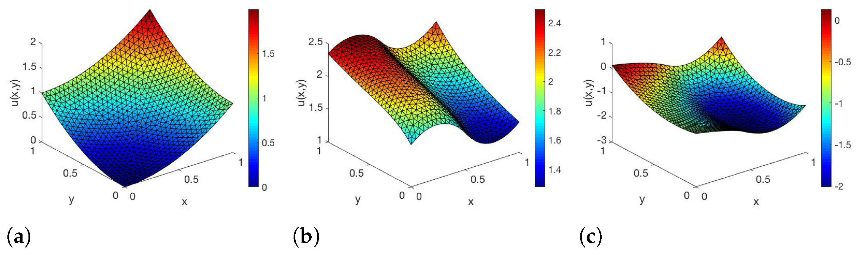
y + y + y 3 = f + μ 1 ξ 1 + μ 2 ξ 2 in Ω , y n + y = g on Ω .
In Figure 1, the corresponding solutions of the state equation are shown for three values of μ .
In [23], we have already observed that the error between the FE- and RB-DEIM-solution of the state and adjoint equation decreases if the FE grids get finer. We skip the detailed description here and refer the reader to ([23] Section 5).
Notice that y ( x ) = x 1 2 + x 2 2 solves (25) for μ = ( 0 , 0 ) . For the FE-solver, we used linear finite elements with H max = 0.04 and the finite elements have 762 degrees of freedom. We choose the following two objective functions:
J ^ 1 ( μ ) = 1 2 Ω | y ( μ ) y d | 2 d x , J ^ 2 ( μ ) = 1 2 j = 1 2 | μ j μ j d | 2
with μ d = ( 1 , 1 ) . For the desired state y d , we take the FE solution for μ = 0 , i.e., y d = y N ( 0 ) . Thus, y d = i = 1 N y i d φ i is a piecewise linear approximation of x 1 2 + x 2 2 . The associated FE objectives are now given as
J ^ 1 N ( μ ) = 1 2 y N ( μ ) y d M y N ( μ ) y d , J ^ 2 N ( μ ) = 1 2 j = 1 2 | μ j μ j d | 2
with y d = ( y i d ) 1 i N . The gradients are
J ^ 1 N ( μ ) = p N ( μ ) F ¯ 1 p N ( μ ) F ¯ 2 , J ^ 2 N ( μ ) = μ μ d
where p N ( μ ) = j = 1 N p j N ( μ ) φ j is the FE solution to (15), p N ( μ ) = ( p j N ( μ ) ) 1 j N and F ¯ i = ( Ω φ j ξ i d x ) 1 j N . The associated RB objective functions have the form
J ^ 1 ( μ ) = 1 2 y ( μ ) y d , M y ( μ ) y d , , J ^ 2 ( μ ) = 1 2 j = 1 m | μ j μ j d | 2
with y d , = Ψ y d . In [23], we have already observed good agreement between the approximated Pareto critical sets with the FE- and RB-DEIM-solver, if the error between the gradients is sufficiently small. However, we cannot always guarantee this agreement. Thus, we will instead use the supersets P 1 and P 2 from Section 2.3 for the approximation of P (and P c ), which is only based on the reduced objective function J ^ and the error bounds ε . To generate P 1 , we compute the steepest descent direction for all components of J ^ . Similar to Algorithm 1, we first calculate α k as solution of (4) for μ k . Then, the descent direction is v k : = D J ^ ( μ k ) α k . As a stopping condition, we choose σ = ε and set a ( μ k ) = μ k if it holds that
D J ^ ( μ k ) α k 2 = v k 2 < σ = ε .
To generate P 2 , we use Algorithm 2.
To save computational time during the modified subdivision algorithm, we calculate
max 1 i k J ^ i N ( μ ) J ^ i ( μ ) 2
before the algorithm starts (i.e., in an offline phase) on a training set P train , which approximates P ad and store these errors. During the subdivision algorithm, we use them to generate the new ε i + 1 l faster and without calculating the FE solution again.
To see a significant difference between the modified subdivision algorithm and the subdivision algorithm and P 2 and P 1 , we need to have a big error between the gradients. To achieve this, we choose a rough training set
S t r a i n = ( 2 + 0.51 k , 2 + 0.427 j ) | ( k , j ) { 0 , . . . , 7 } × { 0 , . . . , 9 }
with | S t r a i n | = 80 . For the Greedy algorithm, we choose the tolerance ε t o l = 0.06 and the true error η ( μ ) : = max 1 i k J ^ i N ( μ ) J ^ i ( μ ) 2 as error indicator, for the DEIM algorithm we choose the tolerance ε ¯ = 0.5 .
With these settings, we generate an RB-basis with six elements and a DEIM-basis with 18 elements. This leads to the following estimations for the gradients of J ^ N and J ^ :
max μ P ad J ^ 1 N ( μ ) J ^ 1 ( μ ) 2 max μ P train J ^ 1 N ( μ ) J ^ 1 ( μ ) 2 0.0491 = ε 1 , max μ P ad J ^ 2 N ( μ ) J ^ 2 ( μ ) 2 = max μ P ad J ^ 2 ( μ ) J ^ 2 ( μ ) 2 = 0 = ε 2 .
To generate these estimations, we chose a training set P train P ad with 3105 equally distributed test points and generate the error for these points. Thus, we have
ε 0 = 0.0491 0 .
Now, we test the subdivision and the modified subdivision algorithm with the following conditions. To compute the descent direction, we use the Matlab function fmincon and solve (4) or (7). The algorithm stops when the box size is small enough, which is after 25 iteration steps in our case. In every step, we halve the boxes. We choose five sample points in each box during the first five iteration steps, four sample points in the next five iteration steps, three sample points for the iteration steps ten to 14, two sample points for the next five steps, and one sample points for the last five iteration steps, see Remark 4. 
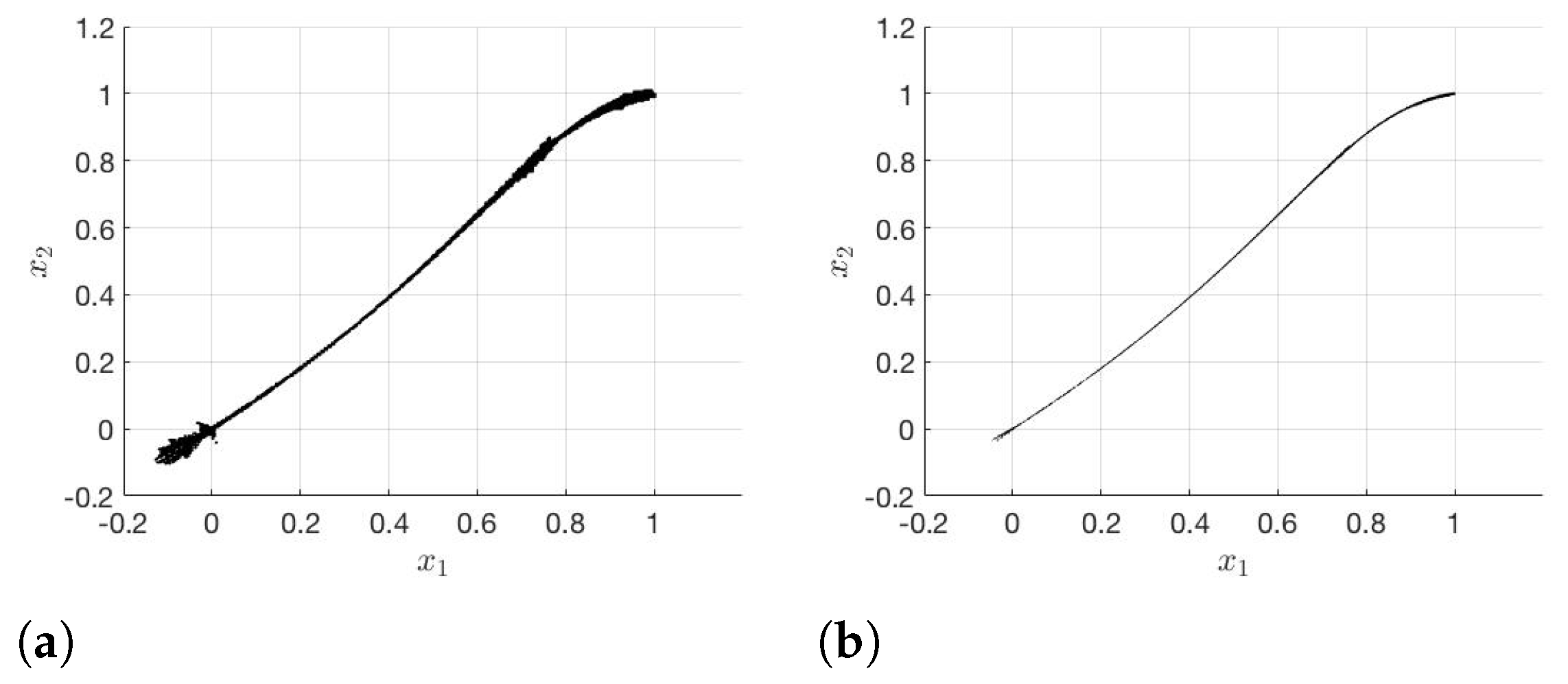
Figure 2 shows the generated approximated Pareto sets for the FE-solver after 20 and 25 iteration steps.
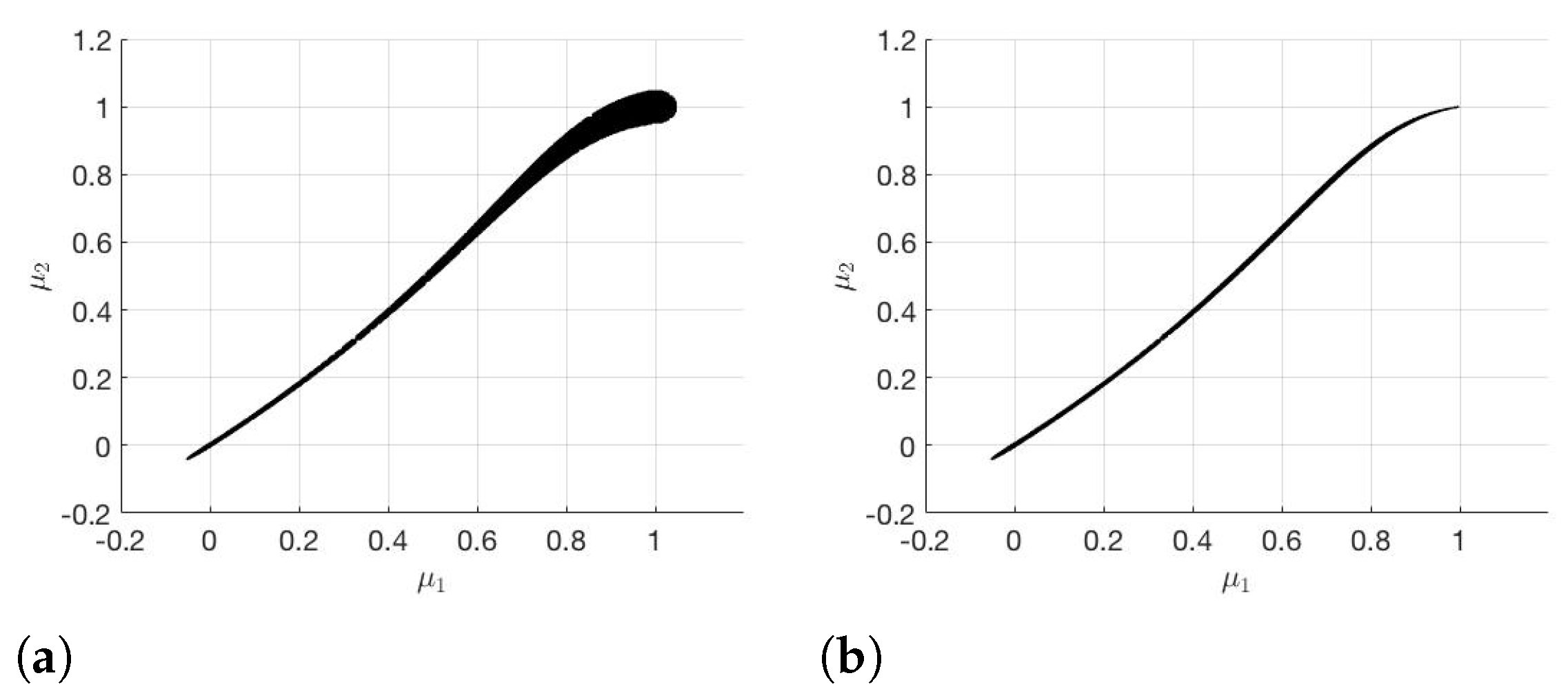
The results with the subdivision algorithm and RB-DEIM-solver are shown in Figure 3.
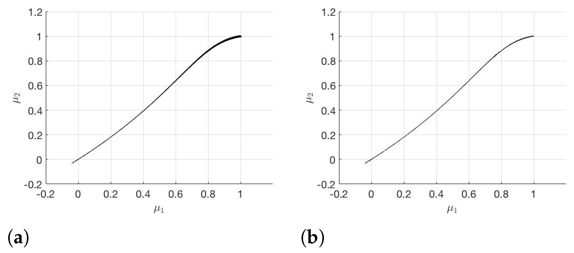
The modified subdivision algorithm and RB-DEIM-solver lead to the results plotted in Figure 4.
The runtime, number of boxes and number of function and gradient evaluations needed in iteration step 10, 15, 20, and 25 are shown in Table 1, Table 2, Table 3, Table 4 and Table 5. The total runtime and number of function and gradient evaluations needed for the different methods and the speed-up are shown in Table 6.
The Greedy algorithm and DEIM together take 14.06 s in the offline phase. To ensure the error ε (cf. (5)) for the gradients on the training set P train , it takes 151.13 s. It follows from Figure 3 and Figure 4 that P 2 is significantly smaller than P 1 for the subdivision algorithm as well as for the modified subdivision algorithm. Therefore, we have a much better approximation for P c if we choose P 2 instead of P 1 . If we compare the two different subdivision algorithms, we notice that with the modified subdivision algorithm we have a better approximation of P c than with the subdivision algorithm.
The reason for this is that in the modified subdivision algorithm we have a monotonically decreasing sequence
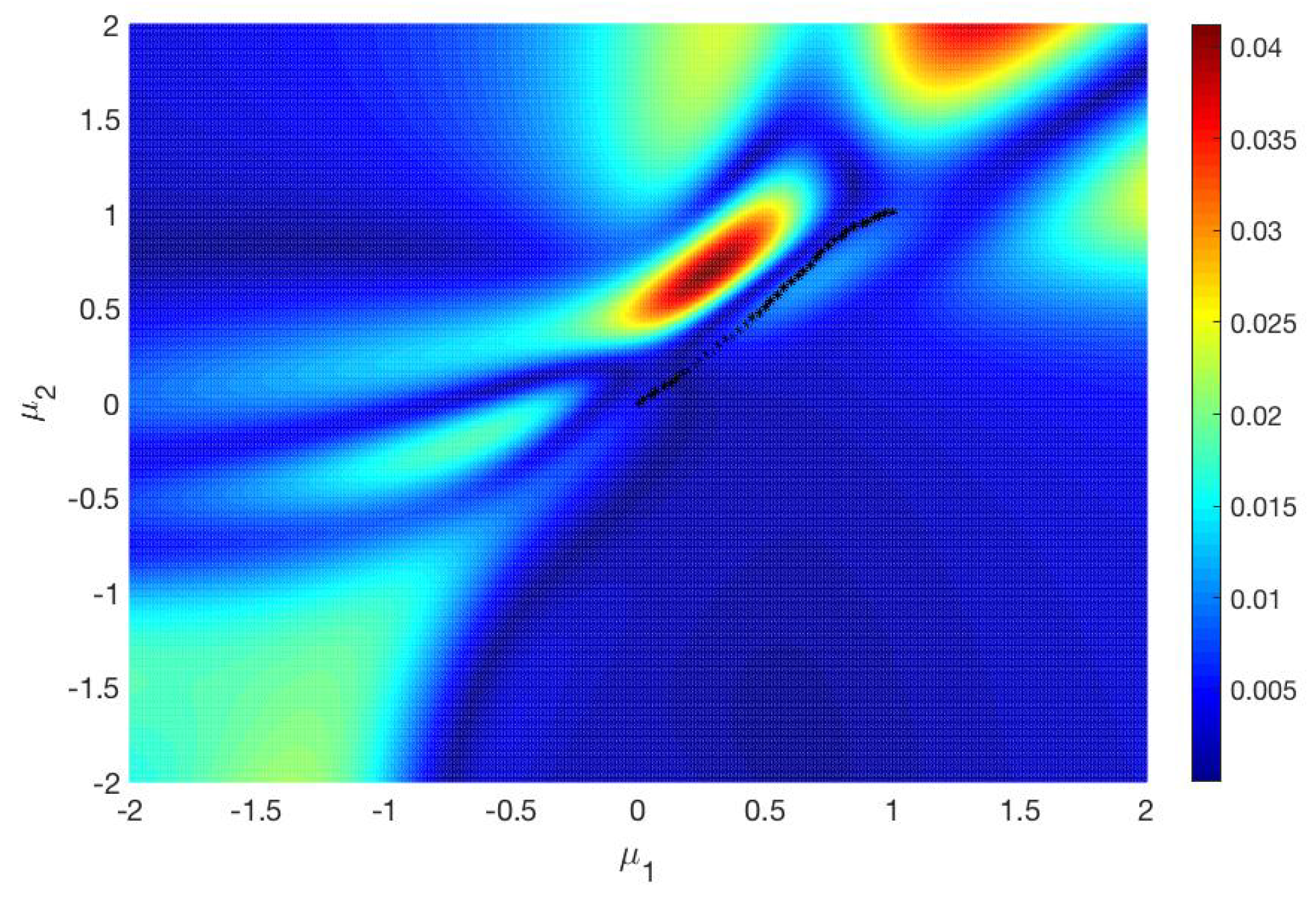
 ε l . In Figure 5, the error between J ^ 1 N and J ^ 1 is plotted on the parameter set P ad . The black markers are some points on the Pareto critical set P c . It turns out that the difference between the two gradients is significantly smaller near P c than in other regions of P ad . Due to this, in the modified subdivision algorithm, the sequence ε l decreases noticeably so that it is useful to update ε after each iteration step. As we have already mentioned, P 2 is a better approximation of P c . If P 2 is generated by the modified subdivision algorithm, the result is even better. Comparing Figure 2b and Figure 4b, there is no significant difference between the two sets. Therefore, the modified subdivision algorithm yields a good approximation P 2 for P c , although the error ε 1 is not small.
Regarding the computational time (cf. Table 1, Table 2, Table 3, Table 4, Table 5 and Table 6), we notice that in the first 20 iterations the four methods take almost the same time. In these iteration steps, the FE-solver takes between 19 and 30 times more time for one iteration step than the four RB-based methods. Only in the subsequent iteration steps a significant difference in the four RB-based methods appears. For these iteration steps, the FE-solver takes between 3.9 and 30.8 times as much time as one of the four methods for one iteration step. We notice that the computation of P 1 takes around two times as much time as the computation of P 2 with the subdivision algorithm. The main reason for this is the much larger number of function and gradient evaluations that we have for P 1 . This, in turn, can be attributed to the significantly larger number of boxes for P 1 . If we use the modified subdivision algorithm, the computation of P 2 takes slightly more time than the computation of P 1 . The main reason for this is again the larger number of function and gradient evaluations. Unlike the previous case, this can not be lead back to the number of boxes, but probably to the calculation of the modified descent method, which requires more function and gradient evaluations. Nevertheless, the difference in the computational time is marginal (a factor about 1.04 ) for the modified subdivision algorithm. For P 1 , we notice another behavior: Here, the generation of P 1 with the modified subdivision algorithm is 2 times faster than with the subdivision algorithm. This is mainly because of the larger number of function evalutions, which is due to the larger number of boxes. The FE-solver takes approximately 23.6 times as much time as the computation of P 1 and approximately 22.6 times as much as the time as the computation of P 2 with the modified subdivsion. This is another advantage of the modified subdivision algorithm. As we get a better approximation in this algorithm, we have fewer boxes in the iteration steps, and therefore we have a smaller number of function and gradient evaluations than we have for the subdivision algorithm. Finally, we see that the modified subdivision algorithm works better and faster than the subdivision algorithm. As P 2 is a tighter approximation of P c , it is better to generate P 2 rather than P 1 .

5. Conclusions

In this article, we present a way to solve multiobjective parameter optimization problems of semilinear elliptic PDEs by combining an RB approach and DEIM with the set-oriented method based on gradient evaluations. To deal with the error introduced by the surrogate model, we derived an additional condition for the descent direction, which allows us to consider the errors for the objective functions independently and derive a superset P 2 of the Pareto-critical set P c . To get an even tighter superset, we update these error bounds in our subdivision algorithm after each iteration step. To summarize the numerical results, we first investigated the influence of the error bounds for the gradients of the objective functions. By individually adapting the components of the error bounds, we obtained a tighter covering of the Pareto critical set. When we additionally adjusted the error bounds in each iteration step, the result became even tighter and almost coincided with the exact solution of the MOP (solution with the FE-solver and the steepest descent method). Furthermore, we compared the computational time for each method. The FE-solver needed between 11.9 times and 23.6 times more time than the four different RB-based methods we presented in this work. For future work, it could be interesting to improve the results in ([23] Section 3.2.4) and to develop an efficient a posteriori error estimator for the error in the objectives and their gradients, cf., e.g., [32,33,34]. These error bounds can then be used in a weak greedy algorithm and beyond that for the error bounds which are needed in the subdivision algorithm.

Author Contributions

The authors contributed equally to this work. All authors have read and agreed to the published version of the manuscript.

Funding

This research was funded partially by Deutsche Forschungsgemeinschaft grant number Priority Programme 1962.

Acknowledgments

The authors gratefully acknowledge partial support by the German DFG-Priority Program 1962. Furthermore, S. Banholzer acknowledges his partial funding by the Landesgraduiertenförderung of Baden-Württemberg.

Conflicts of Interest

The authors declare no conflict of interest.

Abbreviations

The following abbreviations are used in this manuscript:
MOPMultiobjective optimization problem
DEIMDiscrete Empirical Interpolation Method
FEFinite Element
GSGram–Schmidt
KKTKarush–Kuhn–Tucker
PDEPartial-differential equation
PODProper Orthogonal Decomposition
RBReduced Basis
ROMReduced Order Modeling

Appendix A. Mass Lumping

We follow the work in [35]. Let Ω R d , d { 1 , 2 , 3 } be an open, bounded Lipschitz domain, e.g., Ω = ( 0 , 1 ) d . We set H = L 2 ( Ω ) and V = H 1 ( Ω ) , where V is endowed with the inner product
φ , φ V = Ω φ · φ d x + Γ φ φ d s for φ , φ V
and its induced norm. Let T N denote an underlying triangulation of Ω and V ( T N ) = { z 1 , . . . , z N } denote the set of interior vertices of T N , and let V ( τ ) be the set of vertices belonging to τ T N and V N = span { φ 1 , . . , φ N } be the FE space generated by first order Lagrange elements. It holds that φ j ( z l ) = δ j l .
Define for z j V ( T N ) a lumped mass region Ω j by joining the centroids of the triangles, which have z j as a common vertex, to the midpoint of the edges, which have z j as a common extremity. We define the two sets
V N = v C ( Ω ¯ ) | v | τ j P 1   for   all   τ i T N V , H N = v L ( Ω ) | v = j = 1 N 1 Ω j v j , v j R H
and the operator
R N : C ( Ω ¯ ) H N , R N ( ω ) = j = 1 N 1 Ω j ω ( z j ) .
We consider the following semi-linear elliptic partial differential equation:
y + f ( y ) = h in Ω , y n + y = g on Γ = Ω .
A weak solution of (A1) is a function y Y = V L ( Ω ) such that
Ω y · φ + f ( y ) φ d x + Γ y φ d s = Ω h φ d x + Γ g φ d s for all φ V .
The function f is supposed to be sufficiently smooth, bounded, and measurable for a fixed y; monotonically increasing; and satisfies f 0 . Moreover, h H and g L r ( Γ ) with s > d 1 . Then, there exists a unique solution y Y of (A1), c.f. [26], for instance. This solution is even continuous, and for a constant c it holds that
y V + y C ( Ω ¯ ) c h H + g L r ( Γ ) .
The lumped mass finite element approximation of (A1) is to find y N V N such that
Ω y N · φ + f ( R N ( y N ) ) φ N d x + Γ y N φ d s = Ω h φ d x + Γ g φ d s
holds for all φ V N and for φ N = R N ( φ ) .
Remark A1.
For any v C ( Ω ¯ ) , it holds that R N ( v ) = j = 1 N 1 Ω j v ( z j ) . Therefore, R N ( v ) v for n , which implies
R N ( v ) v H 0 f o r n .
 ◊
Theorem A1.
Assume that y V and y N V N are solutions of (A2) and (A3), respectively. Then, it holds that
y y N V 0 f o r N .
Proof. 
Because y solves (A2), it holds that y C ( Ω ¯ ) . Let y p V N be the interpolation polynomial of y in V N . Then, it follows that R N ( y p ) = R N ( y ) . Utilizing (A3), we derive
Ω y N · y p Γ y N y p d s = Ω f ( R N ( y N ) ) R N ( y ) h y p d x Γ g y p d s .
Let ε > 0 be an arbitrary tolerance. For N large enough, we have y y p V < ε . Furthermore, we have R N ( y ) y H < ε and R N ( y p y N ) ( y p y N ) H < ε . From (A4), we conclude
y N y V 2 = Ω | ( y N y ) | 2 d x + Γ | y N y | 2 d s = Ω ( y N y ) · ( y p y ) + ( y N y ) · y N + ( y y N ) · y p d x + Γ ( y N y ) ( y p y ) + ( y N y ) y N + ( y y N ) y p d s = Ω ( y N y ) · ( y p y ) + ( y N y ) · y N + y · y p d x + Γ ( y N y ) ( y p y ) + ( y N y ) y N + y y p d s + Ω f ( R N ( y N ) ) R N ( y ) h y p d x Γ g y p d s .
Utilizing y y p V < ε , R N ( y ) y H < ε , and R N ( y p y N ) ( y p y N ) H < ε , it follows that
Ω ( f ( R N ( y N ) ) R N ( y ) ) d x = f ( R N ( y N ) ) , R N ( y ) H = f ( R N ( y N ) ) f ( R N ( y ) ) , R N ( y ) R N ( y N ) H + f ( R N ( y N ) ) , R N ( y N ) H + f ( R N ( y ) ) , R N ( y ) R N ( y N ) H f ( R N ( y N ) ) , R N ( y N ) H + f ( R N ( y ) ) , R N ( y ) R N ( y N ) H = f ( R N ( y ) ) , R N ( y y N ) ( y y N ) H + f ( y ) , y y N H + f ( R N ( y ) ) f ( y ) , ( y y N ) H + f ( R N ( y N ) ) , R N ( y N ) H c y y p H + R N ( y p y N ) ( y p y N ) H + f ( y ) , y y N H + c R N ( y ) y H y y N H + f ( R N ( y N ) ) , R N ( y N ) H c 2 ε + ε y y N H + f ( y ) , y y N H + f ( R N ( y N ) ) , R N ( y N ) H .
Inserting this estimation into the equality before thus gives
y y N V 2 ε y y N V 2 + y p y V 2 4 ε + y N , ( y N y ) H d + y p , y H d + y N y , y p y L 2 ( Γ ) + y N , y N y L 2 ( Γ ) + y p , y L 2 ( Γ ) y p , h H y p , g L 2 ( Γ ) + c ε + c ε y y N H + g , y y N L 2 ( Γ ) y , y y N L 2 ( Γ ) + h , y y N H y , ( y y N ) H d + f ( R N ( y N ) ) , R N ( y N ) H c ε y y N V 2 + ε 2 4 ε + c ε y N , y H d + y p , y H d + g , y y p L 2 ( Γ ) + h , y y p H + y N , y p y L 2 ( Γ ) y , ( y y N ) H d c ε + c ε y y N V 2
with H d = i = 1 d H . In the last inequality, we used the fact that y p y for N . Therefore, we get
y y N V 2 c 0 ε
and it follows y y N V 0 for N . □
Remark A2.
For y N V N and j = 1 , , N we find
Ω f ( R N ( y N ) ) R N ( φ j ) d x = i = 1 N Ω i f l = 1 N y l N 1 Ω l 1 Ω j d x = Ω j f l = 1 N y l N 1 Ω l d x = f ( y j N ) Ω j 1 Ω j d x = f ( y j N ) τ T N : z j V ( τ ) | τ | n + 1 = M ˜ j j f ( y j N ) .
For the last step we use
M ˜ j j = k = 1 N M j k = τ T N : z j V ( τ ) τ φ j d x = τ T N : z j V ( τ ) | τ | n + 1 .
A detailed proof for this equality can be found in ([36], Appendix A). ◊

References

  1. Ehrgott, M. Multicriteria Optimization; Springer: Berlin/Heidelberg, Germany, 2005. [Google Scholar]
  2. Iapichino, L.; Ulbrich, S.; Volkwein, S. Multiobjective PDE-constrained optimization using the reduced-basis method. Adv. Comput. Math. 2017, 43, 945–972. [Google Scholar] [CrossRef]
  3. Miettinen, K. Nonlinear Multiobjective Optimization; Kluwer Academic Publishers: Dordrecht, The Netherlands, 1999. [Google Scholar]
  4. Zadeh, L. Optimality and non-scalar-valued performance criteria. IEEE Trans. Autom. Control 1963, 8, 59–60. [Google Scholar] [CrossRef]
  5. Deb, K. Multi-Objective Optimization Using Evolutionary Algorithms; John Wiley & Sons, Inc.: Hoboken, NJ, USA, 2001. [Google Scholar]
  6. Fliege, J.; Graña Drummond, L.M.; Svaiter, B.F. Netwon’s Method for multiobjective optimization. SIAM J. Optim. 2008, 20, 602–626. [Google Scholar] [CrossRef] [Green Version]
  7. Fliege, J.; Svaiter, B.F. Steepest descent methods for multicriteria optimization. Math. Methods Oper. Res. 2000, 51, 479–494. [Google Scholar] [CrossRef]
  8. Schäffler, S.; Schultz, R.; Weinzierl, K. Stochastic method for the solution of unconstrained vector optimization problems. J. Optim. Theory Appl. 2002, 114, 209–222. [Google Scholar] [CrossRef]
  9. Banholzer, S.; Gebken, B.; Dellnitz, M.; Peitz, S.; Volkwein, S. ROM-based multiobjective optimization of elliptic PDEs via numerical continuation. arXiv 2019, arXiv:1906.09075v1. [Google Scholar]
  10. Hillermeier, C. Nonlinear Multiobjective Optimization: A Generalized Homotopy Approach; Birkhäuser: Cambridge, MA, USA, 2001. [Google Scholar]
  11. Schütze, O.; Dell’Aere, A.; Dellnitz, M. On continuation methods for the numerical treatment of multi-objective optimization problems. In Practical Approaches to Multi-Objective Optimization; Branke, J., Deb, K., Miettinen, K., Steuer, R.E., Eds.; Dagstuhl Seminar Proceedings: Dagstuhl, Deutschland, 2005. [Google Scholar]
  12. Beermann, D.; Dellnitz, M.; Peitz, S.; Volkwein, S. Set-oriented multiobjective optimal control of PDEs using proper orthogonal decomposition. In Reduced-Order Modeling (ROM) for Simulation and Optimization: Powerful Algorithms as Key Enablers for Scientific Computing; Springer International Publishing: Cham, Switzerland, 2018; pp. 47–72. [Google Scholar]
  13. Dellnitz, M.; Schütze, O.; Hestermeyer, T. Covering Pareto sets by multilevel subdivision techniques. J. Optim. Theory Appl. 2005, 124, 113–136. [Google Scholar] [CrossRef]
  14. Jahn, J. Multiobjective search algorithm with subdivision technique. Comput. Optim. Appl. 2006, 35, 161–175. [Google Scholar] [CrossRef]
  15. Schütze, O.; Witting, K.; Ober-Blöbaum, S.; Dellnitz, M. Set oriented methods for the numerical treatment of multiobjective optimization problems. In EVOLVE—A Bridge between Probability, Set Oriented Numerics and Evolutionary Computation; Tantar, E., Tantar, A.-A., Bouvry, P., Del Moral, P., Legrand, P., Coello Coello, C.A., Schütze, O., Eds.; Springer: Berlin/Heidelberg, Germany, 2013; Volume 447, pp. 187–219. [Google Scholar]
  16. Schilders, W.H.; Van der Vorst, H.A.; Rommes, J. Model Order Reduction; Springer: Berlin/Heidelberg, Germany, 2008. [Google Scholar]
  17. Hesthaven, J.S.; Rozza, G.; Stamm, B. Certified Reduced Basis Methods for Parametrized Partial Differential Equations; SpringerBriefs in Mathematics: Heidelberg, Germany, 2016. [Google Scholar]
  18. Patera, A.T.; Rozza, G. Reduced Basis Approximation and A Posteriori Error Estimation for Parametrized Partial Differential Equations. MIT Pappalardo Graduate Monographs in Mechanical Engineering: Cambridge, MA, USA, 2007. [Google Scholar]
  19. Chaturantabut, S.; Sorensen, D.C. Nonlinear model reduction via discrete empirical interpolation. SIAM J. Sci. Comput. 2010, 32, 2737–2764. [Google Scholar] [CrossRef]
  20. Chaturantabut, S.; Sorensen, D.C. A state space estimate for POD-DEIM nonlinear model reduction. SIAM J. Numer. Anal. 2012, 50, 46–63. [Google Scholar] [CrossRef]
  21. Gebken, B.; Peitz, S.; Dellnitz, M. A descent method for equality and inequality constrained multiobjective optimization problems. In Numerical and Evolutionary Optimization—NEO 2017; Trujillo, L., Schütze, O., Maldonado, Y., Valle, P., Eds.; Springer: Cham, Switzerland, 2017. [Google Scholar]
  22. Graña Drummond, L.M.; Svaiter, B.F. A steepest descent method for vector optimization. J. Comput. Appl. Math. 2005, 175, 395–414. [Google Scholar] [CrossRef] [Green Version]
  23. Reichle, L. Set-Oriented Multiobjective Optimal Control of Elliptic Non-Linear Partial Differential Equations Using POD Objectives and Gradient. Master’s Thesis, University of Konstanz, Konstanz, Germany, 2020. Available online: http://nbn-resolving.de/urn:nbn:de:bsz:352-2-1h6pp1cxptbap6 (accessed on 15 April 2021).
  24. Dellnitz, M.; Hohmann, A. A subdivision algorithm for the computation of unstable manifolds and global attractors. Numer. Math. 1997, 75, 293–316. [Google Scholar] [CrossRef]
  25. Dautray, R.; Lions, J.-L. Mathematical Analysis and Numerical Methods for Science and Technology. Volume 2: Functional and Variational Methods; Springer: Berlin/Heidelberg, Germany, 2000. [Google Scholar]
  26. Tröltzsch, F. Optimal Control of Partial Differential Equations: Theory, Methods and Applications; American Mathematical Society: Providence, RI, USA, 2010; Volume 112. [Google Scholar]
  27. Thomée, V. Galerkin Finite Element Methods for Parabolic Problems; Springer: Berlin/Heidelberg, Germany, 2006. [Google Scholar]
  28. Zienkiewicz, O.C.; Taylo, R.L. The Finite Element Method, 5th ed.; Butterworth-Hienemann: Oxford, UK, 2000; Volume 3. [Google Scholar]
  29. Brenner, S.; Scott, R. The Mathematical Theory of Finite Element Methods; Springer: Berlin/Heidelberg, Germany, 2008. [Google Scholar]
  30. Rösch, A.; Wachsmuth, G. Mass lumping for the optimal control of elliptic partial differential equations. SIAM J. Numer. Anal. 2017, 55, 1412–1436. [Google Scholar] [CrossRef]
  31. Quarteroni, A.; Manzoni, A.; Negri, F. Reduced Basis Methods for Partial Differential Equations; Springer: Berlin/Heidelberg, Germany, 2016. [Google Scholar]
  32. Grepl, M.A.; Maday, Y.; Nguyen, N.C.; Patera, A.T. Efficient reduced-basis treatment of nonaffine and nonlinear partial differential equations. ESAIM Math. Model. Numer. Anal. 2007, 41, 575–605. [Google Scholar] [CrossRef] [Green Version]
  33. Hinze, M.; Korolev, D. Reduced basis methods for quasilinear elliptic PDEs with applications to permanent magnet synchronous motors. arXiv 2020, arXiv:2002.04288. [Google Scholar]
  34. Rogg, S.; Trenz, S.; Volkwein, S. Trust-region POD using a-posteriori error estimation for semilinear parabolic optimal control problems. Konstanz. Schr. Math. 2017, 359. Available online: https://kops.uni-konstanz.de/handle/123456789/38240 (accessed on 15 April 2021).
  35. Zeng, J.; Yu, H. Error estimates of the lumped mass finite element method for semilinear elliptic problems. J. Comput. Appl. Math. 2012, 236, 993–2004. [Google Scholar] [CrossRef] [Green Version]
  36. Bernreuther, M. RB-Based PDE-Constrained Non-Smooth Optimization. Master’s Thesis, University of Konstanz, Konstanz, Germany, 2019. Available online: http://nbn-resolving.de/urn:nbn:de:bsz:352-2-t4k1djyj77yn3 (accessed on 15 April 2021).
Figure 1. FE solutions of (25) for parameters (a) μ = ( 0 , 0 ) , (b) μ = ( 0 , 1 ) and (c) μ = ( 1 , 0 ) .
Mca 26 00032 g001
Figure 2. Pareto-critical set P c in iteration step (a) 20 and (b) 25 for the FE-solver.
Mca 26 00032 g002
Figure 3. (a) P 1 and (b) P 2 generated with the subdivision algorithm.
Mca 26 00032 g003
Figure 4. (a) P 1 and (b) P 2 generated with the modified subdivision algorithm.
Mca 26 00032 g004
Figure 5. Difference J ^ 1 N ( μ ) J ^ 1 ( μ ) 2 for μ P ad .
Mca 26 00032 g005
Table 1. The performance of the subdivision algorithm with the FE-solver and the steepest descent method.
FE
It. StepTime [s]# Grad. Solves# Del. Boxes# Boxes
10 370.7 687230 64
15 1077.1 16786 166 322
20 1239.1 20092 938 1388
25 3364.2 6472125674749
Table 2. Subdivision algorithm with the steepest descent method.
RB-DEIM
It. StepTime [s]# Grad. Solves# Del. Boxes# Boxes ε
10 18.8 680932 64 ( 0.0491 , 0 )
15 42.4 14279 168 326 ( 0.0491 , 0 )
20 44.3 13781 622 3412 ( 0.0491 , 0 )
25 848.6 19640514997551 ( 0.0491 , 0 )
Table 3. Subdivision algorithm with the modified descent direction.
RB-DEIM
It. StepTime [s]# Grad. Solves# Del. Boxes# Boxes ε
10 21.0 679231 63 ( 0.0491 , 0 )
15 43.1 15546167 315 ( 0.0491 , 0 )
20 38.0 12655878 1438 ( 0.0491 , 0 )
25 289.5 6460623330607 ( 0.0491 , 0 )
Table 4. Modified subdivision algorithm with the steepest descent method.
RB-DEIM
It. StepTime [s]# Grad. Solves# Del. Boxes# Boxes ε
10 18.5 682932 64 ( 0.041 , 0 )
15 44.1 16307170 318 ( 0.0084 , 0 )
20 45.6 16677919 1357 ( 0.0072 , 0 )
25 121.2 2981156012230 ( 0.0072 , 0 )
Table 5. Modified subdivision algorithm with the modified descent direction.
RB-DEIM
It. StepTime [s]# Grad. Solves# Del. Boxes# Boxes ε
10 18.7 680531 263 ( 0.041 , 0 )
15 44.1 16459 168 318 ( 0.0084 , 0 )
20 49.7 18266 937 1329 ( 0.0072 , 0 )
25 109.7 3717016154129 ( 0.0043 , 0 )
Table 6. Total runtime, number of function, and gradient evaluations for the different methods and the speed-up.
AlgorithmSolverMethodTime [min]Speed-Up# Grad. Solves
subdivisionFEsteep. desc. 495.83 -610728
subdivisionRB-DEIMsteep. desc. 1 41.77 11.9 622034
subdivisionRB-DEIMmod. desc. 24.77 20.0 390362
mod. subdivisionRB-DEIMsteep. desc. 21.00 23.6 372551
mod. subdivisionRB-DEIMmod. desc. 21.91 22.6 412667
Publisher’s Note: MDPI stays neutral with regard to jurisdictional claims in published maps and institutional affiliations.

