Article

Concept and Case Study for a Generic Simulation as a Digital Shadow to Be Used for Production Optimisation

University of Applied Sciences Emden/Leer, Constantiaplatz 4, 26723 Emden, Germany
*
Author to whom correspondence should be addressed.
Processes 2021, 9(8), 1362; https://doi.org/10.3390/pr9081362
Submission received: 2 July 2021 / Revised: 27 July 2021 / Accepted: 28 July 2021 / Published: 3 August 2021
(This article belongs to the Special Issue Digitalized Industrial Production Systems and Industry 4.0)

Abstract

:
Optimising an existing production plant is a challenging task for companies. Necessary physical test runs disturb running production processes. Simulation models are one opportunity to limit these physical test runs. This is particularly important since today’s fast and intelligent networking opportunities in production systems are in line with the call of Industry 4.0 for substantial and frequent changes. Creating simulation models for those systems requires high effort and in-depth knowledge of production processes. In the current literature, digital twins promise several advantages for production optimisation and can be used to simulate production systems, which reduce necessary physical test runs and related costs. While most companies are not able to create digital twins yet, companies using enterprise resource planning (ERP) systems have the general capability to create digital shadows. This paper presents a concept and a case study for a generic simulation of production systems in AnyLogic™ to create digital shadows as the first step towards a full digital twin. The generic simulation visualises production systems automatically and displays key performance indicators (KPIs) for the planned production program, using representational state transfer (REST) interfaces to extract product and production data from an ERP system. The case study has been applied in a learning factory of the University of Applied Life Sciences Emden/Leer. The results prove the presented concept of the generic simulation and show the limits and challenges of working with generic simulation models.

1. Introduction

Industrial productions are permanently changed. Industrial companies must be able to adapt production logistics quickly to remain competitive as the high frequency and speed of change often result in inefficiencies and capacity problems [1]. Hence, production planning has become increasingly important. Simulations can help in the decision-making process to answer questions about production design and improvements [1]. A digital twin can be created with the help of a simulation model. This digital twin represents the real world, e.g., an existing or planned production system. If the digital twin is developed using real data, virtual tests can be performed. These virtual tests can partly replace expensive physical tests, e.g., designing complex plants, introducing new products, or sequence planning [2]. However, these simulation models are often not used for the following reasons.
According to the company MAIT, 95% of machinery and equipment manufacturers know that they should be using simulation in their design process, but 65% do not make enough use of it [3]. On the one hand, the required knowledge to create or operate a simulation is often missing. On the other hand, many simulation tools are far too complex and not user-friendly, and the creation of a specific simulation usually requires much time, capacity, and know-how [4].
One of the companies that offer simulations as service providers is SimPlan AG [5]. They offer companies simulations for planning and optimising production systems, such as single lines and entire production halls. For this purpose, simulation models are fed with existing production data to create a digital twin that represents the running physical production process [6].
These simulations, created by service providers, are aimed at companies in, for example, the automotive and supplier industries. Customers of SimPlan AG include ZF Friedrichshafen AG and Audi AG [7]. These are large companies based on the number of employees; Audi AG has about 88,000 employees [8] and ZF Friedrichshafen AG has about 153,500 employees [9]. The company Trumpf, with over 14,000 employees, also uses the simulation software AnyLogic™ [10]. The Trumpf Group offers manufacturing solutions in the fields of machine tools, laser technology, electronics, and power tools [11]. Simulation service providers cooperate with such large companies because creating, operating, and inevitably maintaining such a simulation requires a high level of knowledge on this subject [4]. During the literature review, no proof could be found that small- and medium-sized enterprises (SME) use simulations in their daily production routine. Rather, it was mentioned that simulations are rarely used in SMEs because of their high cost [12]. Therefore, new approaches may be required to support simulation development for SMEs.
This paper presents a generic simulation model in AnyLogicTM that can solve the problems described above. The proposed generic simulation concepts have further been developed on a previous model at the University of Applied Sciences Emden/Leer, which investigated the use of a generic simulation for predictive maintenance [13] and the identification of bottlenecks [14]. In general, ‘generic’ means that it can be used in a generally applicable sense [15]. Generic simulation can be easily applied to a wide variety of productions as long as the defined limits of the system are observed; it only has to be filled with new input data. In the proposed generic simulation, the input data are provided by an enterprise resource planning (ERP) system from Transfact™ [16]. The data are extracted using a representational state transfer (REST) interface, which allows the user to access the Transfact™ ERP system from their web browser. Based on the input data, a simulation model is automatically created as a digital shadow of the production. This model can then be simulated and optimised. The simulation development time can be reduced from several days or weeks to only one day. Thus, the generic simulation enables the fast creation of a simulation model, and possible changes can be implemented and tested in a short time [17]. Moreover, the generic simulation model is able to visualise the production system and provide key performance indicators (KPIs) for production planning. The simulation presented in this paper was tested in a case study considering a learning factory. As a result, a generic simulation tested under laboratory conditions is available, showing the advantages and challenges of working with generic simulations.
In the following, Section 2 presents the theoretical background and literature review results for generic simulation modelling. Section 3 presents the generic simulation concept describing the functions and the structure of the simulation. The presented concept is verified considering a learning factory in Section 4. Finally, the last section summarises the results of the work and gives a short outlook.

2. Theoretical Background and Related Literature

The following two sections describe the theoretical background for the simulation modelling of production systems and the literature review results for generic simulation modelling.

2.1. Theoretical Background Simulation

In general, a simulation can be defined as a process of creating a model of a system in order to investigate its behavior under specific conditions. The developed model represents an abstracted representation of an already existing or future system as a digital representation, describing the structure or behaviour of the system with a lower level of detail than in reality. The conclusions from the simulated model can be transferred to the physical production system [1].
A simulation model can support a decision-making process in which several system variants, differing in structure and behaviour, are analysed [18]. In addition, simulation models can support problem-solving through experiments to obtain information about the behaviour of the systems described by the models [19]. For this reason, a simulation is a helpful tool for operational, tactical, and strategic decision-making in companies [20,21].
Production according to Industry 4.0 must be flexible because of shorter innovation cycles and changing markets. There is also a need for convertible factories that can quickly be adapted to new products [22,23]. Therefore, companies can only remain competitive with quickly adaptable production. The resulting agile production adaptations are no longer testable in real production before implementation.
Grigoryev, the head of training services at the AnyLogic™ company, says that modelling offers the possibility to solve real-world problems. Furthermore, he says that experimenting with real objects (building, destroying, modifying) is often too expensive, dangerous, or just impossible [23]. Therefore, a simulation of the production company has a significant advantage. This advantage is reinforced by the changed focus of companies in recent years. Because of the competitive situation in most markets, the focus is no longer exclusively on the quality of the product but also on compliance with short delivery times with small batch sizes [24]. This development results in production planning, especially with its simulation becoming even more important [1].
With the constant need for production adjustments, simulation can save companies time and capacity by supporting production planning and control. With the help of simulation, for example, production lot sizes or order sequences can be determined in the most resource-efficient way. Simulations can also provide active support when deciding on the number of machines or creating a production layout [25,26,27].
However, a special type of simulation is the generic simulation. Such a simulation is designed in a way that it can be easily applied to a wide variety of productions as long as the defined limits of the system are observed. It only has to be filled with the needed data, e.g., of an ERP system. Based on this, a suitable simulation model is automatically created as a digital twin of the production. A more detailed literature review can be found in Section 2.2. This model can then be simulated and, if necessary, optimised. Therefore, the simulation development time can be reduced from several days or weeks to only one day. Thus, the generic simulation enables the fast creation of a simulation model, and possible changes can be implemented and tested in a short time [17].
Simulations can be categorised into five groups: statistical simulations, such as spreadsheets; stochastic simulations (e.g., Monte Carlo simulations); dynamic simulations for looking at processes over time; system dynamics, mainly for socio-economic systems; and multi-agent simulations, in which the behaviour of so-called agents can be programmed and observed [28,29]. The simulation tool AnyLogicTM provides three different methods for creating simulation models: discrete event, agent-based, and system dynamics [23]. The modelling method with the highest level of abstraction with few details is system dynamics, which usually represents and simulates the complex behaviour of people in social systems. In contrast, discrete-event modelling (DEM) can simulate very detailed behaviour with a low level of abstraction. It is best suited for processes that are executed step by step, such as a production line. The third and most broadly-based method is agent-based modelling (ABM). This method can vary from very detailed models in which agents represent physical objects to very abstract models in which agents represent competing companies or governments [23,30].
The optimisation of a production system through simulation models can be understood as a cycle that quickly tests a dynamic system and determines solutions to the company’s requirements by changing the influencing variables (see Figure 1). For such an optimisation cycle, the desired targets must be defined with the help of a simulation model, and the result variables of the processes must be specified, such as high utilisation, low stocks, or short lead time. With these variables, the simulation can be evaluated. Different variables—such as structure, resource, and process parameters—can be tested in the simulation to achieve the set goals [1,31,32].
The variables combined with the input variables represent the input data for the simulation. The input variables include, e.g., the order data, certain master data, and transaction data of the production. With these data, the production can be simulated. Afterward, the results of the simulation have to be compared with the result variables and simulation goals. If they do not match, the simulation must be rerun with other input variables. This cycle continues until the targets are reached. Such an optimisation cycle still works in a complex production environment with many variables and change possibilities, where analytical methods quickly reach their limits [1,31,32].

2.2. Related Literature for Generic Simulation Modelling

This section presents existing definitions and an overview of the related literature for generic simulation modelling. For this approach, a narrative literature review was performed in common scientific databases (Google Scholar, Science Direct) using the following keywords: ‘generic simulation modelling’, ‘data-driven modelling’, ‘generic digital twin modelling’, and ‘simulation model reuse’. However, the literature review is limited to simulation case studies that consider typical production problem statements, e.g., production design, planning, and optimisation. Problem statements for the simulation of logistic processes (e.g., automated storage and retrieval systems [33,34], material handling in specific industries [35]) are not considered. The results of the literature review are summarised in Table 1.
The broad selection of keywords for the literature review underlines that no consent exists for the definition of the term ‘generic’ and that generic simulation modelling can be found in different approaches for the digitalisation of manufacturing processes. In general, digital twins have been of increasing interest from both academic and industrial perspectives and play an essential role in the digitalisation of manufacturing systems [36,37].
A digital twin can be defined as ‘a digital representation of an active unique product (real device, object, machine, service, or intangible asset) or unique product-service system (a system consisting of a product and a related service) that comprises its selected characteristics, properties, conditions, and behaviours by means of models, information, and data within a single or even across multiple life cycle phases’ [38]. The definition of the digital twin can be divided into three levels of integration [39]:
  • In digital models, the data exchange between the physical object and the digital object is not automatic;
  • in digital shadows, the data flow from the physical object to the digital object is automatic; and
  • in digital twins, the data exchange is automatic in both directions.
These three cases are often used synonymously [39]. Thus, the meaning of ‘digital twin’ in the narrower sense corresponds to the meaning of ‘digital shadow’ by the European Academic Institution [40].
Simulation models are one opportunity to digitally represent physical products and processes in specific life-cycle stages [36], e.g. production system design [41], optimisations of running production processes [14], predictive maintenance planning [13], and the remanufacturing of products [42].
For these approaches, several literature reviews present challenges and research gaps in production optimisation simulations. Negahban and Smith provide a comprehensive literature analysis by reviewing 290 discrete event simulation approaches for manufacturing system design, manufacturing system operation, and simulation language/package development. However, only ten papers consider generic simulation modelling. The authors recognise a need for more efficient techniques to deal with the growing complexity of manufacturing operations [26]. Mourtzis et al. investigate major milestones in the evolution of simulation technologies, determining existing research gaps. The authors identify a lack of proper data exchange among different data management systems and simulations, which causes difficulties in the interoperability and collaboration of these systems [27].
Generic simulation models are one opportunity to overcome these challenges in handling complex manufacturing systems and collaborating with data management systems. In general, few definitions for generic simulations exist. Pidd presents an early definition and describes simulation models as generic ‘if the specific instance of a system may be fully specified to the model without the need for programming. Thus, there is no need for compilation or machine translation at runtime. The description is taken as data by the model which can be run immediately’ [43]. Brown presents a review of the literature for generic simulation frameworks and states that ‘a model is considered generic when the model has enough flexibility to allow for modelling of similar systems by altering the input data used to execute the model’ [44]. The presented definitions state that generic simulation models are, in particular, dependent on the input data.
The input data can be static and dynamic. Static data can be geometrical dimensions, bills of materials, or processes. Dynamic data change with time along with the product life cycle [45]. An ERP system also uses these data, just under different terms. Static data are called master data, and dynamic data are called transaction data [46]. Most of the found case studies (see Table 1) used customised data tables as input for their simulation approaches, which complicates the implementation in industrial processes. However, Wang et al. [47] and Mertins et al. [48] use ERP and MES data for generic simulation models. ERP and MES data usage enable digital twin modelling, especially for enterprises without sufficient knowledge and programming know-how.
Another literature review shows that most case studies simulate flow shop production systems, and few studies consider job shop and batch production processes (see Table 1). Moreover, the found simulation models use discrete event simulation modelling only. The simulation developers failed to discuss the usage of specific simulation tools and types. In general, production flexibility depends on the production process type (job shop, batch, or flow production). Job shop production systems offer the highest flexibility regarding changing products and production sequences, while flow production systems offer the lowest flexibility [49]. Given such production flexibility, simulation developers face several uncertainties within production parameters, such as the time of arrival of the materials at the stations, the routing of materials between stations, and the handling of different production orders simultaneously. However, to handle these uncertainties, especially for job shop production systems, agent-based simulation modelling can be used; AnyLogic™ provides the functionality for such modelling. Hubl et al. developed a generic simulation model in AnyLogic™ [50], and the model was applied in two case studies [51,52]. However, the developer used discrete event simulation modelling as well.

3. Concept of the Generic Simulation

The goal of the generic simulation is to represent a production system as a digital twin. With the help of this digital twin, optimisation potentials can be identified, tested, and evaluated. Because of the generic concept, one should be able to create the digital twin with little effort. The generic simulation only has to be parameterised with the help of ERP data. The simulation model should then be created automatically.
This section describes the concept of the generic simulation model according to this goal. For this approach, a description of the functions and goals of the simulation is presented. In addition, the data transfer from the ERP system to the simulation program and the generic structure of the simulation—including the description of input data, structure, and the linking of data between the agents—is presented. In the last sub-section, the generic visualisation of production systems is described, along with the selected KPIs for the statistical evaluation.

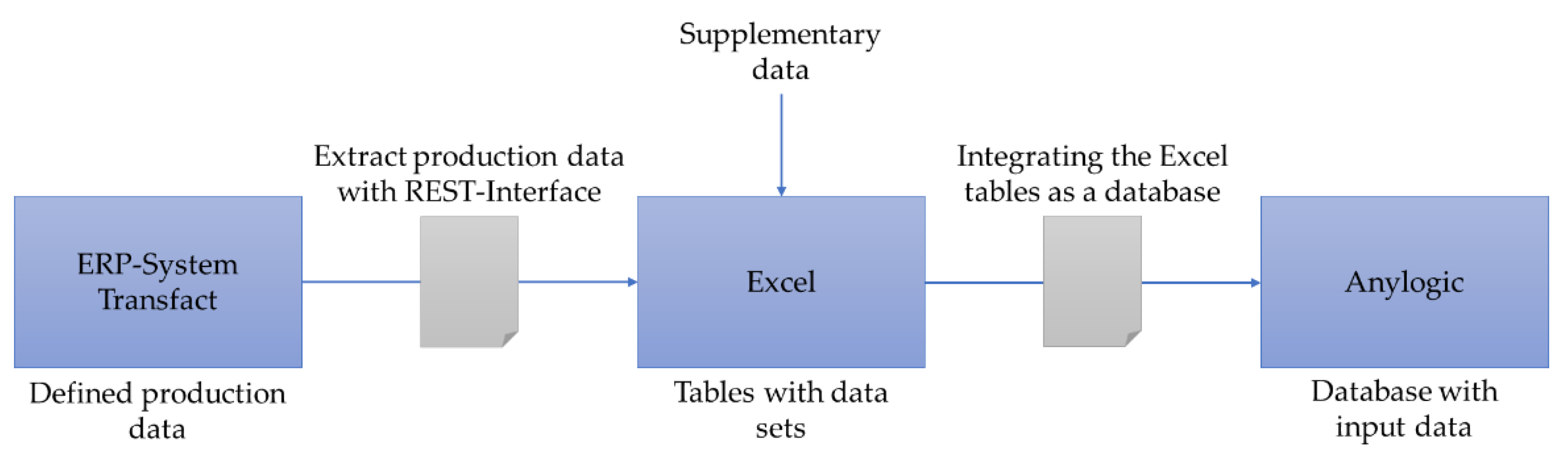
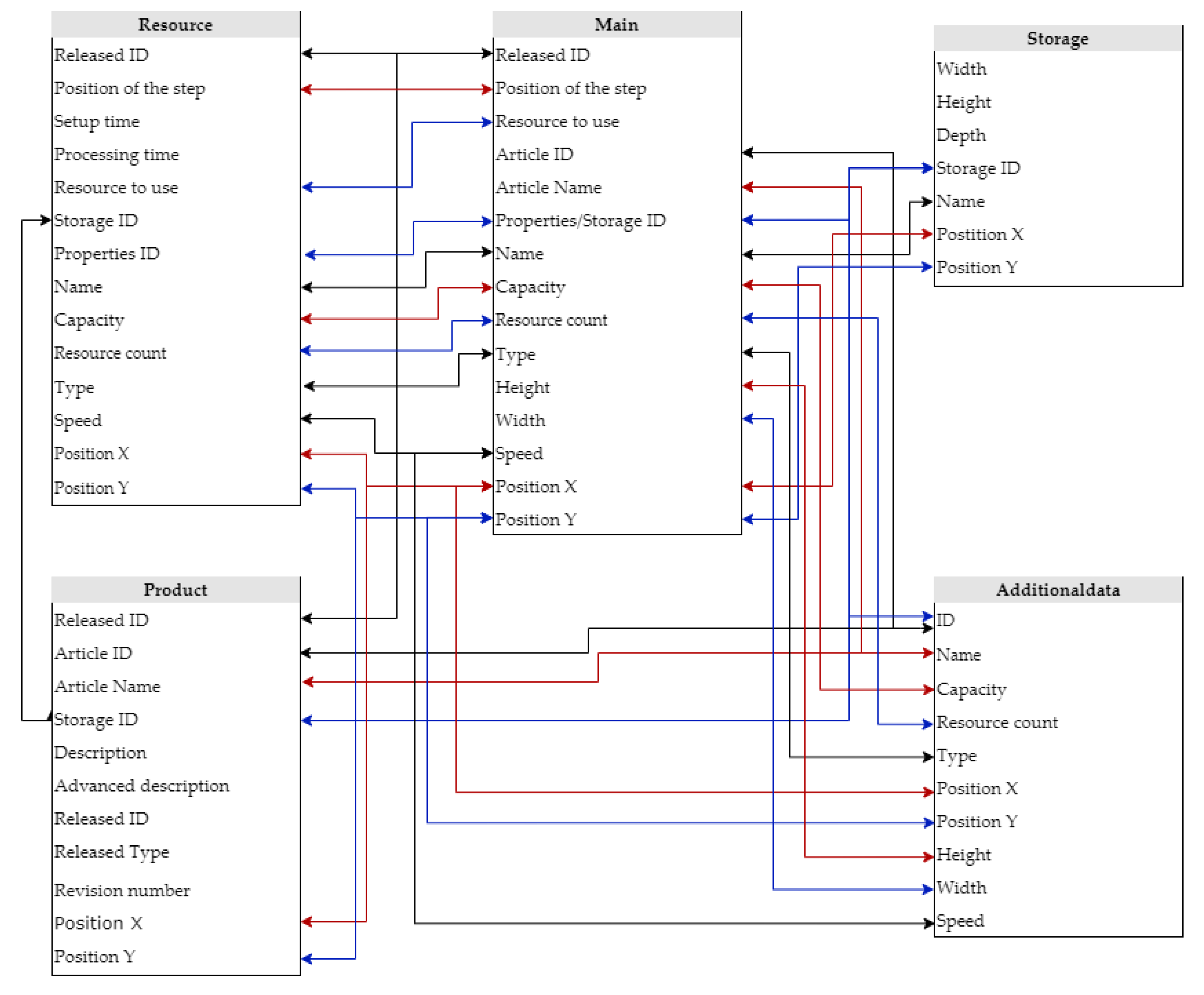
3.1. Description of the Data Transfer

The data of the learning factories are stored in the ERP system TransfactTM, which contains data on the articles, their work cards with the routing steps, the warehouses, and the resources used. In general, the Transfact™ ERP system is a completely web-based system for companies in production, trade, and services. It offers the choice of several modules that can be selected and configured according to specific needs. According to the ERP provider, Transfact™ stands for a transparent factory, in which one can view real-time information on current production, sales, inventory, and purchasing status at any time [58]. TransfactTM uses a SQL database [59,60]. For simulation purposes, the database is accessed by a REST interface, which allows easy downloading of the desired data tables with the aid of filters. After downloading, the tables are transferred to the model folder of the generic simulation.
The model folder also contains the Excel spreadsheet with supplementary data for the agent’s transport route, which is not contained in the ERP system. The ERP data and the supplementary data are prepared for simulation usage via a macro. The entire data transfer between Transfact™ and AnyLogic™ is presented in Figure 2.

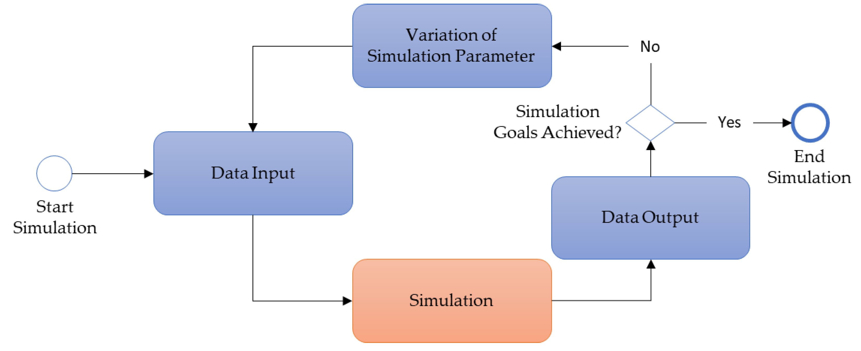
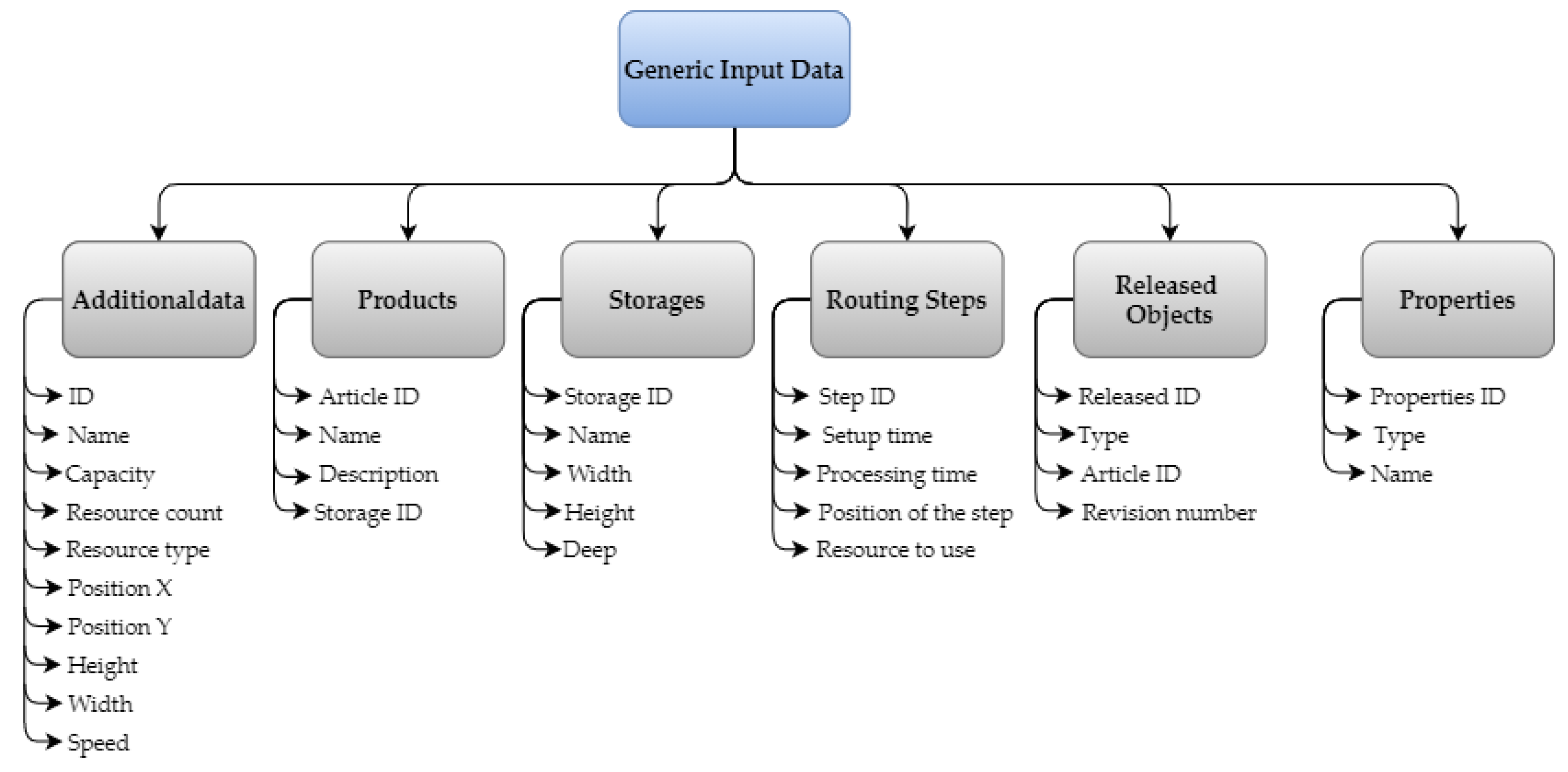
3.2. Generic Structure of the Simulation

The generic simulation is based on a multi-method model. It uses two modelling methods that complement each other: agent-based modelling (ABM) and discrete-event modelling (DEM). DEM is responsible for routing agents in the simulation. It handles the work steps and decides, for example, which resource has to be approached next, and it is also used for statistical evaluations. With ABM, processes such as the parameterisation of resources (e.g., transporters, workstations) are done. ABM has an advantage in that all essential parameters can be found bundled in the respective agent. Likewise, the representations of resources, warehouses, and products are defined via the respective agents of ABM. The generic AnyLogicTM simulation model requires six input data sets to build and parameterise the model. These data are to be extracted from the ERP system TransfactTM. A variety of information is available within these data sets, some of them required for the generic simulation model. All necessary production parameters can be seen in Figure 3. These include the respective IDs of the data records for unique identification and assignment, such as the article ID. The names of the data sets are specified by TransfactTM and are processed accordingly in the generic model.
The digital twin model in the generic AnyLogicTM simulation consists of the main agent and three agent populations (see Figure 4). There is one agent population each for the product, warehouse, and resource. These named agent populations live in the generic simulation environment and are defined by the ‘Main’ agent, which is responsible for the organisation of the simulation. It links the individual populations with one another and with the simulation and takes over both the visualisation of the digital twin model as well as the evaluations and presentations of the statistics. The individual behaviour of the agents is defined by the assigned parameters, the contained functions, and DEM elements from AnyLogicTM. An agent population can contain multiple agents in two ways. The number of populations is defined by the ERP system TransfactTM and the user. On the one hand, an agent population can represent different agents, such as products A and B, moving resource A (e.g., forklift), and static resource A (e.g., machining centre). In this case, each agent has to be considered separately with its parameters and specifications. On the other hand, an agent with the same parameters can appear multiple times in the simulation model. Simplified, this means that an agent is copied. The number of these copies or the number of resources is taken from the agent additions (see Figure 3).
Each entry in the records has a unique ID number, which enables the linking of data in the generic simulation (see Figure 4). The ‘Main’ agent and the three agent populations ‘Resource’, ‘Storage’, and ‘Product’ are linked to one another via their parameters. Only the most important parameters are shown in the figure. Parameters with relationships with other agents are listed only. For completeness, the supplementary data or ‘additional data’ parameters are also listed, even if this is not an agent but a data table because the agent populations also get their parameters from an associated data table. In addition, the individual agents require specific parameters from the ‘additional data’ that are important for the visualisation of the digital twin model. The ‘Main’ agent is located in the centre, demonstrating that it forms the organisational structure and is responsible for connecting the individual parameters and agent populations.

3.3. Generic Visualisation

The generic simulation automatically creates a suitable visualisation of the considered production system via a two-dimensional representation. The user can choose between two types of visualisation: pre-defined representations by AnyLogic™ and individual representations of the resources, warehouses, and products. Figure 5 shows the visualisation of Workstation 1 of Learning Factory 4.0 as a digital presentation (b) with a correspondingly selected symbol. Moreover, the user can select an individual production layout as the background for the visualisation. The layout has to be individually integrated into the simulation by the user. However, the selection of images and layouts is not mandatory for the simulation to run. In this case, predefined symbols are displayed by default in the visualisation.

3.4. Generic Statistical Evaluation Using Defined Key Performance Indicators

The generic simulation uses KPIs to evaluate the considered production system. For this approach, the generic simulation provides predefined KPIs in a configurable display. The user can choose among numerous statistical evaluations, which can be selected in any combination. For specific KPIs, one can also choose among different diagram types for display. For example, when displaying the individual utilisation of resources, only a bar chart is available. On the other hand, the users can choose among a bar chart, a pie chart, or a plot for the KPIs in the presentation of produced articles. Figure 6 shows an overview of the available diagram types. In (a), the number of items produced is shown in a plot, while (b) shows the utilisation of all resources in a bar chart. Finally, the waiting times of the respective resources are represented in a pie chart in (c). For KPIs, multiple chart types are useful, and the desired chart type can be selected via radio buttons.
In the simulation, different variables are measured within the agents, and these variables are used to calculate the KPIs. The used KPIs are listed in Table 2 with corresponding definitions:
In summary, the user of the generic simulation has various options for displaying the production as a digital twin and numerous KPI evaluations. Thus, one can simulate the digital twin generically with a high recognition value. However, the list of considered KPIs can be extended or reduced depending on the considered optimisation problem and requirements of the production system owner.

4. Proof of Concept

A case study was conducted to verify the concept of the generic simulation model. In this case study, a learning factory was used to demonstrate how a digital twin was generically generated from this. Finally, the discussion clarifies the differences to other publications and places the results in the state of the art of the research.

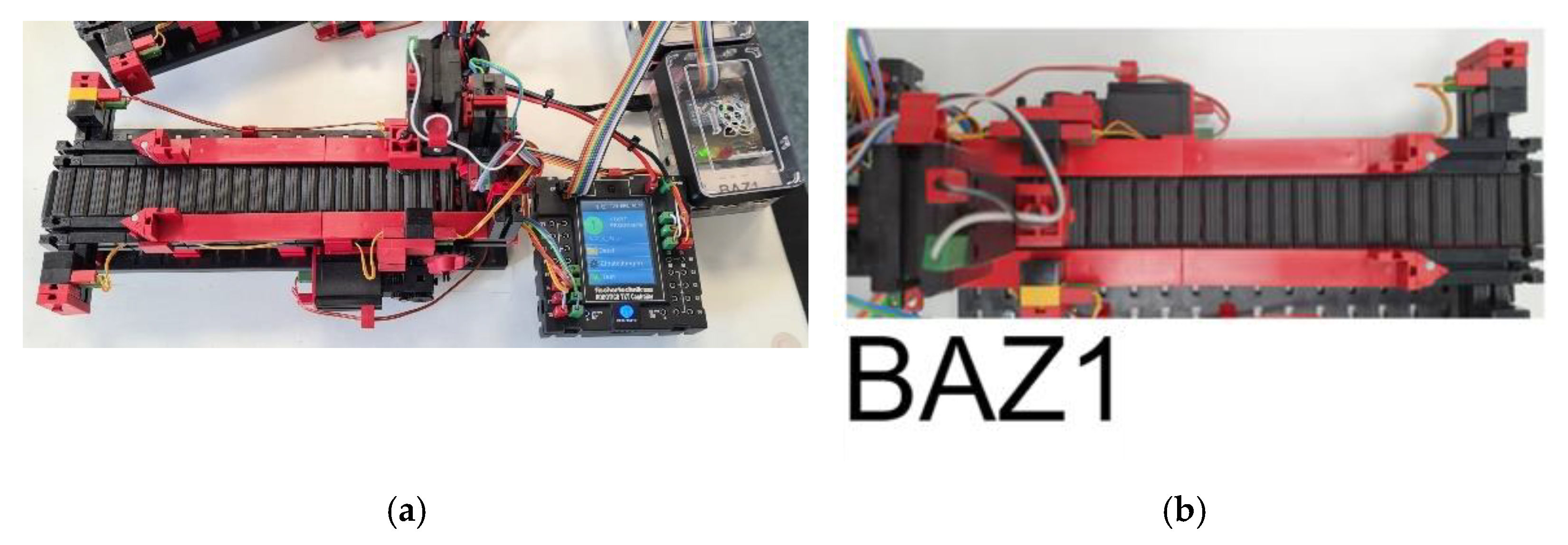
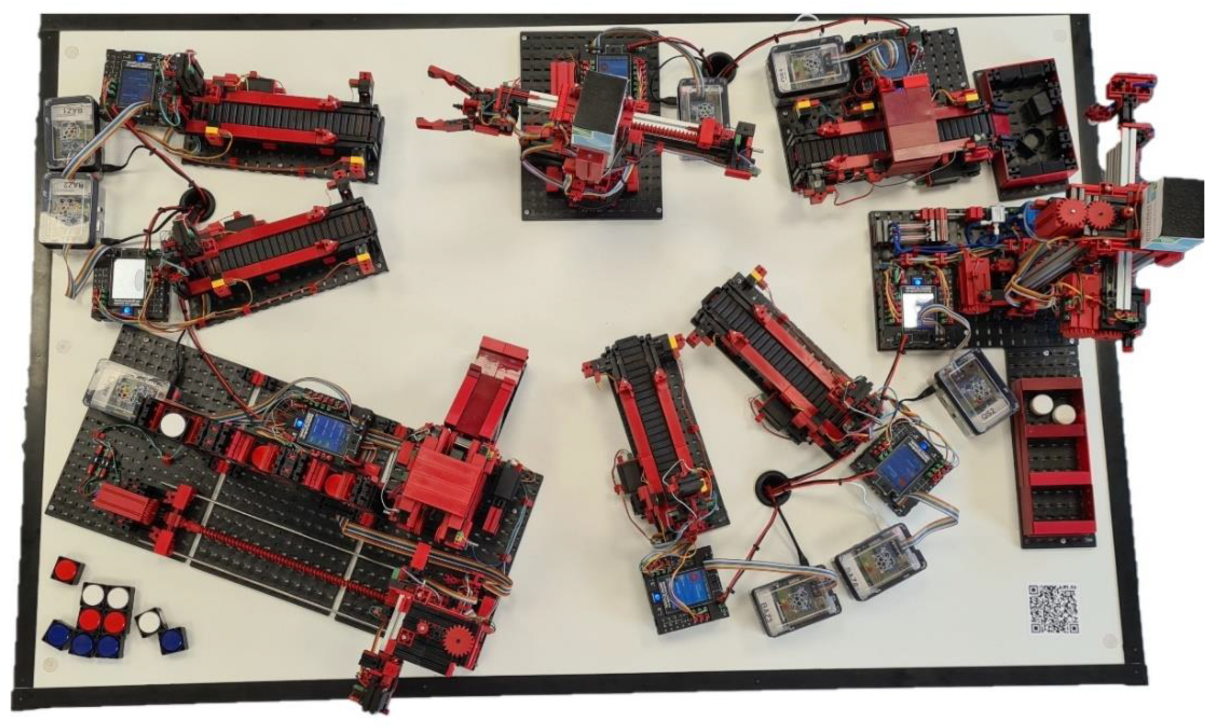
4.1. Scope of the Case Study

The case study aims to verify the concept of the generic simulation model in AnyLogicTM as well as to check the functions evaluating and visualising the physical system. For this approach, a learning factory—the Fischertechnik production system (FTPS)—is considered to prove the concept.
The FTPS has been realised through student projects at the University of Applied Sciences Emden/Leer [62]. It consists of modules from the Fischertechnik construction kit (see Figure 7). The individual modules are connected to a Raspberry Pi via the Fischertechnik PLC (the TXT controller). The individual modules of the system (workstations, transport robots, warehouse) are implemented as a job shop production system. The resources act autonomously and independently of one another. The FTPS is a laboratory setup with an incoming warehouse, an outgoing warehouse, four machining centres, a quality inspection centre, and three robots for material handling (see Figure 7). Three different products (white, red, and blue cylinders) are produced in the production system. These are processed in a predefined product mix. Each of the products uses two of the four machining centres, with no product sequence being the same [62].
Two validation options were considered for testing the generic simulation on the existing FTPS. The first is a comparison of the generic process with the physically existing production system. The comparison of produced quantities is unfavourable for a continuous test because, in the physical system, the receiving warehouse has a defined stock of three products each. This means that it has to be restocked manually again and again. In the generic simulation, this is done automatically after an inter-arrival time has elapsed. Second, in the real model, there is a possibility that cylinders would be stuck at random times. Such cases are not simulated. A non-generic and specific simulation was used to compare the number of pieces produced per time. With this specific simulation, a comparison could be made with the generic simulation.

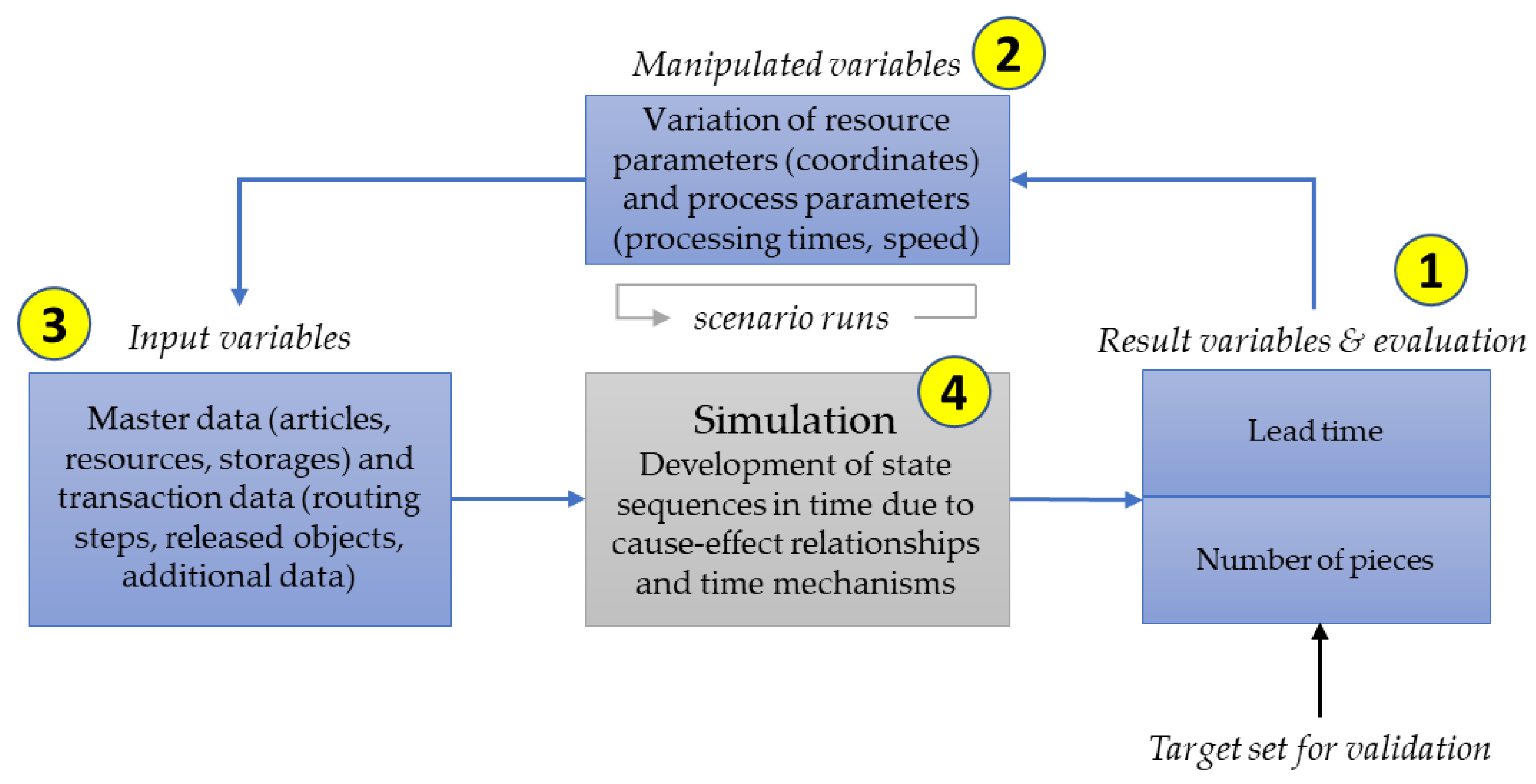
4.2. Procedure for Validation of the Case Study

Figure 8 describes the evaluation of the digital twin of the generic simulation using physical model data. The following variables are selected to compare the generic simulation with the physical learning factory:
  • Lead time
  • Number of units produced per article type
The time per work step is reported back to Transfact™ by the physical FTPS and is stored in the corresponding completion batch. From this, the lead time can be calculated. The feedback in Transfact™ is done in minutes. The resulting lead time is accordingly also only accurate to the minute and is additionally measured in the physical system using a stopwatch. It is measured as the time between picking up an item from the robot in the incoming warehouse and the end of the robot’s retrieval in the outgoing warehouse. The lead time in the simulation is measured in the main agent, between the source for creating the item and the sink for completing the item. In the comparison between the generically simulated and the physical Fischertechnik production plants, the basic processes were compared for correctness. The lead times for four different processes were compared:
  • Production of a blue cylinder (3 runs)
  • Production of a white cylinder (3 runs)
  • Production of a red cylinder (3 runs)
  • Production of a sequence of blue, red, and white cylinders (1 run)
Three runs were carried out in the physical system for the individual types of cylinders as the lead times vary here. The variation results from unexpected maintenance, reefing of the robot, or other disturbances in the physical system. For the generic simulation, no disturbances are simulated, which is why all three runs result in the same lead time. For the production sequence, a run with the order blue, red, and white was performed for both the physical system and the generic simulation.
Another comparative value is the number of units produced per article type–the production efficiency. This is measured in the simulation at the end of the process chain by counting up the associated variable per manufactured article. A simulation time of 105 h was selected to obtain meaningful values and identify any differences in the number of units produced. This time results from the time for a production week, i.e., three shifts with seven hours each on five working days.

4.3. Results and Discussion of the Case Study

In the following section, the validation results are presented. The simulation is tested for logic and production times, and the implemented automatic algorithms are verified. Moreover, the KPIs and resource visualisations are tested. Finally, a discussion is provided to place the generic simulation from this paper in a broad context.

4.3.1. Test of Statistical Functions

First of all, the processing of each work step should be checked. For this purpose, only one product was controlled at a time. This was done individually for each product. The aim was to check whether the respective work steps were processed and used correctly in the generic simulation. The respective lead times for a part should be close to one another or identical. For the ERP system and the physical system, the time range was shown for three runs. The scatter can be explained by the fact that the robot starting positions were different and that the transport robot returns to its reference position from time to time. The spread in the ERP system is 60 seconds because the time in Transfact™ is given in minutes only. The lead times for the production of one cylinder at a time in the simulation were always within the scatter of the ERP system and the physical system (see Table 3). One could see that for the FTPS, the processing sequence with the times was close to the physical system. Since unscheduled maintenance can occur in the physical production system, a fourth test was performed to show the difference in lead times for three products in a row. In addition, the interaction of the overall system was to be checked. Apart from minor differences in maintenance times, the lead times were close to one another when running a production mix (see Table 3). The travel distance of the robots and the processing sequence were also similar. The gap in the ERP system arises from the fact that the time is only specified to the minute.
Next, the production output is checked. After 105 hours, 763 blue, red, and white cylinders were produced (see Figure 9) in both (a) the non-generic simulation and (b) the generic simulation. This result indicates that the production works evenly and that the generic simulation gives the same results as the non-generic simulation.

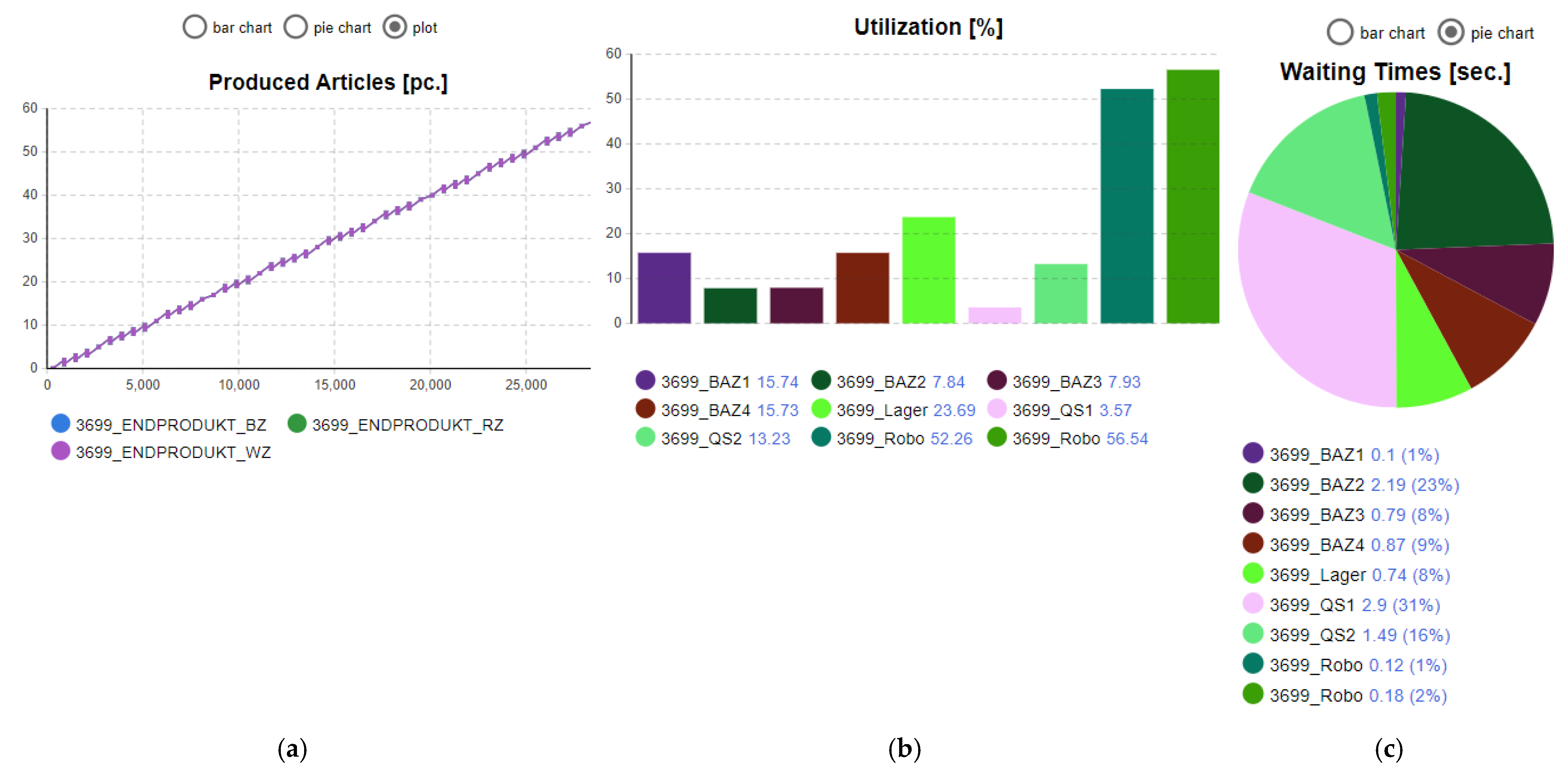
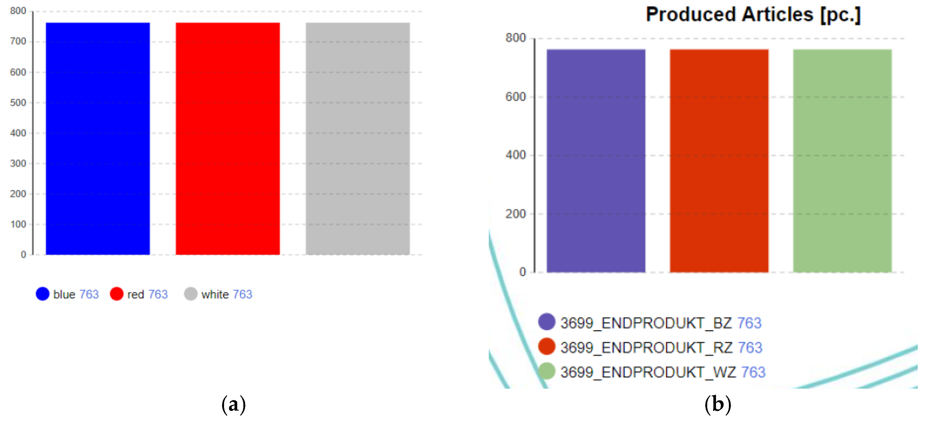
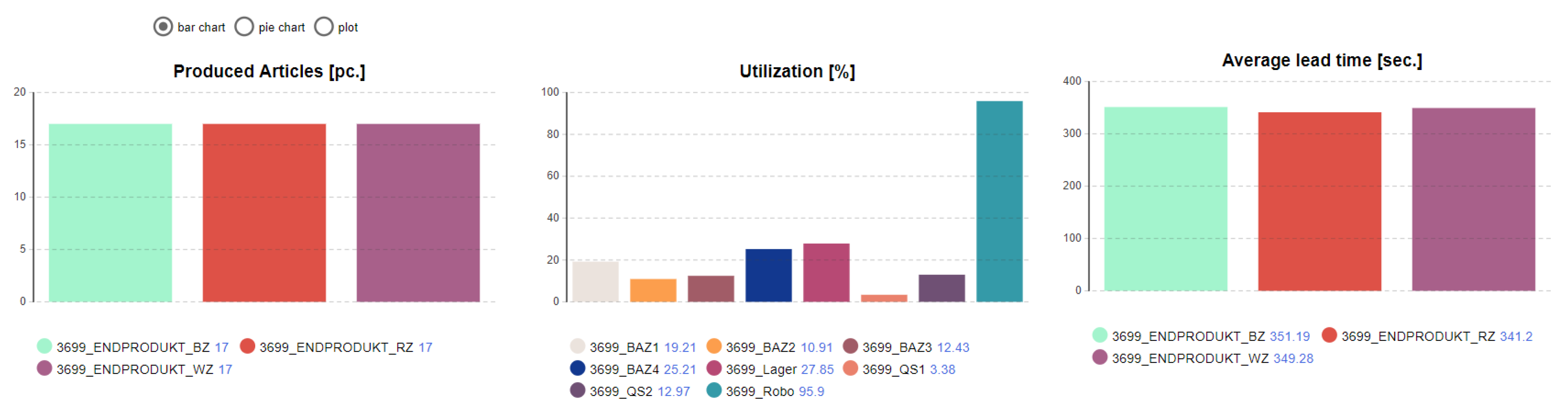
4.3.2. Visualisation Results

Bar charts were predominantly used for the statistical analysis, but other charts can be applied as well. Figure 10 shows an example of the FTPS as well as the produced articles, the utilisation, and the average lead time. The displayable KPIs are as follows:
  • Produced articles
  • Produced articles per time
  • Utilisation
  • Work in progress
  • Waiting times
  • Takt time
  • Lead time (last article)
  • Average lead time
  • Process time
  • Queues
The representation allows a direct comparison of the KPIs. In this way, the articles are produced evenly in the FTPS, and the lead times per article are also close together. Additionally, the bottleneck of the production can be recognised directly with the extent of utilisation. The robot for the material transport between the processing centres can be identified as a bottleneck because this has much higher utilisation than all other resources. With this evaluation, production optimisation can be facilitated, and production planning can thus be strongly supported.

4.3.3. Discussion

The generic simulation can independently create a simulation based on defined input data and perform a statistical evaluation with the help of these data. The time required for the creation depends on the initial data situation. If the data in the ERP system are complete, the simulation can be created within a few hours. For the FTPS, a specific non-generic simulation was created in addition to the generic simulation. The time required to create the specific simulation differs depending on the level of detail. However, at least one week is needed for the creation. Accordingly, the creation of a digital twin with a generic simulation brings significant time advantages even for simple production, such as the FTPS.
Another point of the simulation presented in this paper is the use of the simulation program AnyLogicTM. Since AnyLogicTM supports multi-method modelling, ABM can be used in addition to the discrete-event model. The input data of the simulation are stored in different agents, which communicate with one another in the simulation only using the routing steps. The basic organisation is performed via DEM logic. All other publications found use only DEM for the generic simulation, which is limited in its abstractness. These limit, for example, the inherent dynamics of the items to be produced. Other publications reach their limits the more complex and dynamic the system gets. Because of ABM, modelling, even to the highest level of abstraction, is possible. This level of abstraction makes it possible to simulate not only flow production but also job shop production. Flow production is the most common form of production simulated in the other publications.
A further difference from the other generic simulations found in the literature is the procurement of the input data. Because of the REST interface, a connection to the ERP system TransfactTM or any other ERP system is possible. Only the publication by Mertins et al. [48] also uses an ERP system to generate the input data for the generic simulation. Here, the intermediate storage takes place in Access. However, the simulation based on this also uses DEM with the simulation program ARENA™ [63]. Therefore, the input data are stored in arrays. This is a restriction of variability. Furthermore, this generic simulation primarily enables factory planning. In contrast, the presented generic simulation model offers visualisation and optimisation of the existing production or the production to be designed.

5. Conclusions and Outlook

In this paper, a generic simulation was presented. The generic simulation uses ERP data sets as the main input data. Based on these input data, the generic simulation can create a digital twin of real production. The developed digital twin helps production planning to optimise future production programs. Moreover, the digital twin enables small- and medium-sized companies to design their production more efficiently and in a more targeted manner without costly test setups. The results showed that the generic simulation is capable of correctly representing the learning factory in a lab environment.
However, the presented concept and case study offers several limitations and future works. The case study is limited to a learning factory in a lab environment. The lab environment provides ideal conditions simulating the learning factory in order to collect required input datasets and analysing output data. Moreover, the simulation developer can easily understand and verify the simplified production processes of the learning factory to create the digital twin. The simulation of industrial production processes is more challenging than the learning factory because of, e.g., incomplete input data or lack of output data to verify the simulation results. Moreover, additional support is required to compare the digital twin with the real production system. Therefore, it is recommended that the simulation developers work together with the production managers to create the digital twin as correctly as possible.
For this approach, the visualisation of the production needs to be improved further to increase the identification of the digital twin, e.g., by adding real transport routes of the production. This way, the transporters and products can also use existing transport routes. In addition, the generic simulation produces products without a time limit. Therefore, the implementation of a shift schedule is recommended. The learning factory products are produced in a lot size of one. It would be interesting to produce articles with a lot size greater than one.
Another limitation is that resource failures or breakdowns are not considered in the simulation model. For this approach, the simulation model and input datasets need to be extended by variables and parameters to represent the probability of machine failures and breakdowns and the opportunity for machine maintenance to avoid breakdowns. Moreover, the result visualizations need to be adapted to represent the distribution of, e.g., lead time, delivery dates, and machine utilization.

Author Contributions

A.P. contributed the general idea and concept; S.K. and H.T. conceived, designed and performed the experiments; S.K. and H.T. analyzed the data; M.Z. and A.P. contributed materialsand ideas; S.K., H.T., M.Z. and A.P. wrote, reviewed and edited the paper. All authors have read and agreed to the published version of the manuscript.

Funding

This research received no external funding.

Institutional Review Board Statement

Not applicable.

Informed Consent Statement

Not applicable.

Data Availability Statement

No data availability statements.

Conflicts of Interest

The authors declare no conflict of interest.

References

  1. März, L.; Krug, W.; Rose, O.; Weigert, G. Simulation und Optimierung in Produktion und Logistik: Praxisorientierter Leitfaden mit Fallbeispielen; Springer: Berlin/Heidelberg, 2011; ISBN 9783642145360. [Google Scholar]
  2. Million, C. Crashkurs Blockchain-inkl. Arbeitshilfen Online, 1st ed.; Haufe, L., Ed.; C.H. Beck eLibrary: Freiburg, München, 2019; ISBN 978-3-648-12347-8. [Google Scholar]
  3. MAIT. MAIT. Available online: https://www.mait.de/trends-und-innovationen-studie-simulation (accessed on 12 May 2021).
  4. Overbeck, L.; Brützel, O.; Stricker, N.; Lanza, G. Digitaler Zwilling des Produktionssystems. Zeitschrift für wirtschaftlichen Fabrikbetrieb 2020, 115, 62–65. [Google Scholar] [CrossRef]
  5. SimPlan, A.G. SimPlan AG | Der führende Simulationsdienstleister in DACH. Available online: https://www.simplan.de/ (accessed on 17 May 2021).
  6. SimPlan, A.G. Simulation in der Produktion|Planung und Optimierung. Available online: https://www.simplan.de/services/produktion/ (accessed on 17 May 2021).
  7. SimPlan, A.G. Unsere Referenzen-Zufriedene Kunden sprechen für unsere Qualität|. Available online: https://www.simplan.de/referenzen/ (accessed on 20 April 2021).
  8. Statista. Audi AG-Mitarbeiterzahl 2020|Statista. Available online: https://de.statista.com/statistik/daten/studie/36001/umfrage/mitarbeiterzahl-des-automobilherstellers-audi/ (accessed on 5 May 2021).
  9. Statista. ZF Friedrichshafen AG-Mitarbeiter|Statista. Available online: https://de.statista.com/statistik/daten/studie/159950/umfrage/anzahl-der-mitarbeiter-der-zf-friedrichshafen-ag/ (accessed on 5 May 2021).
  10. Statista. Trumpf Gruppe-Anzahl der Mitarbeiter bis 2020|Statista. Available online: https://de.statista.com/statistik/daten/studie/222174/umfrage/anzahl-der-mitarbeiter-der-trumpf-gruppe/ (accessed on 7 June 2021).
  11. TRUMPF GmbH + Co. KG. Available online: https://www.trumpf.com/de_DE/ (accessed on 7 June 2021).
  12. Wenzel, S.; Peter, T. Simulation in Produktion und Logistik 2017; Kassel University Press: Kassel, Germany, 2017; ISBN 9783737601931. [Google Scholar]
  13. Zarte, M.; Wunder, U.; Pechmann, A. Concept and first case study for a generic predictive maintenance simulation in AnyLogicTM. In Proceedings of the IECON 2017-43nd Annual Conference of the IEEE Industrial Electronics Society: China National Convention Center, Bejing, China, 29 October–1 November 2017; IEEE: Piscataway, NJ, USA, 2017; pp. 3372–3377, ISBN 9781538611272. [Google Scholar]
  14. Zarte, M.; Wunder, U.; Pechmann, A. Concept and Demonstration of a Generic Simulation to Identify Production Bottlenecks. In Proceedings of the IEEE 16th International Conference on Industrial Informatics (INDIN): Faculty of Engineering of the University of Porto, Porto, Portugal, 18–20 July 2018; IEEE: Piscataway, NJ, USA, 2018; pp. 849–854, ISBN 9781538648292. [Google Scholar]
  15. Duden. Generisch. Available online: https://www.duden.de/rechtschreibung/generisch (accessed on 5 May 2021).
  16. Transfact GmbH Industrial Engineering & Software Solutions. Available online: https://www.transfact.de/ (accessed on 21 June 2021).
  17. Mackulak, G.T.; Lawrence, F.P.; Colvin, T. Effective simulation model reuse: A case study for AMHS modeling. In Proceedings of the Simulation Conference Proceedings, Washington, DC, USA, 13–16 December 1998; IEEE: Piscataway, NJ, USA, 1998; pp. 979–984, ISBN 0-7803-5133-9. [Google Scholar]
  18. VDI Society Production and Logistics. Simulation of Systems in Materials Handling, Logistics and Production-Fundamentals, 2014-12-00 (VDI 3633 Part 1), VDI-Gesellschaft Produktion und Logistik (GPL).
  19. Gutenschwager, K.; Rabe, M.; Spieckermann, S.; Wenzel, S. Simulation in Produktion und Logistik: Grundlagen und Anwendungen; Springer Vieweg: Berlin, Germany, 2017; ISBN 3662557444. [Google Scholar]
  20. Stefan, B.; Christoph, H.; Roland, R. Next Generation Digital Twin. In Proceedings of the TMCE 2018, Las Palmas de Gran Canaria, Spain, 7 May 2018. [Google Scholar]
  21. Tao, F.; Zhang, H.; Liu, A.; Nee, A.Y.C. Digital Twin in Industry: State-of-the-Art. IEEE Trans. Ind. Inf. 2019, 15, 2405–2415. [Google Scholar] [CrossRef]
  22. Fraunhofer-Gesellschaft. Digitalization Is Changing the Future of Manufacturing. Available online: https://www.fraunhofer.de/en/research/current-research/production-4-0.html (accessed on 7 June 2021).
  23. Ilya, G. Anylogic in Three Days: A Quick Course in Simulation Modeling, 5th ed. Available online: https://www.anylogic.com/upload/al-in-3-days/anylogic-in-3-days.pdf (accessed on 7 June 2021).
  24. Hallgren, M.; Olhager, J.; Schroeder, R.G. A hybrid model of competitive capabilities. Int. J. Oper. Prod. Mnagemnt 2011, 31, 511–526. [Google Scholar] [CrossRef]
  25. Schroer, B.J.; Farrington, P.A.; Swain, J.J.; Utley, D.R. A generic simulator for modeling manufacturing modules. In Proceedings of the 28th Conference on Winter Simulation, Coronado, CA, USA, 8 November 1996; IEEE: Piscataway, NJ, USA, 1996; pp. 1155–1160, ISBN 0-7803-3383-7. [Google Scholar] [CrossRef] [Green Version]
  26. Negahban, A.; Smith, J.S. Simulation for manufacturing system design and operation: Literature review and analysis. J. Manuf. Syst. 2014, 33, 241–261. [Google Scholar] [CrossRef]
  27. Mourtzis, D.; Doukas, M.; Bernidaki, D. Simulation in Manufacturing: Review and Challenges. Procedia CIRP 2014, 25, 213–229. [Google Scholar] [CrossRef] [Green Version]
  28. Steinhausen, D. Simulationstechniken; Walter de Gruyter GmbH: München, Germany, 2019; ISBN 9783486785043. [Google Scholar]
  29. White, K.P.; Ingalls, R.G. The Basics of Simulation. In Proceedings of the 2018 Winter Simulation Conference, Gothenburg, Sweden, 9–12 December 2018; ISBN 9781538665725. [Google Scholar]
  30. Andrei Borshchev, A.F. From system dynamics and discrete event to practical agent based modeling: Reasons, techniques, tools. In Proceedings of the 22nd International Conference of the System Dynamics Society, Oxford, UK, 25–29 July 2004. [Google Scholar]
  31. Nguyen, A.-T.; Reiter, S.; Rigo, P. A review on simulation-based optimization methods applied to building performance analysis. Appl. Energy 2014, 113, 1043–1058. [Google Scholar] [CrossRef]
  32. Uhlig, T.; Rose, O. Simulation-based optimization for groups of cluster tools in semiconductor manufacturing using simulated annealing. In Proceedings of the 2011 Winter Simulation Conference—(WSC 2011), Phoenix, AZ, USA, 11 December 2011; Staff, I., Ed.; pp. 1852–1863, ISBN 978-1-4577-2109-0. [Google Scholar]
  33. Wincheringer, W.; Sekulic, M.; Kexel, M. Generisches Simulationsmodell für automatische Hochregallagersysteme. In Proceedings of the ASIM SST 2020, Sankt Augustin, Germany, 14–15 October 2020; Deatcu, C., Lückerath, D., Ullrich, O., Durak, U., Eds.; ARGESIM: Wien, Austria, 2020; pp. 389–395, ISBN 978-3-901608-93-3. [Google Scholar] [CrossRef]
  34. Lienert, T.; Fottner, J. Entwicklung einer generischen Simulationsmethode für das zeitfensterbasierte Routing Fahrerloser Transportfahrzeuge. Logist. J. Proc. 2017, 10. [Google Scholar] [CrossRef]
  35. Meng, C.; Nageshwaraniyer, S.S.; Maghsoudi, A.; Son, Y.-J.; Dessureault, S. Data-driven modeling and simulation framework for material handling systems in coal mines. Comput. Ind. Eng. 2013, 64, 766–779. [Google Scholar] [CrossRef]
  36. Jones, D.; Snider, C.; Nassehi, A.; Yon, J.; Hicks, B. Characterising the Digital Twin: A systematic literature review. CIRP J. Manuf. Sci. Technol. 2020, 29, 36–52. [Google Scholar] [CrossRef]
  37. Negri, E.; Fumagalli, L.; Macchi, M. A Review of the Roles of Digital Twin in CPS-based Production Systems. Procedia Manuf. 2017, 11, 939–948. [Google Scholar] [CrossRef]
  38. Stark, R.; Damerau, T. Digital Twin. CIRP Encycl. Prod. Eng. 2019, 66, 1–8. [Google Scholar] [CrossRef]
  39. Kritzinger, W.; Karner, M.; Traar, G.; Henjes, J.; Sihn, W. Digital Twin in manufacturing: A categorical literature review and classification. IFAC-Pap. 2018, 51, 1016–1022. [Google Scholar] [CrossRef]
  40. Zheng, Y.; Yang, S.; Cheng, H. An application framework of digital twin and its case study. J. Ambient. Intell. Hum. Comput. 2019, 10, 1141–1153. [Google Scholar] [CrossRef]
  41. Guo, J.; Zhao, N.; Sun, L.; Zhang, S. Modular based flexible digital twin for factory design. J. Ambient. Intell. Hum. Comput. 2019, 10, 1189–1200. [Google Scholar] [CrossRef]
  42. Goodall, P.; Sharpe, R.; West, A. A data-driven simulation to support remanufacturing operations. Comput. Ind. 2019, 105, 48–60. [Google Scholar] [CrossRef]
  43. Pidd, M. Guidelines for the design of data driven generic simulators for specific domains. Simulation 1992, 59, 237–243. [Google Scholar] [CrossRef]
  44. Brown, N.A. Model flexibility: Development of a generic data-driven simulation. In Proceedings of the 2010 Winter Simulation Conference (WSC 2010), Baltimore, MD, USA, 5–8 December 2010; [incorporating the MASM (Modeling and Analysis for Semiconductor Manufacturing) Conference]. Johansson, B., Ed.; IEEE: Piscataway, NJ, USA, 2010; pp. 1366–1375, ISBN 978-1-4244-9865-9. [Google Scholar]
  45. Schroeder, G.N.; Steinmetz, C.; Pereira, C.E.; Espindola, D.B. Digital Twin Data Modeling with AutomationML and a Communication Methodology for Data Exchange. IFAC-Pap. 2016, 49, 12–17. [Google Scholar] [CrossRef]
  46. Samaranayake, P. Enhanced Data Models for Master and Transaction Data in ERP Systems-Unitary Structuring Approach. In Proceedings of the International Multi Conference of Engineers and Computer Scientists 2008 (IMECS 2008), Hong Kong, China, 19–21 March 2008; Volume II, pp. 19–21. [Google Scholar]
  47. Wang, J.; Chang, Q.; Xiao, G.; Wang, N.; Li, S. Data driven production modeling and simulation of complex automobile general assembly plant. Comput. Ind. 2011, 62, 765–775. [Google Scholar] [CrossRef]
  48. Mertins, K.; Rabe, M.; Gocev, P. Integration of Factory Planning and ERP/MES Systems: Adaptive Simulation Models. In Lean Business Systems and Beyond; Koch, T., Ed.; International Federation for Information Processing: Boston, MA, USA, 2008; pp. 185–193. ISBN 978-0-387-77248-6. [Google Scholar] [CrossRef] [Green Version]
  49. Chapman, S.N. The Fundamentals of Production Planning and Control; Pearson/Prentice Hall: Upper Saddle River, NJ, USA, 2006; ISBN 978-0130176158. [Google Scholar]
  50. Hübl, A.; Altendorfer, K.; Jodlbauer, H.; Gansterer, M.; Hartl, R.F. Flexible model for analyzing production systems with discrete event simulation. In Proceedings of the 2011 Winter Simulation Conference, Phoenix, AZ, USA, 11–14 December 2011; Jain, S., Ed.; IEEE: Piscataway, NJ, USA, 2011; pp. 1554–1565, ISBN 9781457721083. [Google Scholar] [CrossRef] [Green Version]
  51. Altendorfer, K.; Felberbauer, T.; Gruber, D.; Hübl, A. Application of a generic simulation model to optimize production and workforce planning at an automotive supplier. In Proceedings of the Winter Simulation Conference (WSC), JW Marriott, Washington, DC, USA, 8–11 December 2013; [Including the 9th International Conference on Modeling and Analysis of Semiconductor Manufacturing (MASM 2013)]. Pasupathy, R., Ed.; IEEE: Piscataway, NJ, USA, 2013; pp. 2689–2697, ISBN 978-1-4799-3950-3. [Google Scholar]
  52. Felberbauer, T.; Altendorfer, K.; Hubl, A. Using a scalable simulation model to evaluate the performance of production system segmentation in a combined MRP and kanban system. In Proceedings of the 2012 Winter Simulation Conference, Berlin, Germany, 9–12 December 2012; Staff, I., Ed.; pp. 1–12, ISBN 978-1-4673-4782-2. [Google Scholar]
  53. Lim, D.-E.; Seo, M. A Generic Simulation Framework for Efficient Simulation Analyses for Semiconductor Manufacturing: A Case Study. IJCA 2014, 7, 75–84. [Google Scholar] [CrossRef] [Green Version]
  54. Lee, J.Y.; Kang, H.S.; Kim, G.Y.; Noh, S.D. Concurrent material flow analysis by P3R-driven modeling and simulation in PLM. Comput. Ind. 2012, 63, 513–527. [Google Scholar] [CrossRef]
  55. Akiya, N.; Bury, S.; Wassick, J.M. Generic framework for simulating networks using rule-based queue and Resource-Task Network. In Proceedings of the 2011 Winter Simulation Conference, Phoenix, USA, 11–14 December 2011; Jain, S., Ed.; IEEE: Piscataway, NJ, USA, 2011; pp. 2189–2200, ISBN 9781457721083. [Google Scholar]
  56. Wy, J.; Jeong, S.; Kim, B.-I.; Park, J.; Shin, J.; Yoon, H.; Lee, S. A data-driven generic simulation model for logistics-embedded assembly manufacturing lines. Comput. Ind. Eng. 2011, 60, 138–147. [Google Scholar] [CrossRef]
  57. Kibira, D.; McLean, C.R. Generic simulation of automotive assembly for interoperability testing. In Proceedings of the 2007 Winter Simulation Conference, Washington, DC, USA, 9–12 December 2007; IEEE Service Center: Piscataway, NJ, USA, 2007; pp. 1035–1043, ISBN 978-1-4244-1305-8. [Google Scholar]
  58. Transfact GmbH. Startseite. Available online: https://www.transfact.de/ (accessed on 18 May 2021).
  59. Aragon, M. Add-Ons. Available online: https://www.transfact.de/features/add-ons/ (accessed on 5 May 2021).
  60. Kostenoptimierte und Leistungsstarke Datenbank. Available online: https://www.oracle.com/de/database/ (accessed on 5 May 2021).
  61. APICS Dictionary, 13th ed.; Blackstone, J.H. (Ed.) APICS: Alexandria, VA, USA, 2010; ISBN 978-0-615-39441-1. [Google Scholar]
  62. Zarte, M.; Wermann, J.; Heeren, P.; Pechmann, A. Concept, Challenges, and Learning Benefits Developing an Industry 4.0 Learning Factory with Student Projects. In Proceedings of the 2019 IEEE 17th International Conference on Industrial Informatics (INDIN), Aalto University, Helsinki-Espoo, Finland, 22–25 July 2019; IEEE: Piscataway, NJ, USA, 2019; pp. 1133–1138, ISBN 978-1-7281-2927-3. [Google Scholar]
  63. Arena Simulation. Available online: https://www.arenasimulation.com/ (accessed on 11 May 2021).
Figure 1. General procedure of a simulation study, according to [1].
Processes 09 01362 g001
Figure 2. Data transfer from the enterprise resource planning (ERP) system TransfactTM to AnyLogicTM.
Processes 09 01362 g002
Figure 3. Generic input data for the simulation in AnyLogicTM.
Processes 09 01362 g003
Figure 4. Relationship between the agents and the data.
Processes 09 01362 g004
Figure 5. 2D visualisation of Learning Factory 4.0 with a suitable image: (a) Workstation 1 (BAZ1) in reality; (b) Workstation 1 (BAZ1) in the visualisation of the simulation model.
Processes 09 01362 g005
Figure 6. Statistical evaluation with suitable diagrams: (a) produced articles as a plot; (b) utilisation in percent as a bar chart; (c) waiting times as a pie chart.
Processes 09 01362 g006
Figure 7. The structure of the Fischertechnik production system (top view).
Processes 09 01362 g007
Figure 8. Procedure for the validation of the generic simulation.
Processes 09 01362 g008
Figure 9. Comparison of the number of pieces produced after 105 hours at (a) the non-generic simulation and (b) the generic simulation.
Processes 09 01362 g009
Figure 10. Statistical analysis with three example diagrams.
Processes 09 01362 g010
Table 1. Overview of Related Literature Generic Simulation Approaches.
ReferenceGoal of the Simulation ModelProduction TypeSimulation TypeSimulation Tool
[42]Simulation of a waste electrical and electronic equipment manufacturer optimising remanufacturing processes.Job shop productionDiscrete event simulationDelsi™
[53]Simulation of production alternatives optimising a semiconductor production line.Flow shop productionDiscrete event simulationAutoMod™
[51]Simulation of a production system optimising production and workforce planning at an automotive supplier.Flow shop productionDiscrete event simulationAnyLogic™
[52]Simulation of a production system optimising production planning at an automotive supplier.Flow shop productionDiscrete event simulationAnyLogic™
[54]Simulation of an automotive press shop optimising material flows.Single production moduleDiscrete event simulationPlant Simulation™
[55]Simulation of a batch production process optimising material flows.Batch productionDiscrete event simulationNo specific tool
[47]Simulation of an automobile assembly plant optimising production processes.Flow shop productionDiscrete event simulationArena™
[56]Simulation of a logistics-embedded assembly manufacturing line optimising production processes.Flow shop productionDiscrete event simulationAutoLay™ and AutoLogic™
[48]Simulation of a gas turbine production system and a railway wagon production and assembly system for layout design.Job shop productionDiscrete event simulationArena™
[57]Simulation of an automotive manufacturing system optimising production processes.Flow shop productionDiscrete event simulationQUEST™
Table 2. Definition of the Used KPIs [61].
KPIDefinition
Run TimeThe run time is the time required to process a piece or lot at a specific operation. It does not include setup time.
Setup TimeThe setup time is the time required for a specific machine, resource, work centre, process, or line to convert from the production of the last good piece of Item A to the first good piece of Item B.
Cycle TimeThe cycle time is defined as the time between the completion of two individual products. In the case of material movement, the cycle time is the length of time from when the product enters the process to when it leaves.
Process TimeThe process time is the time during which the product is being changed. This can be done via machining or assembly.
Production Lead TimeThe production lead time is the total time required to manufacture a product. The purchasing lead time is not included and is therefore neglected. In addition, the production lead time is the length of time from the release of the order into production to the completion of the order. It includes order preparation time, queue time, setup time, run time, move time, inspection time, and put-away time. In Transfact™, this is comparable to the length of time from registering the first work step to deregistering the last work step of a lot.
UtilisationUtilisation is a percentage measure of how intensively a resource is used to produce a good. It is calculated as the ratio of the time actually required (run time plus setup time) to the total available time.
Machine ProductivityThe rate of output of a machine per unit of time, machine productivity can be expressed as output per machine hour.
Table 3. Comparison of Fischer Production Lead Time among ERP System, Physical System, and Simulated Model.
Product ColourERP System [s]Physical System [s]Generic Model [s]
Blue300–360316–324322
Red300–360282–292285
White300–360314–320318
Sequence of blue,
red, and white
720687676
Publisher’s Note: MDPI stays neutral with regard to jurisdictional claims in published maps and institutional affiliations.

