Article

Double Closed-Loop Compound Control Strategy for Magnetic Liquid Double Suspension Bearing

1
Fluid Power Transmission and Control Laboratory, Yanshan University, Qinhuangdao 066004, China
2
College of Civil Engineering and Mechanics, Yanshan University, Qinhuangdao 066004, China
*
Author to whom correspondence should be addressed.
Processes 2021, 9(7), 1195; https://doi.org/10.3390/pr9071195
Submission received: 24 May 2021 / Revised: 17 June 2021 / Accepted: 8 July 2021 / Published: 9 July 2021

Abstract

:
As a new type of suspension bearing, the magnetic liquid double suspension bearing (MLDSB) is mainly supported by electromagnetic suspension and supplemented by hydrostatic support. At present, the MLDSB adopts the regulation strategy of “electromagnetic-position feedback closed-loop, hydrostatic constant-flow supply” (referred to as CFC mode). In the equilibrium position, the external load is carried by the electromagnetic system, and the hydrostatic system produces no supporting force. Thus, the carrying capacity and supporting stiffness of the MLDSB can be reduced. To solve this problem, the double closed-loop control strategy of “electromagnetic system-force feedback inner loop and hydrostatic-position feedback outer loop” (referred to as DCL mode) was proposed to improve the bearing performance and operation stability of the MLDSB. First, the mathematical models of CFC mode and DCL mode of the single DOF supporting system were established. Second, the real-time variation laws of rotor displacement, flow/hydrostatic force, and regulating current/electromagnetic force in the two control modes were plotted, compared, and analyzed. Finally, the influence law of initial current, flow, and controller parameters on the dynamic and static characteristic index were analyzed in detail. The results show that compared with that in CFC mode, the displacement in DCL mode is smaller, and the adjustment time is shorter. The hydrostatic force is equal to the electromagnetic force in DCL mode when the rotor returns to the balance position. Moreover, the system in DCL mode has better robustness, and the initial flow has a more obvious influence on the dynamic and static characteristic indexes. This study provides a theoretical basis for stable suspension control and the safe and reliable operation of the MLDSB.

1. Introduction

As a new type of suspension bearing, magnetic liquid double suspension bearing (MLDSB) is mainly supported by electromagnetic suspension and supplement by hydrostatic support. The bearing capacity and supporting rigidity are increased, and the operation stability is improved, and the service life can be extended. It is suitable for occasions and working conditions with medium speed and heavy load, large bearing capacity, and high operation stability [1].
The structure of the MLDSB is shown in Figure 1 [2], and the internal structure of the stator is shown in Figure 2 [2]. Eight magnetic poles are uniformly distributed in the stator of the MLDSB, and each pole is wound with the same number of coils. Because of different winding modes, eight magnetic poles are distributed in NSSNNSSN mode [3]. The magnetic circuit is formed between two adjacent magnetic poles and a magnetic sleeve, and an electromagnetic force can be generated. There is an inlet hole in the magnetic pole. The end face of the magnetic pole is used as a hydraulic supporting surface. When the liquid flows through the small gap between the end face and the magnetic sleeve, large liquid resistance and hydrostatic pressure are formed at the end face of the magnetic pole, and hydrostatic force can be generated.
The constant flow control (CFC) mode of the MLDSB is shown in Figure 3. By the active regulation of the electromagnetic system, the error is obtained by comparing the actual displacement with the reference displacement of the rotor, and it can be transformed into the control current through the controller and D/A converter. The displacement of the rotor can be adjusted by changing the electromagnetic force. The hydrostatic system adopts a constant flow mode. By setting a fixed opening of the proportional flow control valve, the flow of the hydrostatic chamber is constant. The regulation of hydrostatic force mainly depends on the change of liquid resistance of the supporting chamber.
As the core and key of the MLDSB, the control strategy can adjust the rotor displacement in real-time and directly affect the bearing performance and operation stability of the MLDSB [4,5,6].
At present, many scholars at home and abroad have studied in depth the regulation and control strategy of the electromagnetic bearing and have achieved fruitful results.
Professor Wang [7] focused on the vertical control system of a six-degree-of-freedom air-floating platform and considered the variation of air volume, the leakage of gas film, and other issues. The BP neural network algorithm, based on genetic algorithm optimization, was used to identify the parameters and delay time. The results showed that this method could greatly improve the anti-interference and real-time performance of the system.
Professor Li [8] aimed to address the problem that the reaction sphere actuator easily generated singularities, and a double closed-loop control method was used to solve the problem. The results showed that this method had better following performance and dynamic response capability than the single disturbance rejection control method.
Professor Li [9] proposed a double closed-loop fuzzy control strategy for the DC motor. The attenuation proportional method was used to adjust the parameters, and the simulation verified that this control method could effectively control the speed and current of the DC speed control motor better than the traditional control method.
Professor Liu [10] focused on the problem that complex objects were difficult to model in the traditional PID control, and a double closed-loop Buck converter system was proposed. Compared with the traditional PID single-loop system, the experimental results showed that this strategy could not only improve the tracking accuracy of output voltage but also effectively suppress the load disturbance and parameter perturbation.
Professor Liu [11], in order to improve the reliability and flexibility of the magnetic levitation flywheel control system, studied the magnetic bearing digital controller based on FPGA. A self-repairing magnetic bearing controller based on FPGA was proposed, and a test platform was built. The experimental results showed that under this control method, the runout of the bearing rotor was smaller, the output error of torque was smaller, and the rotor could achieve higher control accuracy.
Professor Li [12] designed a double closed-loop fuzzy PID control strategy to improve the performance of the automatic leveling control system of tractors in hilly areas. The simulation analysis of the leveling system showed that the double closed-loop fuzzy PID control could effectively reduce overshooting and leveling time under the same PID parameters, and the control effect was better.
Professor Zhu [13] proposed a double closed-loop compensation control strategy of radial levitation force and radial displacement in order to overcome the problem of electromagnetic power announcements. The experimental results showed that this method could improve the control precision and dynamic response performance of suspension force, and the system had a strong anti-interference ability and good dynamic and static performance.
Professor Li [14], in order to improve the fixed-point operation ability of offshore cable-laying ships, used the fuzzy-PID synthetic controller, to which the first-direction optimization link was added. The simulation results showed that the stability and response speed of the system were superior when the fuzzy-PID controller was used.
Professor Zhu [15] proposed a notch filter based on the phase offset adaptive least mean square (LMS) algorithm in order to realize the compensation control of multi-frequency excitation. The results showed that the algorithm could effectively suppress the multi-frequency vibration of the flexible rotor.
Professor Zhu [16] focused on the problems of the high cost and large volume caused by displacement sensors in the magnetic bearing system, and a soft-sensing method based on an improved continuous hidden Markov model for the rotor displacement of a six-pole radial active magnetic bearing was proposed. The experimental results showed that this method had good feasibility and reliability.
Above all, the research on the control strategy of electromagnetic bearings at home and abroad is comprehensive and in-depth, but the research on the control strategy of MLDSB is less so. At present, the main control strategy is active regulation of the electromagnetic system and constant flow supply of the hydrostatic system, and the regulation of the double closed-loop has not been reported. However, in the traditional regulation mode, when the rotor returns to the equilibrium position, the hydrostatic system does not provide supporting force, and the external load is provided completely by the electromagnetic system, which virtually reduces the stiffness of MLDSB. In order to solve the above problems so that the hydrostatic system and electromagnetic system can provide supporting force when the bearing is in the equilibrium position and to improve the supporting capacity and bearing stiffness of the system, a double closed-loop control strategy of MLDSB is proposed.
The double closed-loop (DCL) of the compound control strategy is presented as shown in Figure 4. In the position feedback outer loop, the hydrostatic system regulates the flow by changing the voltage of the proportional speed control valve, and then the rotor position can be adjusted. As the force feedback inner loop, the electromagnetic system can create electromagnetic force and hydrostatic force with a certain proportion by adjusting the current of the electromagnetic coil. The real-time coupling support of the electromagnetic suspension and hydrostatic system can be realized.

2. Dynamic Model and Step Response of Supporting System in CFC Mode

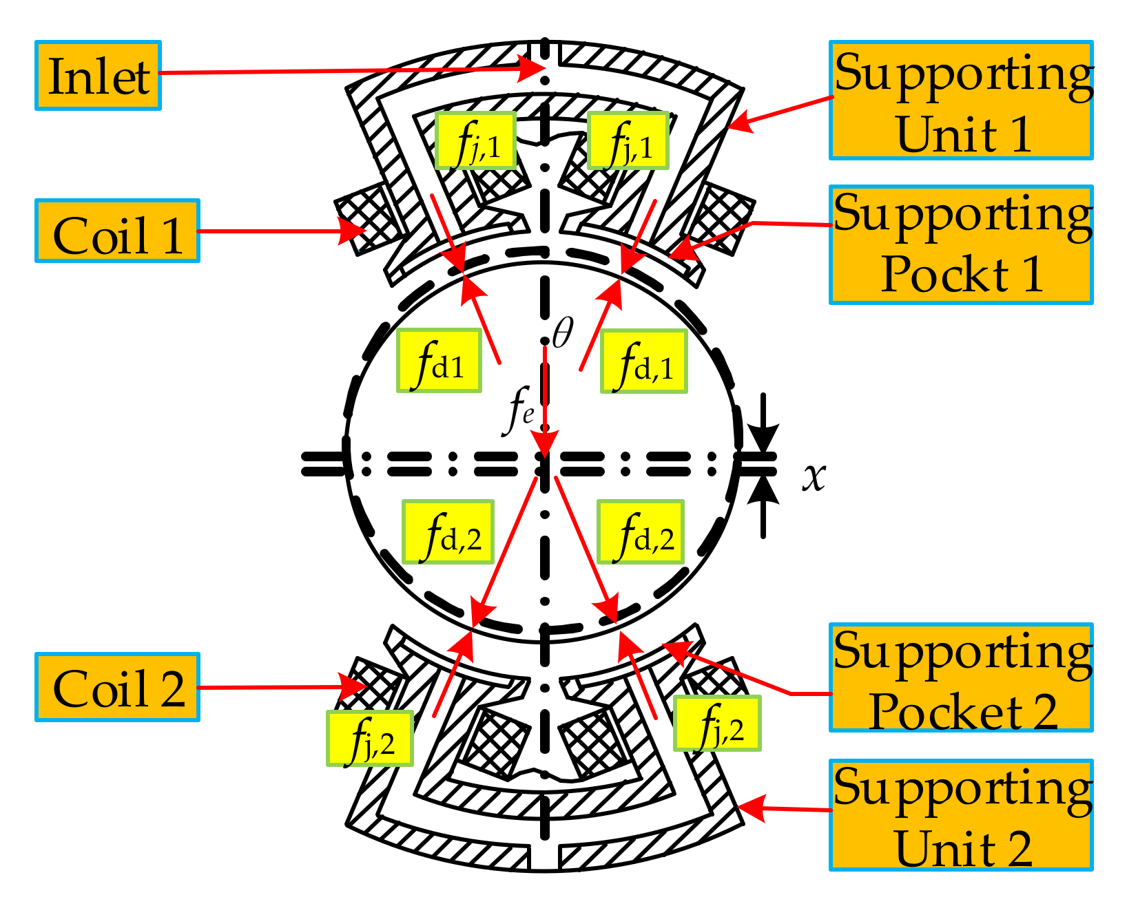
2.1. Mathematical Model of Supporting System in CFC Mode

The following assumptions are made for the electromagnetic suspension and hydrostatic bearing systems [17,18]:
(1)
The inertia force of the lubricant is ignored.
(2)
The viscosity–pressure characteristics of the liquid are ignored.
(3)
The coil flux leakage is ignored, considering that the coil flux is distributed uniformly in the magnetic circuit.
(4)
The magnetic resistance in the iron core and rotor is ignored, and the magnetic potential only acts on the air gap.
(5)
The magnetic hysteresis and eddy current of the magnetic materials are ignored.
(6)
The hydraumatic bearing surface is assumed as a rigid body.
(7)
The rotor gravity is ignored.
In the initial state, the hydrostatic force and the electromagnetic force of the upper and lower supporting cavities are equal, and the rotor is then suspended in an equilibrium position.
The vertical direction supporting system was used as the research object. It includes upper/lower supporting units and rotors, as shown in Figure 5.
The dynamics model was established [19], and the transfer function G(s) was obtained by Taylor expansion and Laplace transform:
G ( s ) = K i k p + k i / s + k d S m s 2 + K v , c S + K x , c K i = 2 µ 0 N 2 i 0 A x 0 2 cos θ K v , c = 4 µ A b A e B ¯ h 0 3 cos 2 θ K x , c = 2 µ 0 N 2 i 0 2 A x 0 3 cos θ + 6 q 0 µ A e B ¯ h 0 4 cos 2 θ
The design parameters of the MLDSB are shown in Table 1.
According to Equation (1), the dynamic model of the vertical supporting system under CFC was established as shown in Figure 6.

2.2. Step Response Analysis in CFC Mode

As shown in Figure 7, Figure 8 and Figure 9, step load was applied (time is 1 s, amplitude is 800 N) to the rotor, and the rotor displacement, regulating current, regulating flow, and supporting force were obtained.
Under the action of step load, the rotor displacement reached the reverse maximum of −24 μm at 1.6 s, and then it returned to the equilibrium position at 8 s with the action of combined regulation of hydrostatic and electromagnetic force. In the adjustment process, the static error of the rotor displacement was 0 μm, and the adjustment time was 7 s without overshoot, as shown in Figure 7.
According to Figure 8 and Figure 9, under the action of step load, the regulating current decreased to 2.5 A at 1.6 s initially and then gradually increased to a stable value of 6 A. At the same time, the electromagnetic force also decreased to 380 N at 1.6 s initially and then gradually increased to 800 N. The regulated flow gradually decreased from 0.25 L/min to 0 L/min. As the displacement of the rotor increased, liquid resistance increased, and the hydrostatic force reached the maximum value of 420 N at 1.6s. Finally, because of the decrease of liquid resistance and flow, the hydrostatic force decreased to 0 N.
After the rotor is returned to the balance position, the hydrostatic system no longer provides supporting force. The external load is carried only by electromagnetic force, and the supporting capacity and operation stability of the MLDSB can then be virtually reduced.

3. Numerical Simulation of the Rotor Impact-Rubbing Process under Electromagnetic Failure

Based on the above problems, the DCL control strategy was adopted to improve the stability and supporting stiffness of MLDSB.

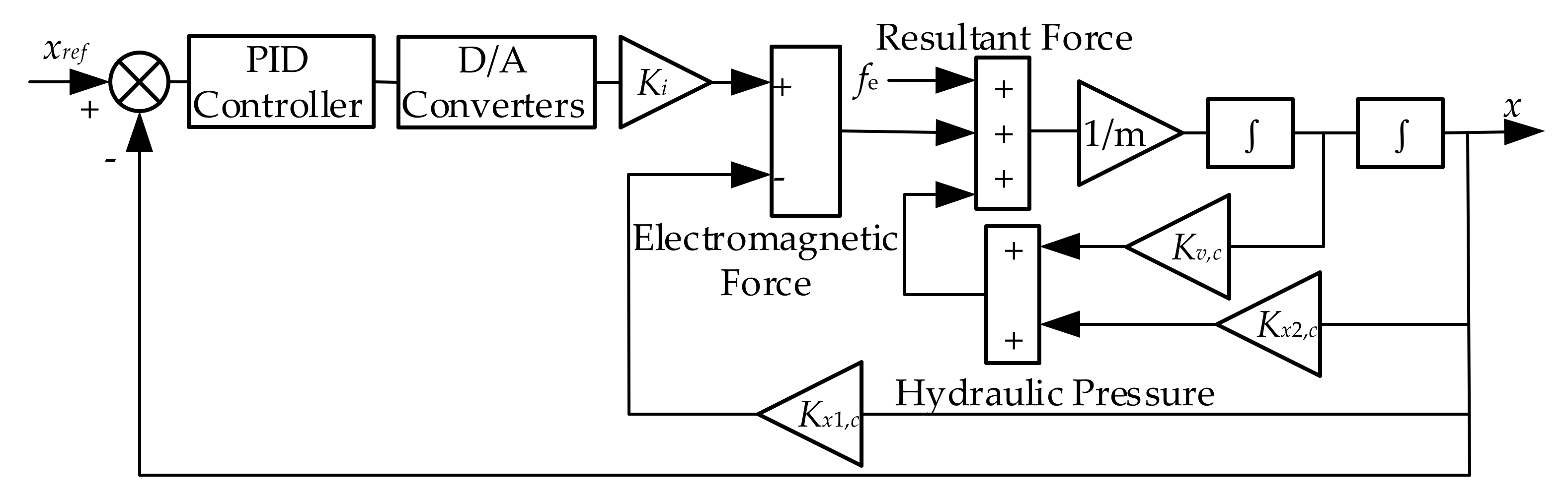
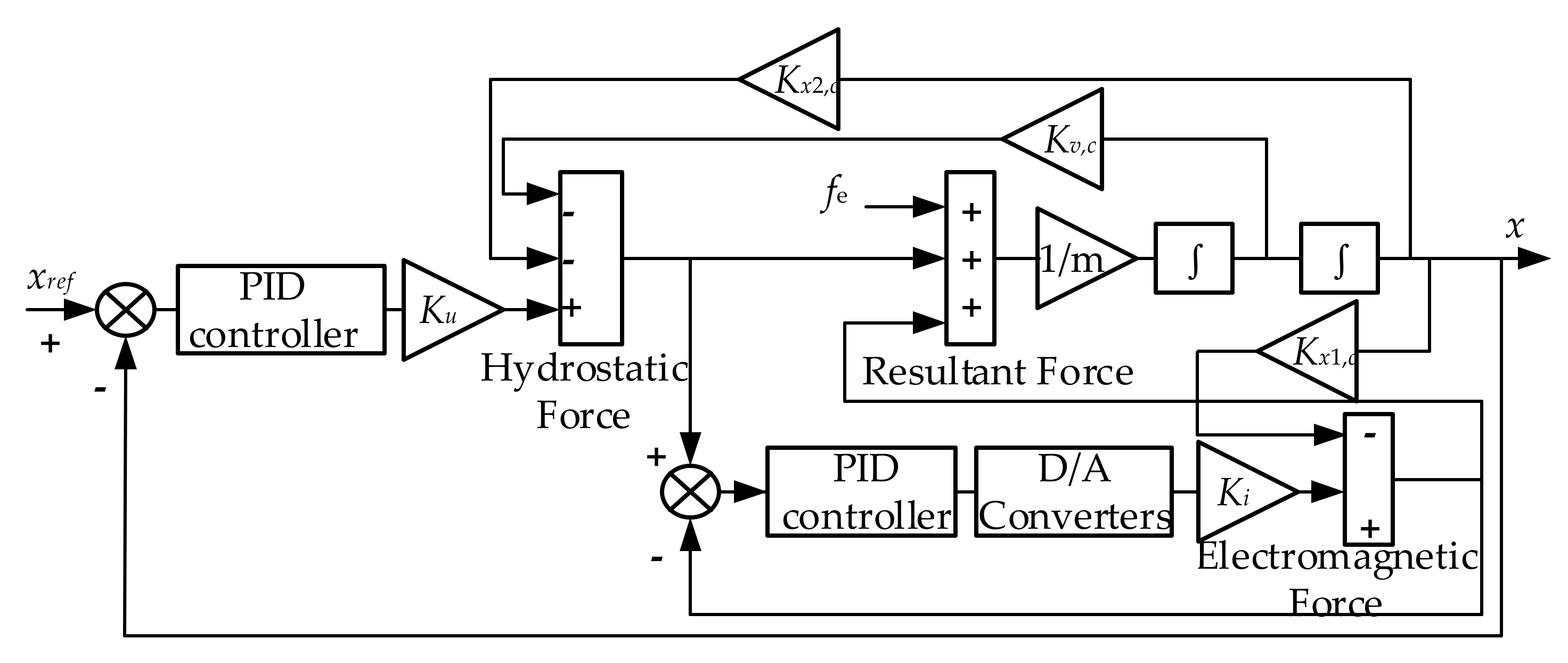
3.1. Mathematical Model of Supporting System under DCL Control

Taking the vertical support system under DCL control as the research object, the dynamic mathematical model G(s) was established:
G ( s ) = K u k p + k i / s + k d S m s 2 + 2 K v , v S + K x , v K u = 4 µ k A e B ¯ h 0 3 cos θ K v , v = 4 µ A b A e B ¯ h 0 3 cos 2 θ K x , v = 2 µ 0 N 2 i 0 2 A x 0 3 cos θ + 6 u 0 µ k A e B ¯ h 0 4 cos 2 θ
According to Equation (2), a simulation model of the vertical system in DCL mode was established, as shown in Figure 10.

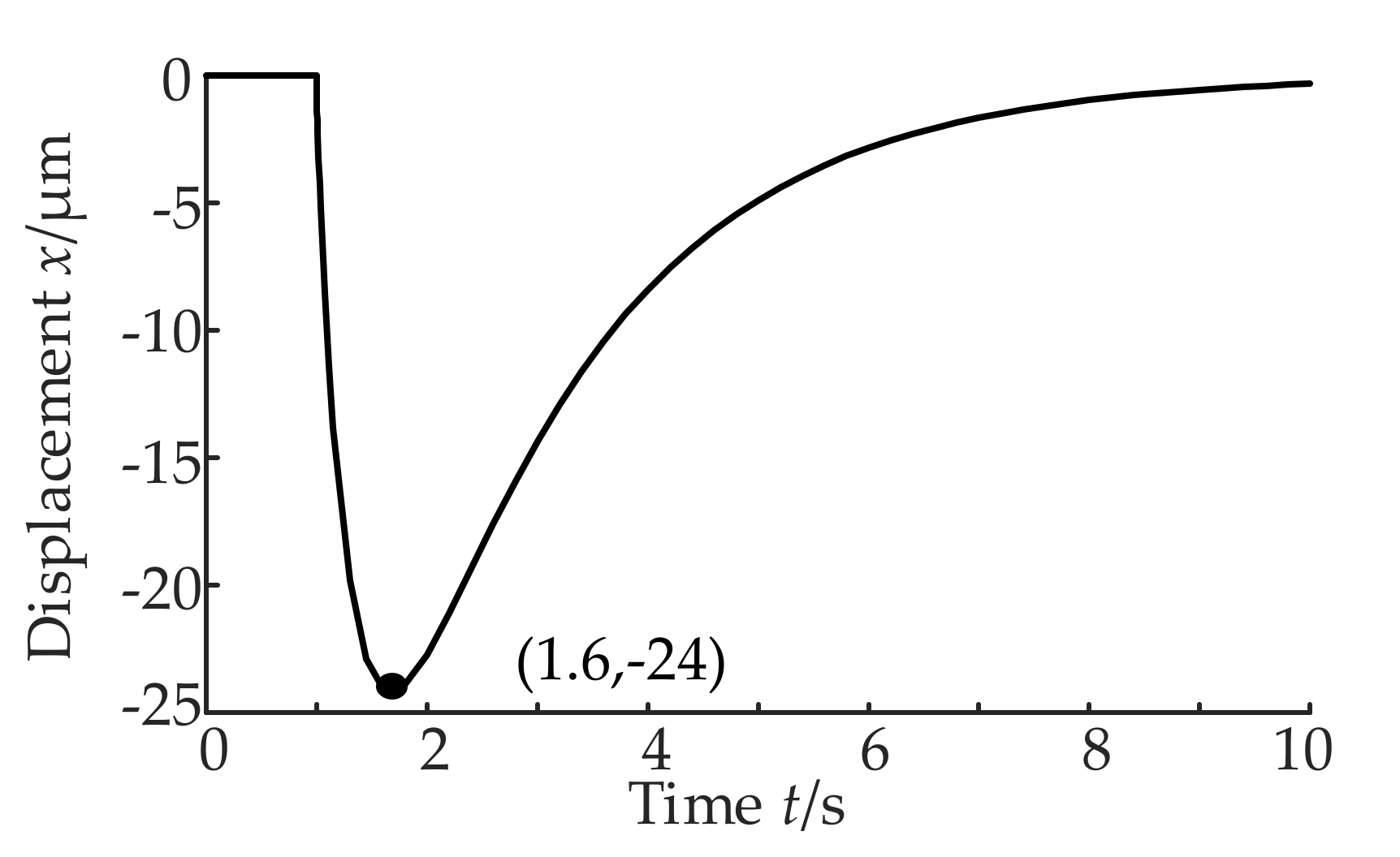
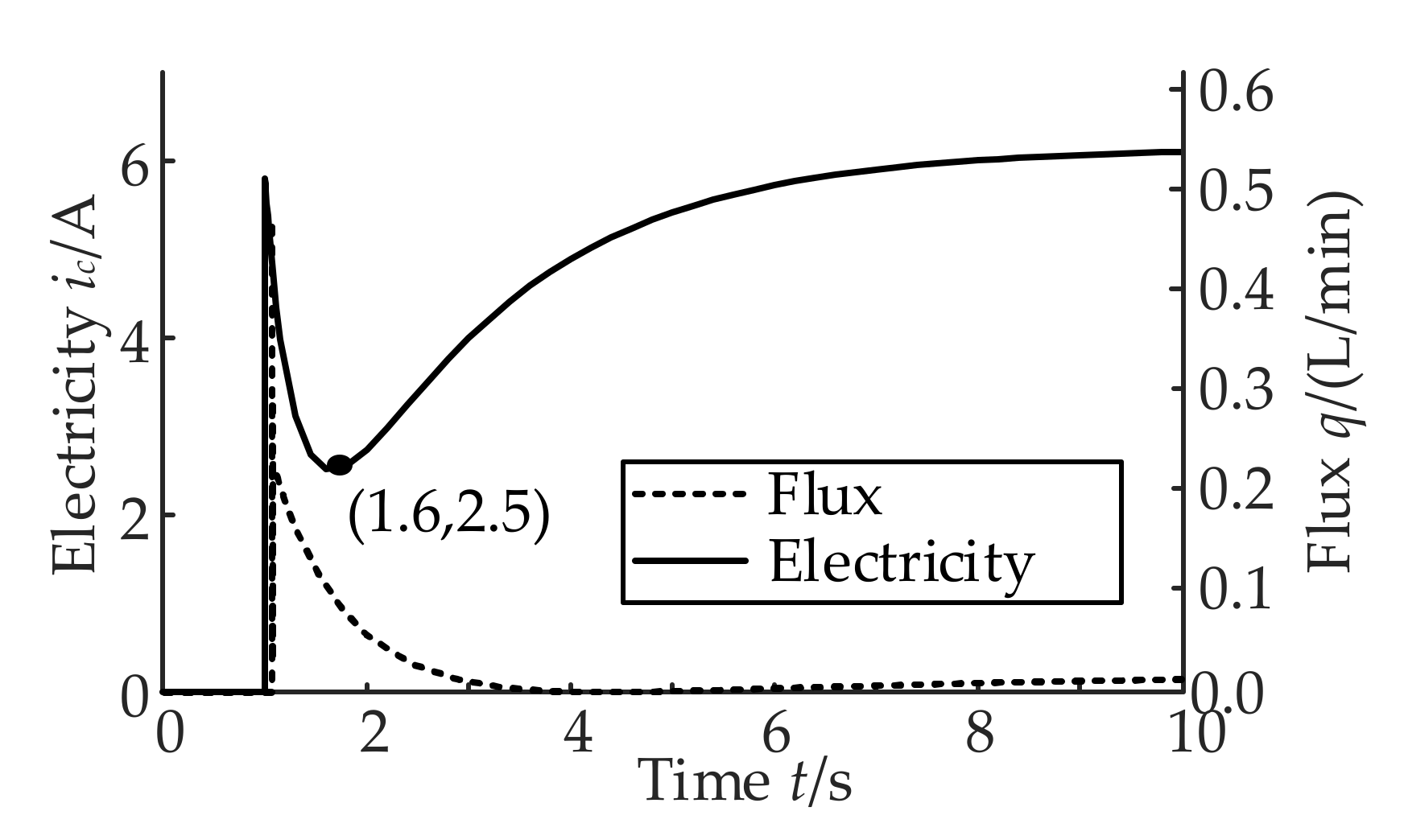
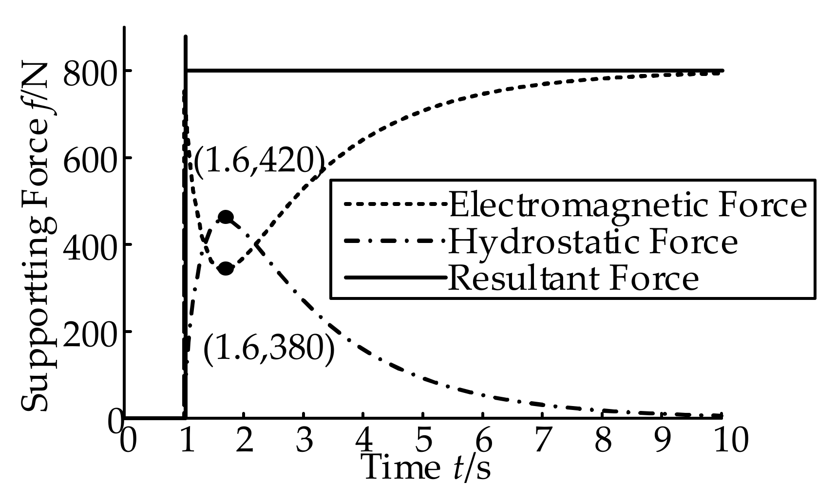
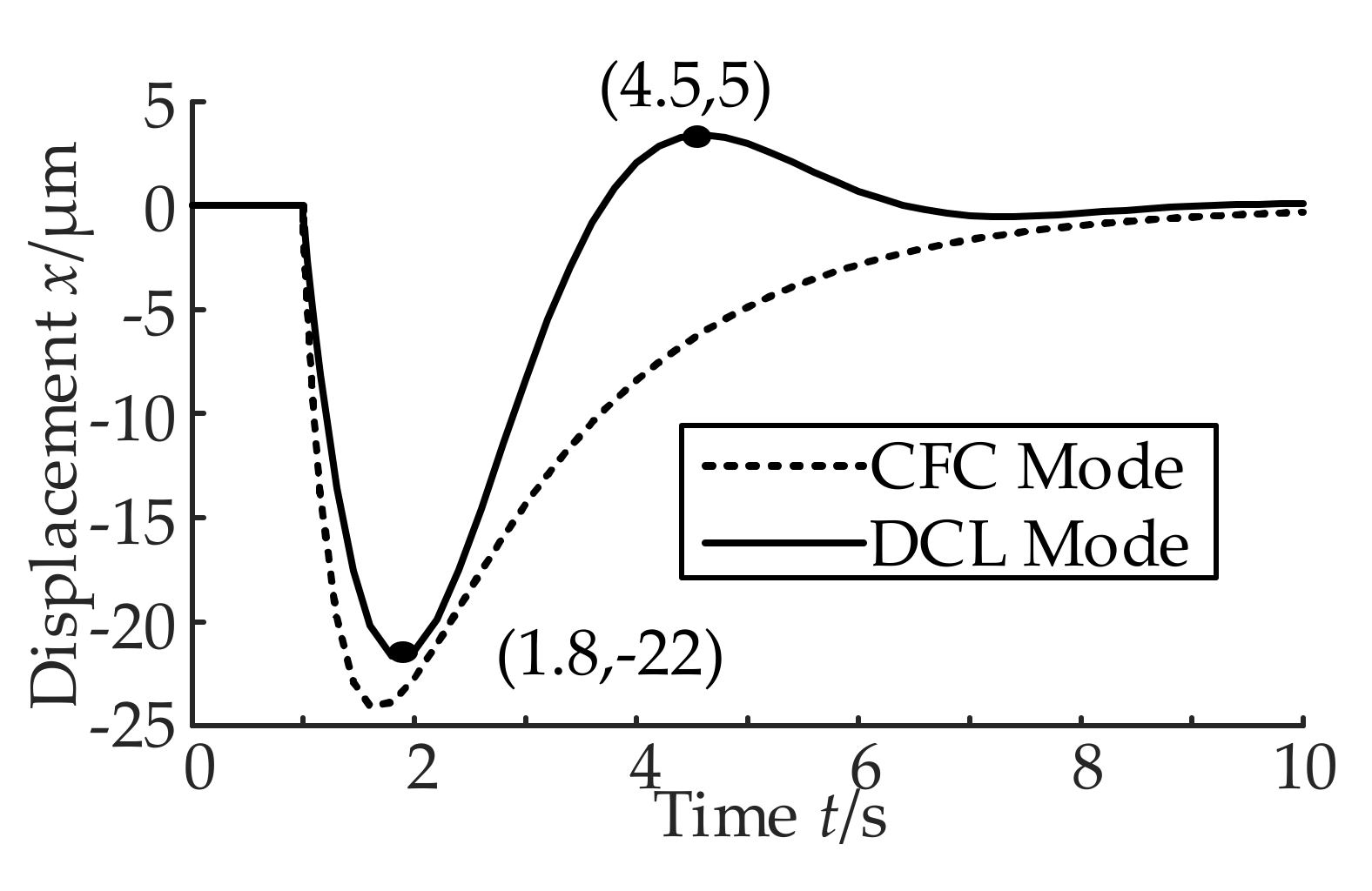
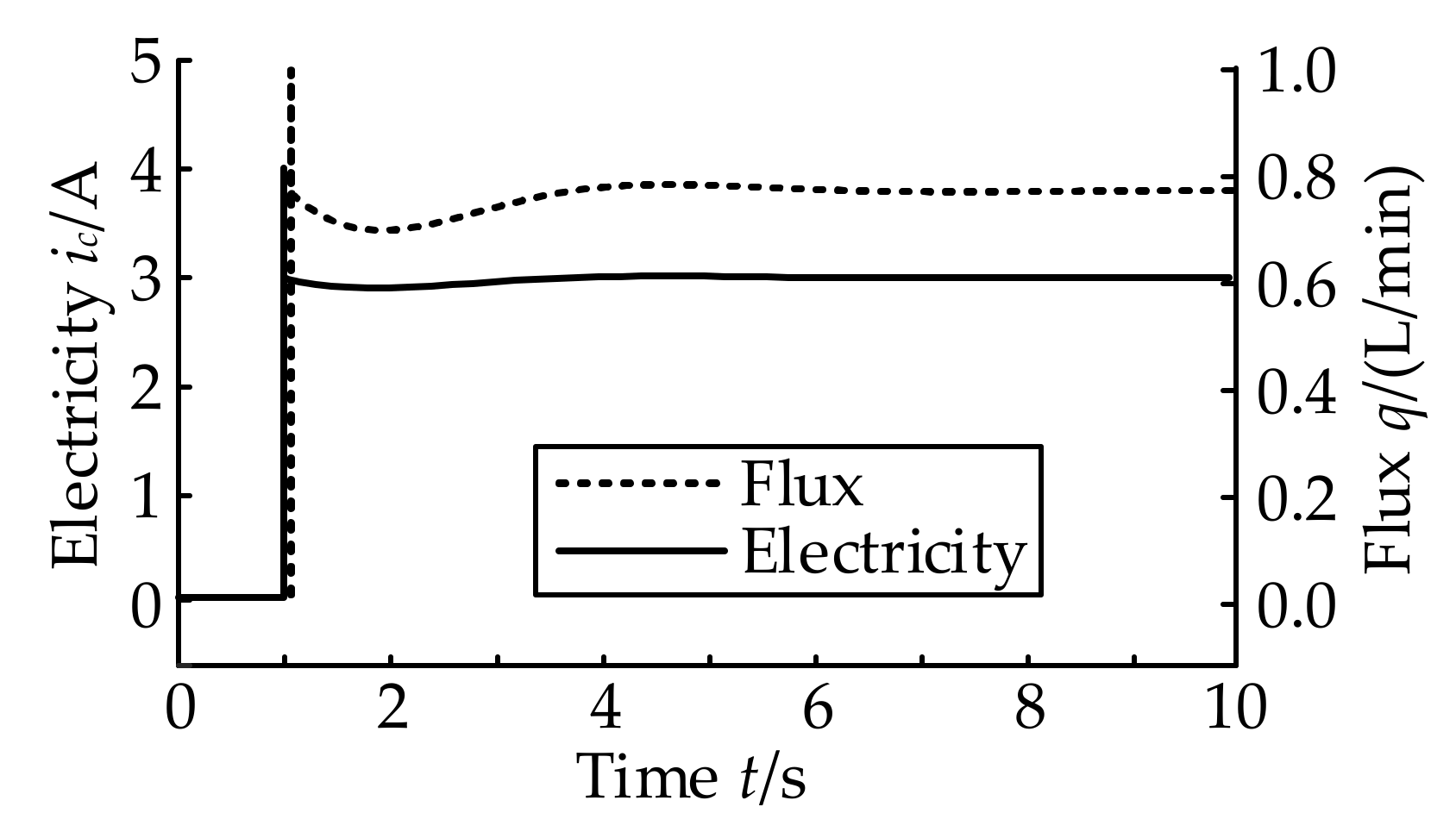
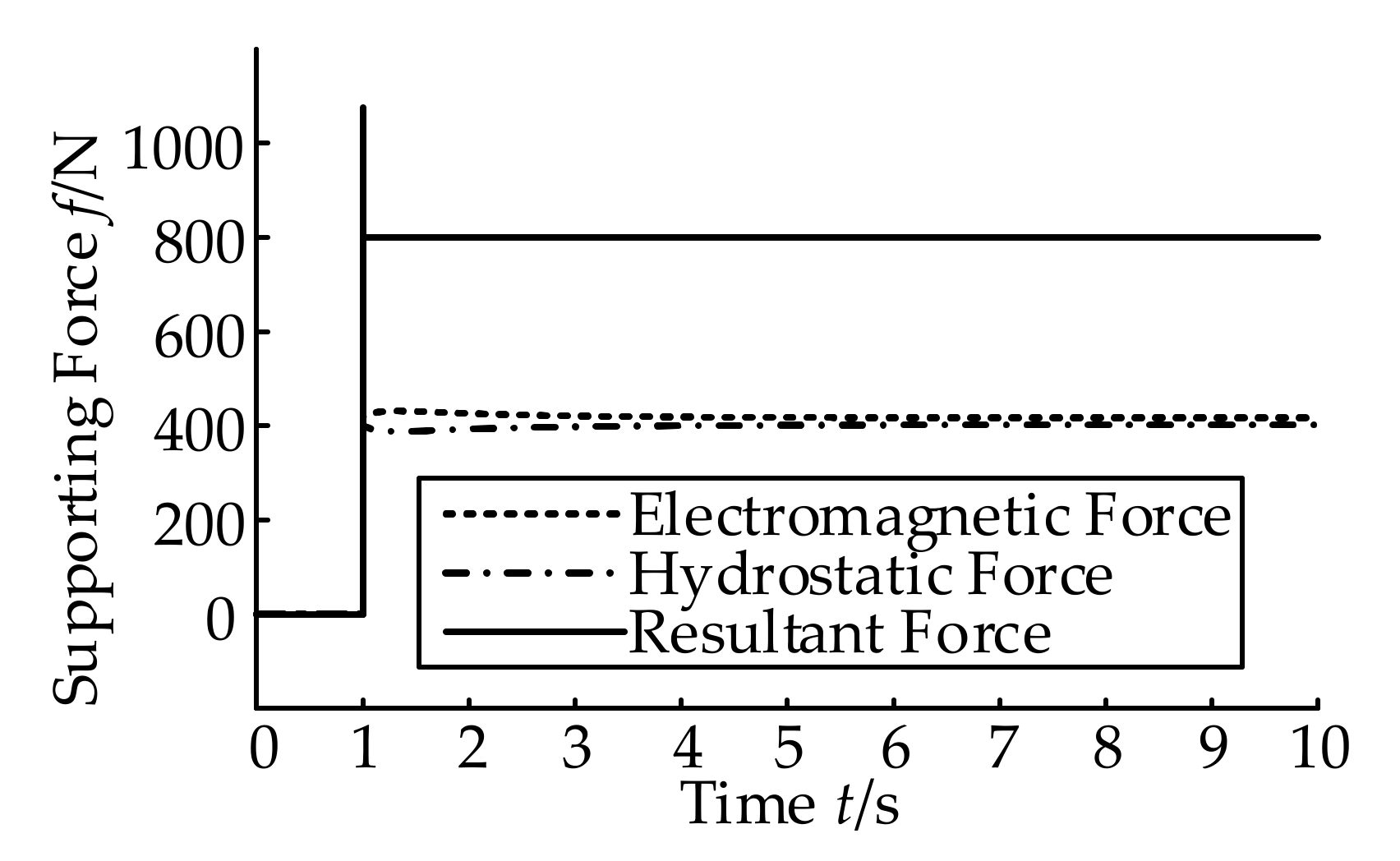
3.2. Simulation Analysis in DCL Mode under Step Response

Similarly, as shown in Figure 11, step load was applied (time is 1 s, amplitude is 800 N) to the rotor to obtain the rotor displacement under DCL control. The current/flow and the supporting force are shown in Figure 12 and Figure 13.
As shown in Figure 11, the rotor reached a reverse maximum of −22 μm at 1.8 s, then crossed the equilibrium position and reached a forward maximum of 5 μm at 4.5 s because of the combined regulation of the hydrostatic force and electromagnetic force, and finally stabilized at the equilibrium position at 6 s with an error of 0 μm.
According to Figure 12 and Figure 13, the current of the electromagnetic system in the DCL control mode increased to 3 A and gradually reached stability. The electromagnetic force reached a stable value of 400 N at 4 s. After a period of adjustment, the flow of the hydromantic system was stable at 0.8 L/min at 4 s, and the hydrostatic force reached a stable value of 400 N. The hydrostatic force was equal to the electromagnetic force.
According to Figure 11, compared with that under CFC, the rotor displacement under DCL control mode produced overshoot, but the adjustment time was shorter.
Comparing Figure 9 with Figure 13, after the rotor returns to the equilibrium position, the electromagnetic force and the hydrostatic force always maintain a certain proportion so as to achieve the maximum load output of the electromagnetic force and hydrostatic force, and the supporting capacity and operation stability of the MLDSB are improved.

4. Analysis of Dynamic and Static Characteristics in Different Modes

In order to further explore the dynamic and static characteristics under different control modes, the static stiffness j0 and steady-state error ess were taken as static characteristics [20,21]. The dynamic stiffness J, the adjustment time ts, and the amplitude–phase characteristic curve were taken as dynamic characteristics [22,23], and the influence of the initial current i0, the initial flow q0, the proportional coefficient kp, and the differential coefficient kd of the PID controller on the dynamic and static characteristics of the system were explored.

4.1. Index of Characteristic

① Static stiffness represents the ability of the MLDSB to resist deformation under vertical load [24], which can be expressed as:
j 0 = 2 µ 0 N 2 i 0 2 A cos θ + 6 q 0 µ A e cos 2 θ + 4 k p µ A b A e h 0 x 0 3 cos 2 θ m B ¯ h 0 4 x 0 3   CFC 2 µ 0 N 2 i 0 2 A cos θ + 12 u 0 µ k A e cos 2 θ + 4 k p µ A b A e h 0 x 0 3 cos 2 θ m B ¯ h 0 4 x 0 3   DCL  
② Steady-state error refers to the deviation of the MLDSB when the system reaches a new equilibrium state [25], which can be expressed as follows:
e s s ( ) = m k d µ 0 N 2 i 0 A x 0 B ¯ h 0 4 µ 0 N 2 i 0 2 A B ¯ h 0 4 + 6 q 0 µ A e x 0 3 cos θ + 4 k p µ A b A e 0 x 0 3 cos 2 θ h   CFC 4 m k d µ A b A e x 0 3 h 0 cos θ µ 0 N 2 i 0 2 A B ¯ h 0 4 + 6 u 0 µ k A e x 0 3 cos θ + 4 k p µ A b A e 0 x 0 3 cos 2 θ h   DCL
③ Dynamic stiffness represents the ability of the MLDSB to resist external load in the frequency domain, which is equal to the reciprocal of the system frequency characteristics [26,27] and can be expressed as:
J = 2 µ 0 N 2 i 0 2 A cos θ x 0 3 + 6 q 0 µ A e cos 2 θ B ¯ h 0 4 + 4 k p µ k A e B ¯ h 0 3 m ω 2 2 + 4 k d µ k A e cos θ B ¯ h 0 3 2   CFC 4 µ 0 N 2 i 0 2 A cos θ x 0 3 + 6 k u µ A e cos 2 θ B ¯ h 0 4 + 4 k p µ k A e B ¯ h 0 3 m ω 2 2 + 8 k d µ k A e cos θ B ¯ h 0 3 2   DCL  
where external loading frequency ω = 100 Hz.
Since the system in the double closed-loop control mode is a second-order overdamped system, the rise time of the MLDSB was selected as the adjustment time, which can be expressed as follows:
t s = m x 0 3 2 µ 0 N 2 i 0 2 A + m h 0 4 6 q µ A e cos 2 θ + 1.5 m µ A b A e cos θ µ 0 N 2 i 0 2 A B ¯ h 0 3 x 0 3 + 3 q µ A e cos 2 θ h 0 + 4 µ A b A e cos 2 θ B ¯ 2 2 µ 0 N 2 i 0 2 A cos θ m x 0 3 h 0 4 + 6 q µ A e cos 2 θ m B ¯ h 0 8 3 2 CFC m x 0 3 2 µ 0 N 2 i 0 2 A + m h 0 4 12 q µ A e cos 2 θ + 1.5 m µ A b A e cos θ µ 0 N 2 i 0 2 A B ¯ h 0 3 x 0 3 + 6 q µ A e cos 2 θ h 0 + 4 4 µ A b A e cos 2 θ B ¯ 2 2 µ 0 N 2 i 0 2 A cos θ m x 0 3 h 0 4 + 6 q µ A e cos 2 θ m B ¯ h 0 8 3 2 DCL

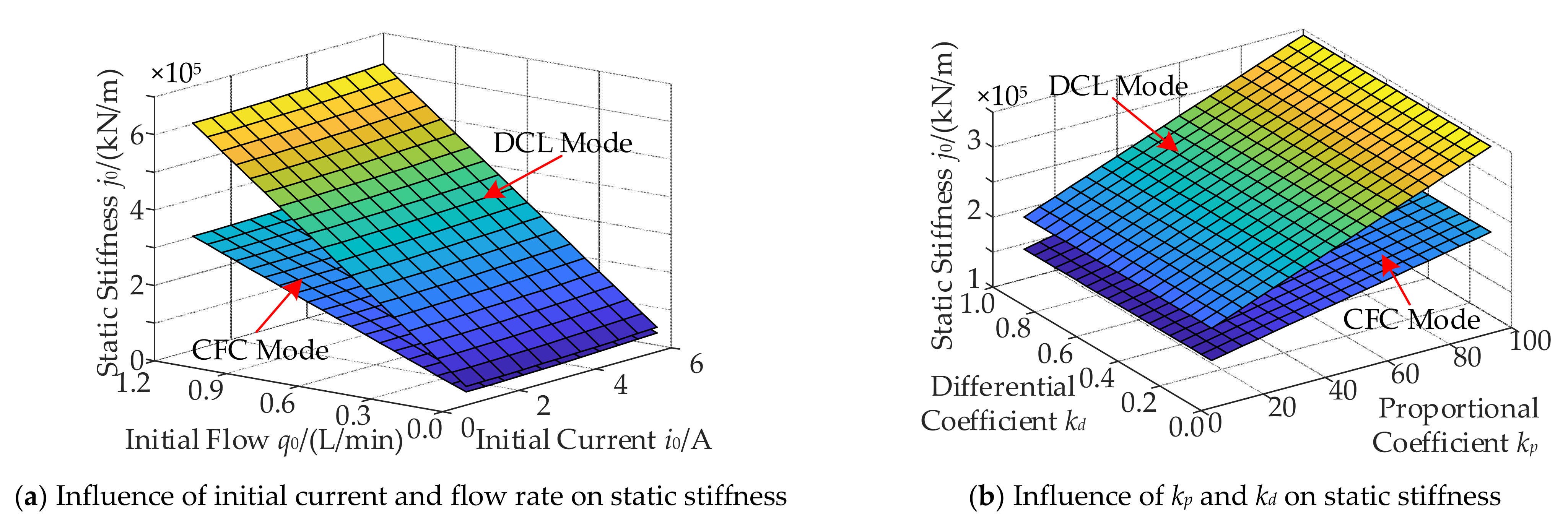
4.2. Variation Law of Static Stiffness with Parameters

① The static stiffness of the MLDSB under the two control modes can be obtained by changing initial current i0 and initial flow q0 as shown in Figure 14a.
In CFC mode, as the initial flow increased from 0.06 L/min to 1.2 L/min, the static stiffness increased from 0.2 × 10⁵ kN/m to 3 × 10⁵ kN/m. As the initial current increased from 1 A to 6 A, the static stiffness increased from 0.8 × 10⁵ kN/m to 1.5 × 10⁵ kN/m, and the initial current had little impact on the static stiffness.
In DCL control mode, with the increase of initial flow, the static stiffness increased from 0.3 × 10⁵ kN/m to 6 × 10⁵ kN/m. When the initial flow was 0.6 L/min, the static stiffness increased from 2 × 10⁵ kN/m to 3 × 10⁵ kN/m. The static stiffness increased more obviously in DCL control mode.
② The static stiffness of the MLDSB under the two control modes can be obtained by changing the proportional coefficient kp and the differential coefficient kd, as shown in Figure 14b.
In CFC mode, as the proportional coefficient kp increased from 10 to 100, the static stiffness increased from 1 × 10⁵ kN/m to 2.5 × 10⁵ kN/m. However, the static stiffness remained the same when kd changed. Therefore, the static stiffness of the MLDSB cannot be improved by increasing kd.
In DCL mode, when kp increased gradually, the static stiffness increased from 1.6 × 10⁵ kN/m to 3.2 × 10⁵ kN/m. However, when kd gradually increased from 0.1 to 1.0, the static stiffness did not change.

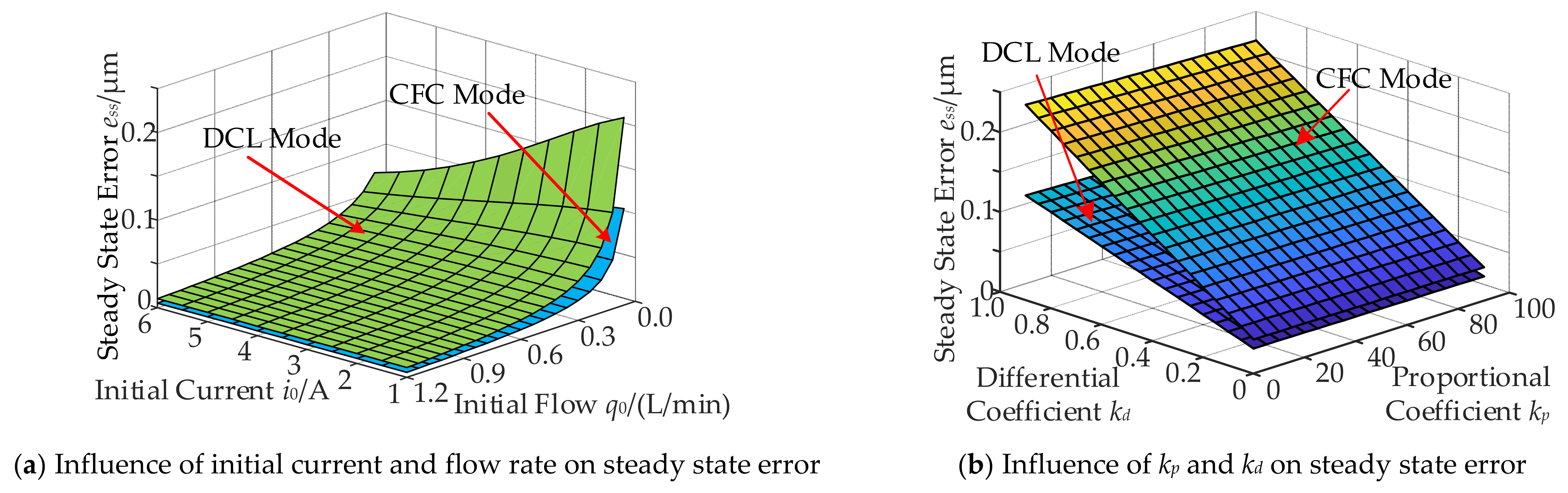
4.3. Variation Law of Steady-State Error with Parameters

① The steady-state error under the two control modes can be obtained by changing the initial current i0 and the initial flow q0, as shown in Figure 15a:
In CFC mode, the steady-state error of the MLDSB decreased gradually with the increase of the initial flow. When the initial current was 5 A, the initial flow increased gradually from 0.06 L/min to 1.2 L/min, and the steady-state error decreased from 0.07 μm to 0.01 μm. With the increase of initial current, the steady-state error also decreased gradually, and initial flow had a full effect on the steady-state error.
In DCL control mode, the initial flow and current had the same influence on the MLDSB as in CFC mode. In addition, the steady-state error mode was smaller than that in CFC mode.
② The steady-state error of the MLDSB can be obtained by changing the proportional coefficient kp and the differential coefficient kd, as shown in Figure 15b.
The variation of the steady-state error with parameters in DCL mode was the same as that in CFC mode. However, the steady-state error in DCL mode was smaller than that in CFC mode. When kd was 0.5, the steady-state error of the MLDSB in CFC mode decreased from 0.15 μm to 0.1 μm, with kp increasing from 10 to 100, while the steady-state error decreased from 0.06 μm to 0.04 μm in DCL control mode. However, simply increasing kp cannot eliminate the steady-state error. When kd increased from 0.1 to 1.0, the steady-state error increased gradually from 0.02 μm to 0.2 μm in CFC mode and from 0.02 μm to 0.12 μm in DCL mode.

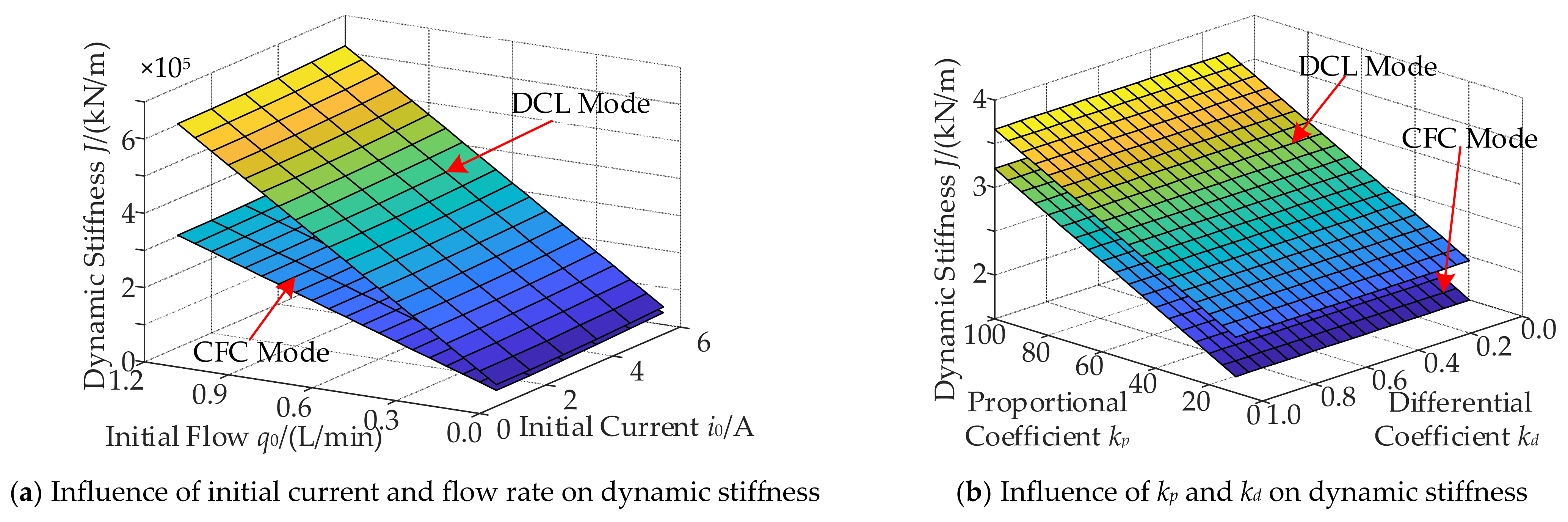
4.4. Variation Law of Dynamic Stiffness with Parameters

① The dynamic stiffness under the two control modes can be obtained by changing the initial current i0 and the initial flow q0, as shown in Figure 16a.
When the initial current was 2 A and initial flow increased from 0.06 L/min to 1.2 L/min, the dynamic stiffness in CFC mode increased from 0.5 × 10⁵ kN/m to 3 × 10⁵ kN/m, while the dynamic stiffness in DCL mode increased from 0.5 × 10⁵ kN/m to 6 × 10⁵ kN/m. Thus, the initial flow had a stronger effect on the dynamic stiffness in DCL mode. With the increase of initial current, the dynamic stiffness in CFC mode increased from 0.8 × 10⁵ kN/m to 1.2 × 10⁵ kN/m, while the dynamic stiffness in DCL mode increased from 1.5 × 10⁵ kN/m to 2 × 10⁵ kN/m.
Therefore, the dynamic stiffness of the MLDSB in DCL mode is greater than that in CFC mode, and it is sensitive to initial flow in the two control modes.
② The dynamic stiffness under the two control modes can be obtained by changing the proportional coefficient kp and the differential coefficient kd, as shown in Figure 16b.
With the increase in the proportional coefficient kp and the differential coefficient kd, the dynamic stiffness under the two control modes improved. When kd was 0.5, with kp increasing from 10 to 100, the dynamic stiffness increased from 1.5 × 10⁵ kN/m to 3.2 × 10⁵ kN/m in CFC mode. In DCL mode, the dynamic stiffness increased from 2.0 × 10⁵ kN/m to 3.7 × 10⁵ kN/m. The proportional coefficient kp had a full effect on the dynamic stiffness.

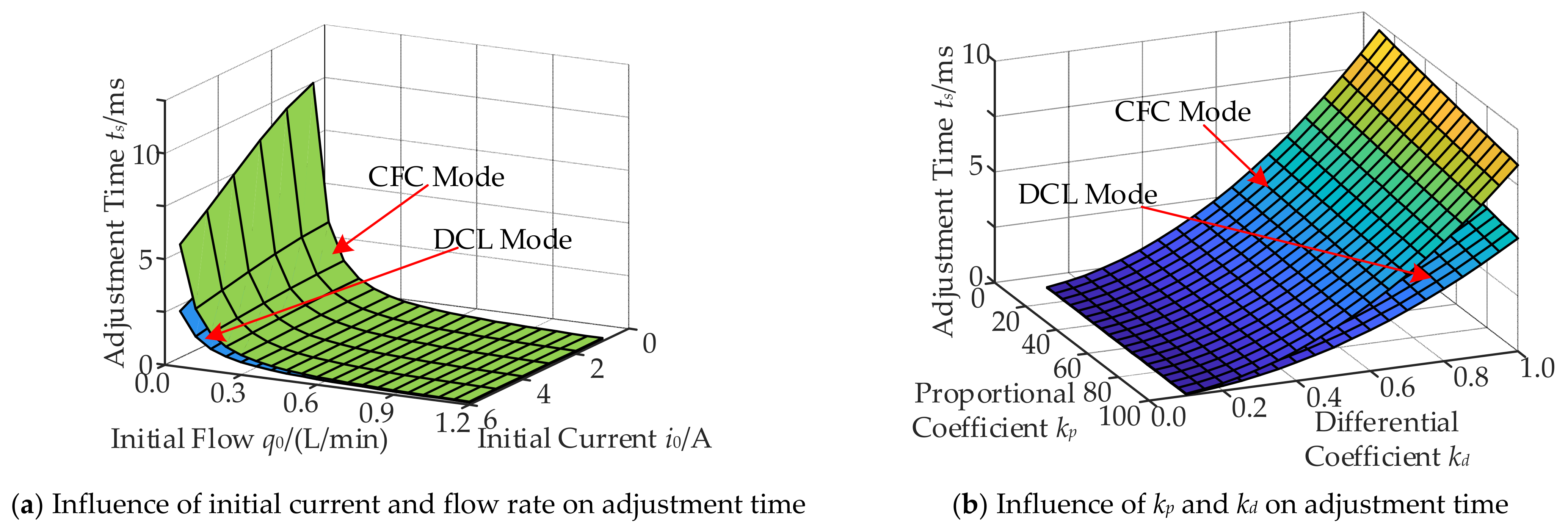
4.5. Variation Law of Adjustment Time with Parameters

① The adjustment time of the MLDSB under the two control modes can be obtained by changing the initial current i0 and the initial flow q0, as shown in Figure 17a.
With the increase in initial flow and initial current, the adjustment time decreased gradually under the two modes. When the initial flow was 0.3 L/min, with the initial current increasing from 1 A to 6 A, the adjustment time in CFC mode gradually decreased from 1.6 ms to 0.6 ms, while it decreased from 1 ms to 0.4 ms in DCL mode. When the initial current was 3 A, with an increase in the initial flow, the adjustment time in CFC mode decreased from 5 ms to 0.4 ms, while it decreased from 1.5 ms to 0.3 ms in DCL mode. Therefore, the adjustment time in DCL mode is shorter than that in CFC mode.
② The adjustment time of the MLDSB under two control modes can be obtained by changing the proportional coefficient kp and the differential coefficient kd, as shown in Figure 17b.
With the increase in the proportional coefficient kp and the decrease in the differential coefficient kd, the adjustment time of the MLDSB under the two control modes decreased, but the decrease was more obvious in CFC mode. When kd was 0.5, with kp increasing from 10 to 100, the adjustment time in CFC mode decreased from 4 ms to 2 ms, while it decreased from 1.6 ms to 0.8 ms in DCL mode. When kp was 50, with kd increasing from 0.1 to 1.0, the adjustment time in CFC mode increased from 1 ms to 4 ms, and it increased from 0.6 ms to 2 ms in DCL mode.
Thus, with the same proportional coefficient kp and differential coefficient kd, the adjustment time in DCL mode is shorter than that in CFC mode.

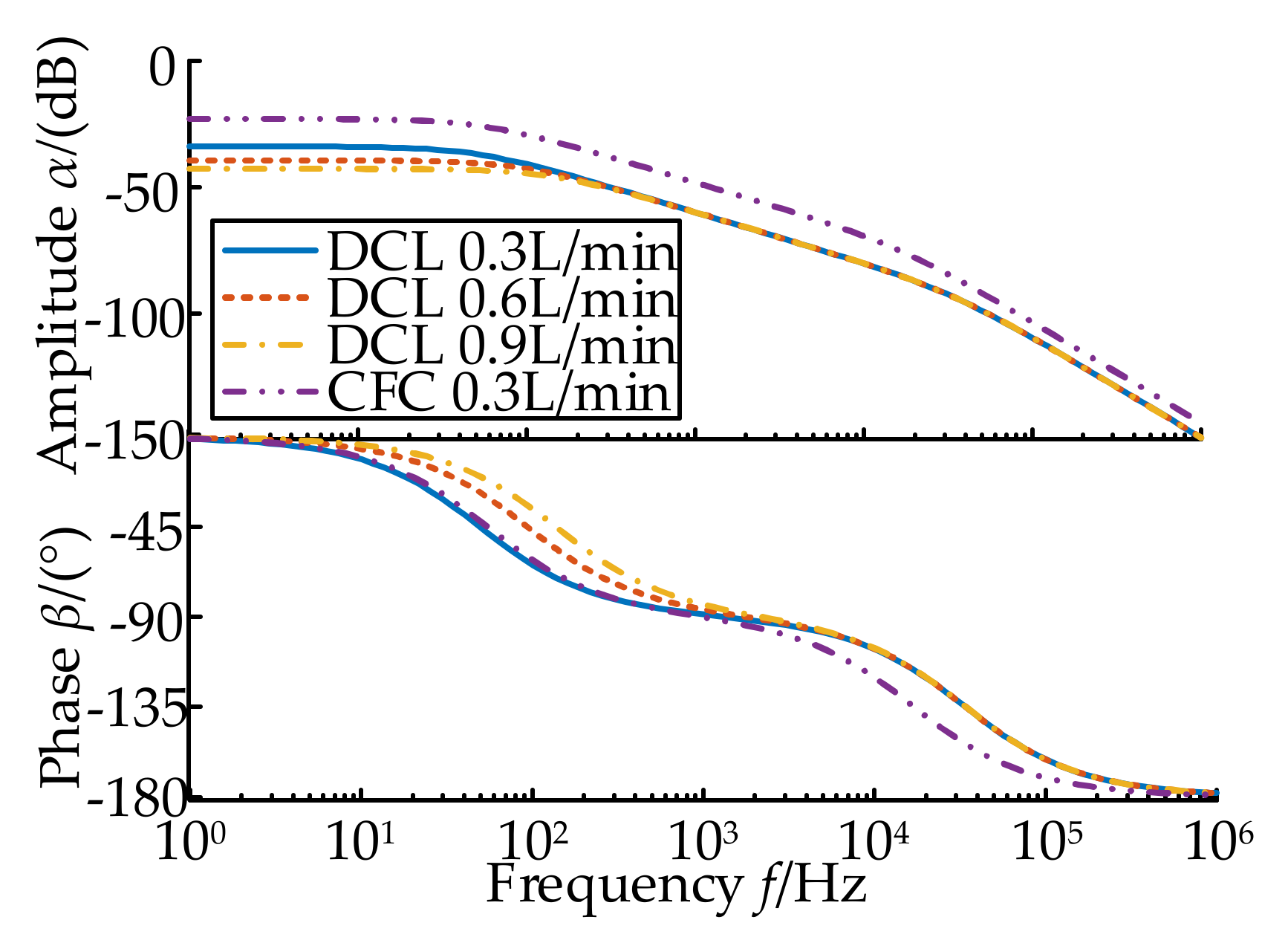
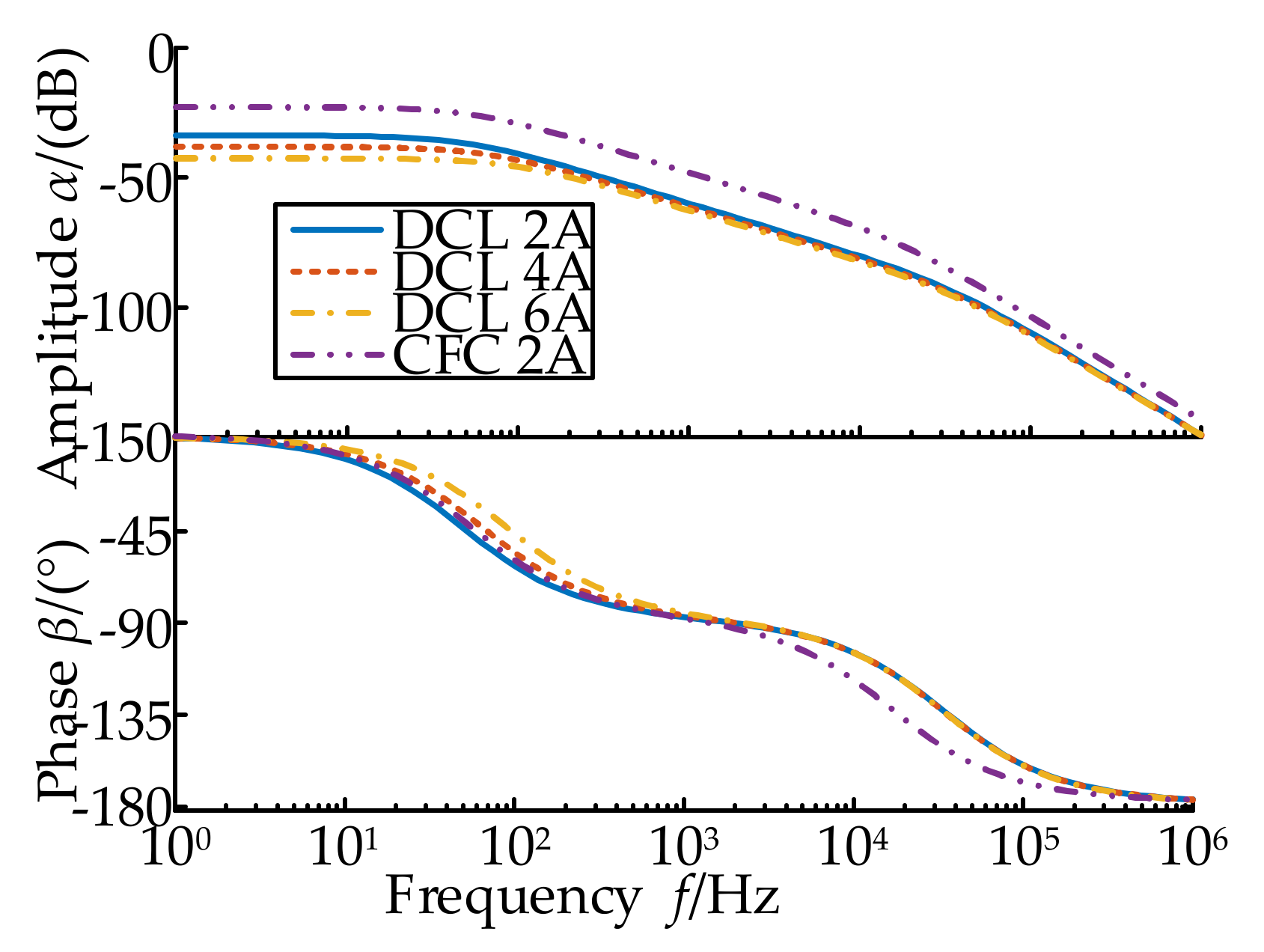
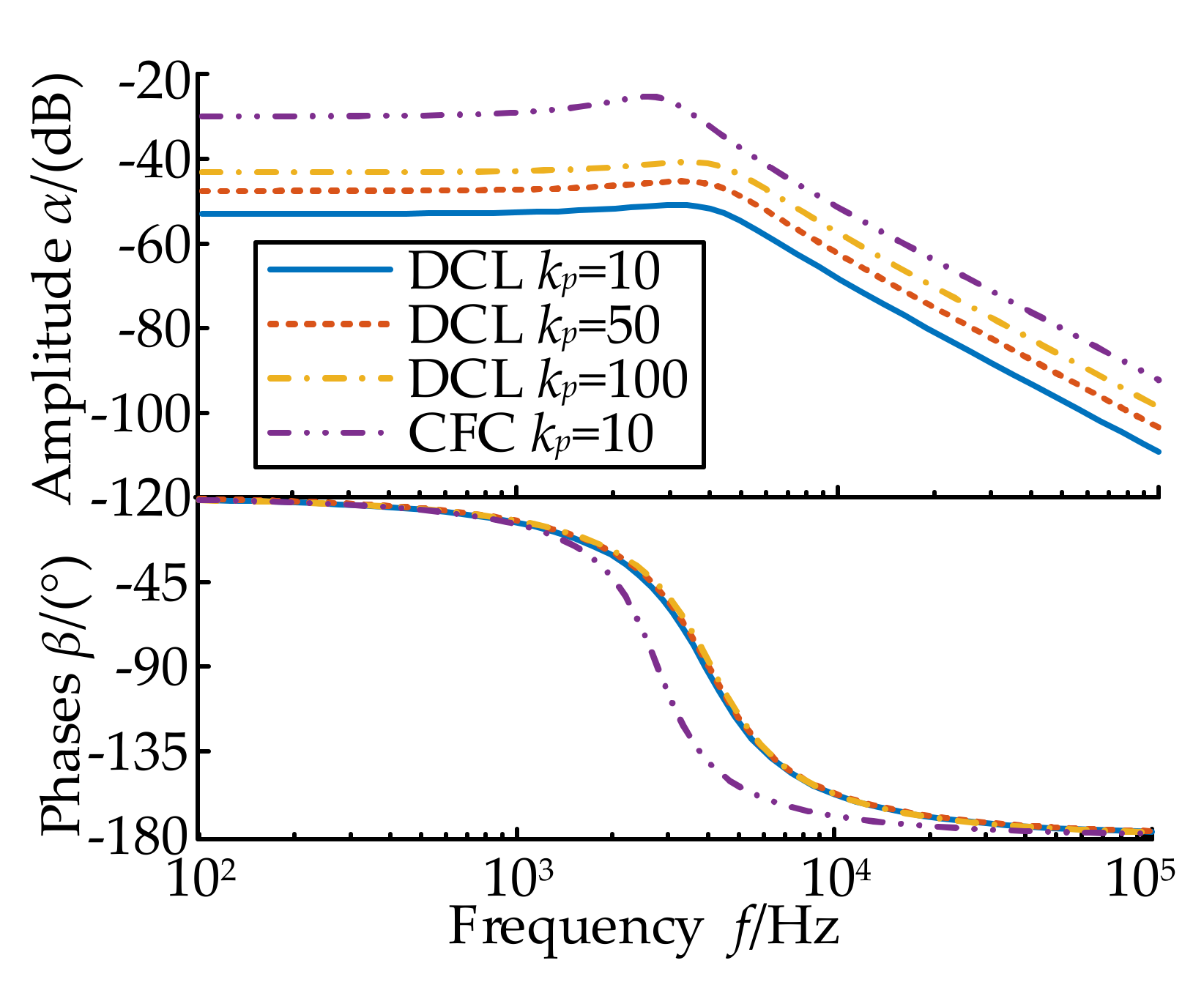
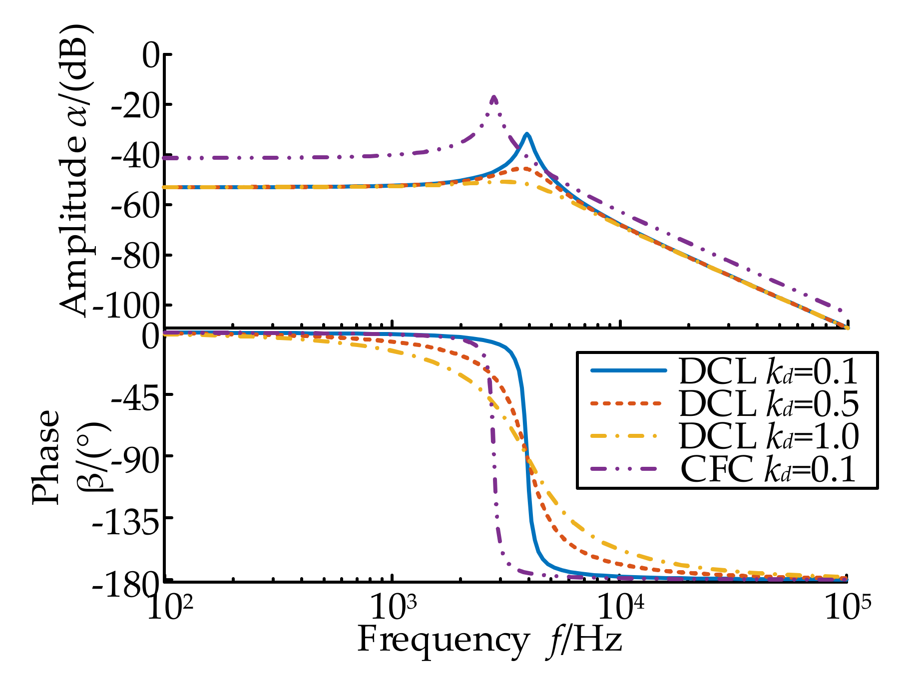
4.6. Variation Law of Amplitude–Phase Curve with Parameters

① The amplitude and phase characteristic curve of the MLDSB under the two modes can be obtained by changing the initial current i0 and the initial flow q0, as shown in Figure 18 and Figure 19.
According to Figure 18 and Figure 19, within the range of 100–102 Hz, the amplitude in DCL mode was less than that in CFC mode, and the MLDSB had stronger low-frequency disturbance immunity. In the range of 102–104 Hz, the amplitude slope in DCL mode was closer to −20 dB/dec, and the MLDSB had better robustness [28,29]. In the range of 104–106 Hz, the amplitude in DCL mode was smaller, and the MLDSB had a better high-frequency noise suppression ability. In the range of 100–103 Hz, the phase angle in DCL mode coincided with that in CFC mode. In the range of 103–106 Hz, the phase angle in DCL mode was greater than that in CFC mode.
In DCL mode, in the range of 100–102 Hz, the amplitude of the curve decreased gradually with an increase in the initial current i0 and the initial flow q0, and the low-frequency disturbance resistance increased [30]. In the range of 102–106 Hz, the amplitude characteristic curves were equal, and the robustness and high-frequency noise suppression effect of the MLDSB remained the same with an increase in initial current and flow.
In the range of 100–103 Hz, with an increase in the initial current i0 and the initial flow q0, the phase angle increased. In addition, in the range of 103–106 Hz, the phase–frequency characteristic curves coincided with those under different currents.
② The amplitude and phase characteristic curve can be obtained by changing the proportional coefficient kp and the differential coefficient kd, as shown in Figure 20 and Figure 21.
The proportional coefficient kp mainly affects the stability of MLDSB. With an increase in kp, the amplitude–frequency curve increased, causing the stability margin to decrease gradually and the stability to weaken accordingly. The phase frequency characteristic curves coincided with different kp, and the phase angle remained the same with an increase in the proportional coefficient.
However, the differential coefficient kd mainly affects the damping characteristics. In the range of 1 × 10²–2 × 10³ Hz and 1 × 10⁴–1 × 10⁵ Hz, the amplitude–frequency curves under different kd were equal, and the differential coefficient kd had no influence on the MLDSB. In the range of 2 × 10³–1 × 10⁴ Hz, with the increase of the differential coefficient kd, the peak value of the turning point gradually decreased and flattened out, and the damping gradually increased. The phase–frequency characteristic curves basically coincided with those in the ranges of 102–103 Hz and 104–105 Hz. By contrast, in the range of 103–104 Hz, with a gradual increase in kd, the phase–frequency characteristic curve gradually slowed down.

5. Conclusions

(1)
In DCL mode, the displacement was smaller and the adjustment time was shorter, and the hydrostatic force and electromagnetic force retained a certain proportion.
(2)
Increasing the initial current and the initial flow can improve the dynamic and static characteristics of the MLDSB. However, as the oil film thickness is smaller than the electromagnetic air gap, the initial flow has a stronger effect on the dynamic and static characteristics.
(3)
In DCL mode, the static and dynamic stiffnesses are greater and the adjustment time is shorter, but the steady-state error is larger than that in CFC mode.
(4)
Increasing kp can improve the stiffness and reduce the adjustment time and steady-state error. However, excessive kp will lead to instability of the MLDSB. The steady-state error, adjustment time, and damping increased with an increase in kd, but kd had little effect on the stiffness of the MLDSB.

Author Contributions

Conceptualization, J.Z.; methodology, Y.W., G.D.; software, Y.W.; validation, X.M. and S.L.; formal analysis, X.M.; writing—original draft preparation, Y.W.; writing—review and editing, J.Z. and Y.W.; supervision, D.G. All authors have read and agreed to the published version of the manuscript.

Funding

This work was supported by the National Nature Science Foundation of China (No. 52075468), a general project of the Natural Science Foundation of Hebei Province (No. E2020203052), the Scientific Research Fund Project of Colleges and Universities in Hebei Province (QN202013), and the Open Project Funding of Fluid Power Transmission Control Laboratory of Yanshan University.

Data Availability Statement

Not applicable.

Conflicts of Interest

The authors declare no conflict of interest.

References

  1. Zhao, .H.; Zhang, G.J.; Cao, B.; Gao, D.R.; Du, D.J. Decouping Control of Single DOF Supporting System of Magnetic-Liquid Double Suspension Bearing. Mach. Tool Hydraul. 2020, 48, 1–8. [Google Scholar]
  2. Zhao, J.; Yan, W.D.; Wang, Z.Q.; Gao, D.; Du, D. Study on Clearance-Rubbing Dynamic Behavior of 2-DOF Supporting System of Magnetic-Liquid Double Suspension Bearing. Processes 2020, 8, 973. [Google Scholar] [CrossRef]
  3. Chen, R.; Li, H.W.; Tian, J. The Relationship Between the Number of Magnetic Poles and the Bearing Capacity of Radial Magnetic Bearing. J. Shandong Univ. 2018, 48, 81–85. [Google Scholar]
  4. Seokwon, L.; Heon, H. Development of Magnetic Bearing Controller with High Magnetic Levitation Accuracy. J. Inst. Internet Broadcast. Commun. 2019, 19, 225–229. [Google Scholar]
  5. Puskaric, M.; Car, Z.; Bulic, N. Magnetic Bearing Control System based on PI and PID Controllers. Teh. Vjesn. 2018, 25, 136–140. [Google Scholar]
  6. Wang, Y.Z.; Jiang, D.; Yin, Z.W.; Gao, G.Y.; Zhang, X.L. Load Capacity Analysis of Water Lubricated Hydrostatic Thrust Bearing Based on CFD. J. Donghua Univ. Nat. Sci. 2015, 41, 428–432. [Google Scholar]
  7. Chen, B.X.; Wang, Y. Vertical Control of 6-DOF Pneumatic Platform Based on Optimized Neural Network A Lgorithm. Comput. Simul. 2018, 35, 315–319. [Google Scholar]
  8. Li, H.F.; Lin, K.; Li, B.; Li, G. Position and Current Double Closed Loop Control of Reaction Sphere Actuator Based on Quaternion. Trans. China Electrotech. Soc. 2019, 24, 484–492. [Google Scholar]
  9. Li, H.X.; Lin, C.; Tang, H.Y. Double Closed Loop DC Motor Speed Control System Based on Fuzzy Control. Electr. Drive 2019, 49, 22–26. [Google Scholar]
  10. Yang, H.; Liu, L.; Yan, Z.A.; Yang, X. A Fuzzy Control Strategy for Buck Converter System of Double Closed Loop Circuits. J. Xi’an Jiaotong Univ. 2016, 50, 35–40. [Google Scholar]
  11. Liu, G.; Pan, M. Design of FPGA-based Self-repairing AMB Controller for MSFW. Opt. Precis. Eng. 2009, 17, 2762–2770. [Google Scholar]
  12. Qi, W.C.; Li, Y.M.; Zhang, H.; Qin, C.; Liu, C.; Yin, Y. Double Closed Loop Fuzzy PID Control Method of Tractor Body Leveling on Hilly and Mountations Areas. Trans. Chin. Soc. Agric. Mach. 2019, 50, 17–23. [Google Scholar]
  13. Zhu, H.Q.; Zhao, Y.L.; Hu, Y.M.; Zhu, S. Compensation Strategy of Suspension Force for a Bearingless Permanent Magnet Slice Moter under Dynamic Disturbance. J. Vib. Shock 2017, 36, 99–105. [Google Scholar]
  14. Li, Y.H.; Yu, S.J.; Zhang, Y.F. Heading Optimizing Dynamic Positioning of Cable-laying Vessel under Fuzzy-PID Synthesis Control. Ship Sci. Technol. 2016, 38, 39–43. [Google Scholar]
  15. Wang, X.B.; Zhu, C.S. Multi-frequency Compensation for Active Magnetic Bearing-Flexible Rotor System Based on Adaptive Least Mean Square Algorithm with a Phase Shift. J. Mech. Eng. 2021, 57, 1–10. [Google Scholar]
  16. Zhu, H.Q.; Fan, S. Soft-sensing Modeling for Rotor Displacements of Six-pole Radial Active Magnetic Bearing Using Improved Continuous Hidden Markov Model. Proc. CSEE 2021, 41, 3933–3943. [Google Scholar]
  17. Zhao, H.; Wu, X.C.; Wang, J.; Wang, Q.; Chen, T.; Zhang, B.; Gao, D.R. Influence of Oil Sealing Belt on Dynamic and Static Characteristic of Closed Type Liquid Hydrostatic Slide. Mach. Tool Hydraul. 2018, 46, 47–53. [Google Scholar]
  18. Reza, E.; Mostafa, G.; Mohammad, K. Nonlinear Dynamic Analysis and Experimental Verification of a Magnetically Supported Flexible Rotor System with Auxiliary Bearings. Mech. Mach. Theory 2018, 121, 545–562. [Google Scholar]
  19. Zhao, H.; Chen, T.; Wang, Q.; Zhang, B.; Gao, D.R. Stability Analysis of Single DOF Support System of Magnetic-Liquid Double Suspension Bearing. Mach. Tool Hydraul. 2019, 47, 1–7. [Google Scholar]
  20. Liu, H.T.; Su, Z.Z.; Wu, L.T. Analysis and Experimental Method of Static Bearing Characteristics for Magnetic Bearing. Electr. Mach. Control Appl. 2017, 44, 93–98. [Google Scholar]
  21. Wang, X.Q.; Li, B.; Li, S.S.; Jia, Y. Study on the Static Characteristics of Spiral Groove Small Orifice Throttle Hybrid Gas Bearing. Lubr. Eng. 2021, 46, 51–56. [Google Scholar]
  22. Jiang, K.J.; Zhu, C.S. Parameter Identification for Stiffness and Damping of Active Magnetic Bearing in Flexible Rotor System. J. Vib. Eng. 2017, 30, 883–892. [Google Scholar]
  23. Zhang, C.C.; Wang, N.X.; Wang, D.X. Dynamic Characteristics of Magnetic Suspended Dual-Rotor System with Uncertain Parameters. Modul. Mach. Tool Autom. Manuf. Technol. 2021, 3, 14–20. [Google Scholar]
  24. Yang, S.P.; Ren, Y.W.; Yu, H.T. Design and Research of Maglev Supporting for Implantable Blood Pump. Mach. Tool Hydraul. 2018, 46, 87–90. [Google Scholar]
  25. Jiang, Q.L.; Hu, Z.Q. Improved Incomplete Derivative PID Control of Axial Active Magnetic Bearing. J. Southwest Jiaotong Univ. 2018, 46, 87–90. [Google Scholar]
  26. Shang, Y.J.; Lin, Z.; Liu, X.J.; Xin, X. Impact of Hydrostatic Bearing on the Dynamic Performance of Electric Spindle Rotor Device. Mech. Sci. Technol. Aerosp. Eng. 2015, 34, 688–693. [Google Scholar]
  27. Wu, H.C.; Yu, H.T.; Hu, S.; Chen, P. Analysis on Characteristics of Homo-Polar Permanent Biased Radial Magnetic Bearings. Bearing 2018, 7, 40–45. [Google Scholar]
  28. Chen, L.L.; Zhu, C.S.; Wang, Z.B. Decoupling Control for Active Magnetic Bearing High-speed Flywheel Rotor Based on Mode Separation and State Feedback. Proc. CSEE 2017, 37, 5461–5472. [Google Scholar]
  29. Sun, B. Research on Coordinated Control Between Under-Excitation Limiter of Excitor and Power System Stabilizer of Synchronous Generator; Southwest Jiaotong University: Chengdu, China, 2018. [Google Scholar]
  30. Meng, A.H.; Li, M.F.; Pan, Y.L.; Zhou, J. Performance of Pulsed Jet On Off Valve Based on Giant Magneto strictive Actuator. Trans. Chin. Soc. Agric. Mach. 2010, 41, 211–215. [Google Scholar]
Figure 1. Experimental table of the MLDSB.
Processes 09 01195 g001
Figure 2. Radial unit of the MLDSB.
Processes 09 01195 g002
Figure 3. Current control strategy for MLDSB.
Processes 09 01195 g003
Figure 4. Block diagram of the DCL control strategy for the MLDSB.
Processes 09 01195 g004
Figure 5. Force diagram of the single DOF of the MLDSB.
Processes 09 01195 g005
Figure 6. Simulation model of the vertical supporting system under constant flow control.
Processes 09 01195 g006
Figure 7. Rotor displacement under constant flow control.
Processes 09 01195 g007
Figure 8. Current and flow curve under CFC.
Processes 09 01195 g008
Figure 9. Supporting force curve under CFC.
Processes 09 01195 g009
Figure 10. Dynamic simulation model of the vertical bearing system in DCL control mode.
Processes 09 01195 g010
Figure 11. Bearing rotor displacement under the two control modes.
Processes 09 01195 g011
Figure 12. Current and flow curves in DCL mode.
Processes 09 01195 g012
Figure 13. Bearing force curve in DCL mode.
Processes 09 01195 g013
Figure 14. Variation law of static stiffness under the two modes.
Processes 09 01195 g014
Figure 15. Variation law of steady-state error under the two modes.
Processes 09 01195 g015
Figure 16. Variation law of dynamic stiffness under the two modes.
Processes 09 01195 g016
Figure 17. Variation law of adjustment time under the two modes.
Processes 09 01195 g017
Figure 18. Amplitude–phase curves with different initial flows.
Processes 09 01195 g018
Figure 19. Amplitude–phase curves with different initial currents.
Processes 09 01195 g019
Figure 20. Amplitude–phase characteristic curves of different kp.
Processes 09 01195 g020
Figure 21. Amplitude–phase characteristic curves for different kd.
Processes 09 01195 g021
Table 1. Design parameters of the MLDSB.
SymbolVariableSizeDimension
i0Biasing circuit1.7 A
µDynamic viscosity0.04136 Pa·s
mMass of rotor10 kg
µ0Permeability of air4π × 10−7H/m
AeArea of supporting cavity416 mm2
AbExtrusion area56 mm2
h0Oil film thickness30 μm
x0Air gap300μm
θAngle22.5°
B ¯ Flow coefficient0.68dimensionless
AArea of pole1080 mm2
NTurns per coil50dimensionless
q0Flow5.56 × 10−8m3/s
kpProportional coefficient100dimensionless
kiIntegral coefficient10dimensionless
kddifferential coefficient1dimensionless
Publisher’s Note: MDPI stays neutral with regard to jurisdictional claims in published maps and institutional affiliations.

