Article

Improved NSGA-III with Second-Order Difference Random Strategy for Dynamic Multi-Objective Optimization

1
Department of Computer Science and Technology, Ocean University of China, Qingdao 266100, China
2
College of Information Technology, Jilin Agricultural University, Changchun 130118, China
3
Key Laboratory of Symbolic Computation and Knowledge Engineering of Ministry of Education, Jilin University, Changchun 130012, China
4
Guangxi Key Laboratory of Hybrid Computation and IC Design Analysis, Guangxi University for Nationalities, Nanning 530006, China
5
Faculty of Engineering & Information Technology, University of Technology, Sydney, NSW 2007, Australia
*
Author to whom correspondence should be addressed.
Processes 2021, 9(6), 911; https://doi.org/10.3390/pr9060911
Submission received: 8 May 2021 / Revised: 18 May 2021 / Accepted: 19 May 2021 / Published: 21 May 2021
(This article belongs to the Special Issue Evolutionary Process for Engineering Optimization)

Abstract

:
Most real-world problems that have two or three objectives are dynamic, and the environment of the problems may change as time goes on. For the purpose of solving dynamic multi-objective problems better, two proposed strategies (second-order difference strategy and random strategy) were incorporated with NSGA-III, namely SDNSGA-III. When the environment changes in SDNSGA-III, the second-order difference strategy and random strategy are first used to improve the individuals in the next generation population, then NSGA-III is employed to optimize the individuals to obtain optimal solutions. Our experiments were conducted with two primary objectives. The first was to test the values of the metrics mean inverted generational distance (MIGD), mean generational distance (MGD), and mean hyper volume (MHV) on the test functions (Fun1 to Fun6) via the proposed algorithm and the four state-of-the-art algorithms. The second aim was to compare the metrics’ value of NSGA-III with single strategy and SDNSGA-III, proving the efficiency of the two strategies in SDNSGA-III. The comparative data obtained from the experiments demonstrate that SDNSGA-III has good convergence and diversity compared with four other evolutionary algorithms. What is more, the efficiency of second-order difference strategy and random strategy was also analyzed in this paper.

1. Introduction

Most optimization problems in the real world are multi-objective, which include different constraints. For multi-objective optimization, many classical evolutionary algorithms (EAs) have proven to be powerful tools to obtain optimal solutions, like the multi-objective evolutionary algorithm based on decomposition (MOEA/D) [1], fast, elitist multi-objective nondominated sorting genetic algorithm (NSGA-II) [2] and other metaheuristic algorithms [3,4,5,6,7,8]. Because most practical problems faced in the real world are not limited to static multiple objectives, environmental changes may lead to different optimal solutions under different time windows. Such issues that have changing objectives and constraints are called dynamic multi-objective optimization problems (DMOPs).
Compared with static multi-objective problems (SMOPs), DMOPs are much closer to practical problems and more complex, which brings some challenges to the optimization process for the following reasons. First, changes in the number of goals or constraints increase the uncertainty of the problem. For SMOPs, convergence and diversity are both important for obtaining optimal solutions, which is also the same for DMOPs. Differently, algorithms for DMOPs have rapid convergence while performing worse for maintaining the diversity of a population, which leads to local, not global optimal solutions. Besides, the Pareto front and optimal solutions tracked by the algorithm also change over time. Second, two parameters, i.e., frequency and severity, are introduced because of the dynamic changes. The change in their values has a great influence on the algorithm’s ability to track the optimal solution, which adds much complexity to the problem in a larger part. Therefore, the purpose of the algorithm for DMOPs is to track the changing Pareto front and maintain rapid convergence and diversity when the environment changes.
Over the past few years, dynamic optimization has received increasing attention, and many such techniques have been proposed for solving DMOPs. These techniques can be classified into two categories [9]: (1) memory-based approaches and (2) prediction-based approaches.
In the memory-based method, the initial population is generated by memorizing the historical optimal solution of the previous generation, coping with the changes in the problem. Properly storing the optimal solutions obtained in the past, and restarting these solutions for optimization can greatly improve the efficiency and searchability of the solution as the environmental changes during the optimization process. For instance, Luo et al. [10] combined the species strategy and memory method into species-based particle swarm optimization (SPSO) and enhanced the performance of SPSO. Nakano et al. [11] improved the artificial bee colony algorithm (IABC) by introducing memory and detection schemes for higher dimensional DMOPs. However, several drawbacks in the memory-based approach include large memory consumption and incorrect predictions to solve time-varying nonlinear problems, or more frequent environment.
On the other hand, prediction-based methods aim to predict the changing Pareto front through a certain prediction model, thereby forming a prediction solution to respond to the next change of the environment. In other words, memory-based methods are more suitable for periodic or repeated environmental changes, while various types of changes can be handled through prediction-based techniques. Therefore, many improved algorithms incorporated with different prediction models have been developed. Gong et al. proposed a multidirectional approach [12] based on multi-time optimal solution prediction and a multi-model method [13] based on prediction for DMOPs. The representative individuals generated by the clustering of optimized solutions predict the change of the Pareto front and, finally, generate the predicted solutions. According to the relationship between the type of change and the response strategy, the prediction model corresponding to the type of problem change is selected to generate a predicted solution. Both methods have proved to be superior to other algorithms in performance. Wu et al. [14] added the idea of the knee point into the multi-objective artificial flora algorithm (MOAF), improving the diversity and distribution. In addition, maintaining diversity in the population is also critical for DMOPs. Zhou et al. [15] improved the population diversity through different information obtained from various populations before and after a change occurs, whereby the information is used for guiding the next environmental change. Considering the difficulties in identifying the proportion of diversity introduction methods, [16] proposed an adaptive diversity introduction (ADI) method, wherein the ratio of the diversity introduction can be adjusted adaptively.
For DMOPs, the dynamic version of NSGA-II [2] had been proposed. Similar to NSGA-II, NSGA-III [17] is also a classical evolutionary algorithm for many objectives. Although NSGA-III can be used for solving DMOPs directly, the performance of NSGA-III on DMOPs cannot be guaranteed. Therefore, the motivation of this work was to design dynamic strategies combined with NSGA-III and improve its performance when dealing with DMOPs.
This study mainly focused on the DMOPs that have a fixed number of objectives and decision variables and introduces second-order difference strategy and random strategy to be applied in NSGA-III, combined with the good convergence and diversity of NSGA-III. The general process of the strategy is that when the environment changes are detected, a second-order difference strategy is first used to predict the next centroid based on every two solutions, then new individuals are produced by randomly searching around the predicted solution. Second, in the experimental part, the comparisons on six benchmarks show the performance of the proposed algorithm, and the two parameters (change in frequency and severity) are changed. Subsequently, three different dynamic metrics are evaluated on the proposed algorithm. In addition, the experiment also verifies the efficiency between the second-order difference strategy and the random disturbance strategy in the algorithm.
The rest of this paper is organized as follows. Section 2 presents the background and related work of DMOPs, which we focused on. The proposed strategies are introduced in Section 3, and the experimental settings and results are described in Section 4. At last, Section 5 concludes the results obtained from experiments and discusses future work.

2. Background and Related Work

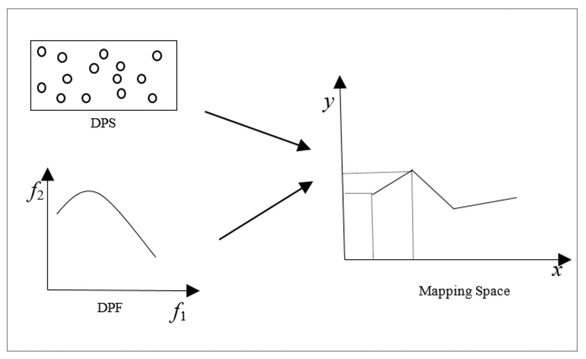
2.1. Problem Formulation

There are many formulations for dynamic multi-objective optimization problems. Without loss of generality, we considered a minimum DMOP in this study [18]:
min F x , t = f 1 x , t , f 2 x , t , , f M x , t T s . t . x Ω = i = 1 n [ a i , b i ]
where x = (x1, x2, x3, …, xn)T is an n-dimensional decision vector, and Ω is the decision space. F(x, t): Rn × TRM denotes an M-dimensional objective space, which contains M objectives that have some environmental changes during the evolutionary process. What’s more, we suppose that all the objective functions are continuous. There are three definitions of dynamic Pareto as follows.
Definition 1.
(Dynamic Pareto Dominance [19]): In a dynamic environment, a decision vector x1 Pareto dominates another decision vector x2 at the time windowt, expressed asx1x2, if and only if
i = 1 , , M , f i ( x 1 , t ) f i ( x 2 , t ) i = 1 , , M , f i ( x 1 , t ) < f i ( x 2 , t )
Definition 2.
(Dynamic Pareto-optimal Set (DPS) [12]): For a fixed time window t and a decision vectorx*∈ Ω, when there is no other decision vectorx∈ Ω such thatxdominatesx*, the decision vectorx*is said to be nondominated. The dynamic Pareto-optimal set (DPS) is the set of all non-dominated solutions in decision space, which can be represented by:
D P S ( t ) = { x * Ω | x Ω , x x * }
Definition 3.
(Dynamic Pareto-optimal Front (DPF) [12]): Similar to the static Pareto-front, the dynamic Pareto-optimal front (DPF) is the set of the corresponding objective values of the DPS:
D P F ( t ) = { F ( x * , t ) | x * D P S }
Based on the above definitions, the following statement can be made. Since an environmental change can lead to changes of DPS or DPF, an effective dynamic multi-objective optimization evolutionary algorithm (DMOEA) is expected to track the moving DPF in time and still maintain diversity and convergence.

2.2. Evolutionary Algorithms for DMOPs

Due to their wide application in real-world problems, they have acquired rapidly increasing attention in recent years. Because of the changes of DPS and DPF, DMOEAs pose a higher requirement of efficiency compared with static MOEAs. A well-designed DMOEA should perform well in maintaining both convergence and diversity of the population. Many improved classic evolutionary algorithms can be used in the process of solving DMOPs, such as multi-objective evolutionary algorithm based on decomposition and a first-order difference model (MOEA/D-FD) [20], the dynamic non-dominated sorting genetic algorithm (DNSGA-II) [21], a novel dynamic multi-objective evolutionary algorithm with a cell-based rank and density calculation strategy (DMOEA) [22], and dynamic constrained optimization differential evolution (DyCODE) [23].
As mentioned in Section 1, memory and prediction techniques are general methods for DMOPs and various studies have proposed prediction-based approaches. From the perspective of evolutionary process, prediction-based methods, can generally be divided into two classes: (1) population-based prediction and (2) individual-based prediction. In population-based prediction, the whole population is optimized with a single prediction model while the moving location of each individual is predicted in individual-based prediction methods. Teodoro et al. [24] proposed a method of plane separation for a whole population to solve DMOPs with incorporated references. In terms of computational cost, many algorithms focus on distribution but ignore the excessive computational burden. Moreover, a knee-guided prediction evolutionary algorithm (KPEA) [25] has been proposed to achieve a lower computational cost. Specifically, KPEA generates the non-dominated solutions around the knee points and boundary regions, and then relocates the location of the knee point and boundary regions. Zhou et al. [26] introduced two strategies for application in the process of population re-initialization. The two strategies are based on individuals in the population, and some individuals are predicted according to the information obtained from past environments. A feed-forward prediction approach, which combines a forecasting technique to place an anticipatory group of individuals, was introduced by Hatzakis et al. [27]. Taking the relevance between previous environments and new environment into account, Liu et al. [28] stored the solutions in the past environments into two different archives, so that the stored solutions will provide the information to find the optimal solutions when the next change occurs. Many DMOPs in real-world applications have various characteristics, such as the interval characteristic, which is one of the common applications in DMOPs. To solve interval DMOPs (DI-MOPs), Gong et al. [29] proposed a novel co-evolutionary model in terms of interval similarity. The interval parameters are set, and two different response strategies for change are applied to track the DPF. Wang et al. [30] presented a predictive method based on a grey prediction model, which divided the population into some clusters, then the centroid of each cluster was used to build the model. In addition, individuals from different clusters were selected to detect the environmental change.
Herein, we used various standards to measure the performance of a DMOEA in the evolutionary process, which is largely influenced by the speed of convergence and diversity. DMOEAs with rapid convergence track the moving DPF rapidly, while DMOEAs with good diversity pursue the effective distribution of the optimal solutions. Keeping a good balance between population diversity and convergence is critical to the performance of DMOEAs. For DMOPs, Chang et al. [31] combined query-based learning with particle swarm optimization (QBLDPSO) to improve the diversity of a population. Instead of maintaining the diversity of particles passively like typical PSO, QBLDPSO actively employs quantum parameter adaptation to achieve population diversity. In order to accelerate the convergence, Liang et al. [32] classified the decision variables into different groups according to different optimization stages, like change detection stage, optimization stage in each time window. The different crossover operators are employed to keep a balance of convergence and diversity.
There are many application scenarios for dynamic optimization algorithms. For example, Wang et al. [33] improved PSO with a mixed-integer programming model and four match-up strategies to manage dynamic scheduling problems with random job arrivals. Luna et al. [34] presented a novel restart method that can react to the changes in the traffic demands, improving the energy efficiency in the fifth generation (5G) of cellular networks. A novel chance-constrained dynamic optimization method, proposed by Zhou et al. [35], was applied to solve real industrial process issues. In the study of humanoid robots, losing balance and falling down are common problems. Chang et al. [36] applied a DMOEA to the falling down process of robots and was able to reduce damage to the robots. A dynamic multi-objective approach can also be applied to heterogeneous systems. For instance, [37] introduced a multi-objective dynamic load balancing (DLB) approach combined with a genetic heuristic engine, to enhance performance and code portability for such systems.
From the review above, we can identify three essential parts that should be included in an ideal DMOEA, which are change detection, change reaction, and multi-objective optimization. Herein, Algorithm 1 was prepared as the major frame of DMOEA. In the algorithm, after initializing the current generation, some strategies are used for change response when an environmental change occurs. The initialized population will be updated with these useful strategies, and the time window T is going to increase by one, which means the next environmental change. In the next step, the i-th multi-objective problems are optimized using a multi-objective evolutionary algorithm (MOEA) for one generation. The static MOEA employs the updated population as the initial population. At last, if the stop condition is not met, the process is repeated, otherwise the optimization of the next generation will be conducted.
Algorithm 1 The main frame of DMOEA
Input: the number of generations, g;
    the time window, T;
Output: optimal solution x* at every time step;
 1:  Initialize population POP0;
 2:  while stop criterion is not met do
 3:   if change is detected then
 4:    Update the population using some strategies: reuse memory, tune parame-ters, or predict solutions;
 5:    T = T + 1;
 6:   end if
 7:   Optimize T-th population with an MOEA for one generation and get optimal solution x*;
 8:  end while
 9:  g = g+1;
10:  return x*.

3. NSGA-III and Proposed Strategies

3.1. NSGA-III

There are many classical algorithms for multi-objective or many-objective problems. NSGA-III [17] is one of the classical multi-objective evolutionary algorithms (MOEAs) for static many-objective problems. NSGA-III adds the idea of reference points as an enhancement of NSGA-II [2], which is mainly used for dealing with multi-objective problems. The major framework of NSGA-III is similar to the original NSGA-II algorithm, except for the differences between their environmental selection in the critical layer. The NSGA-II method applies congestion and comparison operation to select and maintain diversity. Comparatively, NSGA-III employs well-distributed reference points to maintain the diversity of a population. Most MOEAs are more effective in solving problems with fewer objectives. When the number of objectives is greater than or equal to four, many methods have reduced selection pressure due to increased dimensions, and the effect is not ideal. Different non-dominated fronts are classified using the method of fast non-dominated sorting. In the selection stage, the congestion distance method is changed to the reference points method, because the former does not perform well for balancing the diversity and convergence in NSGA-II. It is also limited to solving various unconstrained problems, such as normalization, scaling, convexity, concavity, and convergence to the PF plane. In addition, the dynamic version of NSGA-II has been proposed for DMOPs, which was used for comparison in our experiments and NSGA-III was chosen as the evolutionary algorithm combined with the two proposed strategies.
The whole detailed process of NSGA-III is given in Algorithm 2. Firstly, reference points are defined and the initial population is obtained through generating a set of uniformly distributed points randomly. Secondly, genetic operators are used to generate the offspring, and then non-dominated sorting is conducted. The parent population Pt and the generated offspring Qt are combined as a new population Rt. The new population is placed in a non-dominant order, which means that the solutions in Rt are divided into different non-dominant levels. The N individuals that make up the next population will be selected from the mixed population. If the individuals in the first l − 1 non-dominated layer are exactly equal to N, then these individuals directly form the next generation population Pt+1. Otherwise, the remaining solutions of Pt+1 are selected from Fl according to the selection mechanism. Then, normalizing the objectives and each solution will be associated with one reference point. The closest K individuals associated with the reference points are selected. Finally, the best N solutions in the combined population are selected, and the next population Pt+1 is obtained.
Algorithm 2 The procedure of NSGA-III
Input: parent population, Pt;
   the archive population, St;
   i-th non-dominated front, Fi;
Output: the next population, Pt+1;
 1:  Define a set of reference points z*;
 2:  Generate offspring Qt through cross and mutation using GA operator;
 3:  Non-dominated sorting (Rt = PtQt);
 4:  while |St| < N do
 5:   St = StFi;
 6:   i = i + 1;
 7:  end while
 8:  Fl = Fi;
 9:  if |St| = N then
10:    Pt+1 = St;
11:  else
12:    Pt+1 = F1F2 ∪ … ∪ Fl−1;
13:  end if
14:  Normalize objectives and associate each solution with one reference point;
15:  Calculate the number of the associated solutions;
16:  Choose K = N − |Pt+1| solutions one by one from Fl;
17:  return Pt+1.

3.2. Change Detection

As mentioned above, one of the critical steps for DMOPs is change detection. Before using the change response strategy, change detection is necessary for dynamic multi-objective evolutionary algorithms (DMOEAs). The main process of environmental change detection is described in Algorithm 3, wherein we define a label flag indicating whether a change occurs. The initial value of flag is set to zero when the change detection starts. Then, individuals randomly selected from the initial population are evaluated for change detection. Herein, 20% of randomly selected individuals are used in our proposed algorithm, and their objectives are stored into Ps, which are then re-evaluated. By investigating whether there is a difference in the objective values between two generations, the results about whether a change occurs can be shown obviously. If there is a difference between the two generations, the value of a flag is set to one, and it can be said that an environmental change occurs and the change detection process ends.
Algorithm 3 Change detection
Input: the initial population, PT;
   the current number of iterations, g;
   the number of objective functions, F;
   the individual in population, p;
   stored individuals from past environment, Ps;
   the current time window, t;
Output: the sign indicating whether a change occurs, flag;
 1:  flag = 0;
 2:  Select randomly individuals from population PT, and store individuals into Ps;
 3:  for every pPs, iF do
 4:   Caculate fi(p, t);
 5:   fi(Ps) = fi(p, t);
 6:  end for
 7:  g = g + 1;
 8:  for every pPs do
 9:   Caculate fi(p, t);
10:   if fi(p, t) ≠ fi(Ps) then
11:    flag = 1;
12:    t = t + 1;
13:    break;
14:   end if
15:  end for
16:  return flag.

3.3. Second-Order Difference and Random Strategies

We propose a new strategy named the second-order difference strategy for DMOPs in this paper. This strategy is based on the first-order difference strategy, which used the centroid of the decision space to describe the trajectory of moving solutions over time. Let CT be the centroid of the DPS and PT be the obtained DPS at the time window T, then CT can be calculated by the following formula:
C T = 1 P T x P T x
where CT+1 represents the center of the decision space at the next time window, T + 1, which can be obtained by Formula (6):
C T + 1 = C T + C T C T 1
where |PT| is the cardinality of PT; and x is a solution of decision space in PT. The initial individuals of the population are provided through the prediction model at each generation. As we can see, the first-order difference model employs the centroid of the decision space, and predicts the next centroid for the next time window. Under the dynamic environment, objective functions change over time, but there is a certain relationship between the two objectives before and after the change.
Therefore, we can predict the next solution distribution using the information about the optimal solution before the change. In our proposed second-order difference strategy, the centroid of the objective space is also taken into account. The difference from the first-order difference model is that we consider both objective values and solutions in the decision space. The solutions in DPS and the corresponding objectives in DPF are mapped to a new two-dimensional mapping space (MS). The x-coordinate of this new plane is the set of DPS, and the y-coordinate is the average of objective values. Our proposed strategy is built-in two-dimensional space, and the centroid is the center of the two-dimensional plane related to the objectives. The mapping relation of the strategy is as Figure 1. Therefore, we can define a new CT, which can be computed by:
C T = 1 max ( P S T , P F T ) i = 0 i = P S T E u c l i d e a n [ ( x i , y i ) , ( x i + 1 , y i + 1 ) ]
where nt and |PFT| are the cardinality of DPS and DPF, respectively; (xi, yi) represents the vector in two-dimensional space, consisting of the optimal solution and the corresponding objective function value; and Euclidean() means to obtain the Euclidean distance between two points in the plane. Similar to the first-order difference model, the location of the centroid at the next time window T + 1 is predicted using the formulation as follows:
C T + 1 = C T + C T C T 1
After determining the centroid location of the next time window, random strategy is then applied to the Algorithm 1 presented in this paper. The random strategy is the random perturbation around the obtained centroid position, so as to obtain a series of solutions similar to the last change. The radius of random strategy is set to 0.1, which means that we will take uniformly random points on the plane centered at the centroid and with the radius. The performance of this strategy can be shown through our next comparative experiments. The whole process of our proposed strategy combined with NSGA-III is described in Algorithm 4.
Some similarities and differences exist between our proposed strategy and the first-order difference model, where the former strategy is based on the latter. Both strategies use Formula (8) to obtain the next centroid, this is why they are called “difference strategies”, and the difference between them is the way the centroid is generated. Obviously, the first-order difference strategy employs the simplest method to generate the centroid by only considering the center of DPS. However, when facing environmental changes, the objectives will change in a big or small way and, therefore, should be considered when looking for the centroid. In this way, the objective space can have a certain relationship with the last change, so as to predict more accurate solutions. Our algorithm is proposed based on this background, and the details of the algorithm are given in Algorithm 4.
At the beginning of the evolutionary process, the individuals of the population are initialized randomly, and the initial population is reevaluated. Then the change detection process described in Algorithm 3 is conducted. When an environmental change occurs, the population must be updated to respond to the change. As mentioned in Algorithm 4, the new population is composed of three kinds of individuals: the old solutions, the prediction solutions obtained by our proposed strategy and the random solutions around the prediction solutions. In most cases of real-world DMOPs, there are some similarities between the DPS of the consecutive DMOPs. Therefore, a certain percentage of old solutions can be reserved for the next population at the new time window. The old solutions from the last environment may perform better than reinitialized solutions. Besides, our prediction solutions and the old solutions are put into the new population uniformly, and the predicted centroid in the new environment can be described according to (7). Some random solutions around the predicted centroid are introduced as well, which adds diversity to the new population.
Algorithm 4 Second-order random strategy combined with NSGA-III
Input: the current population, PT;
   the time window, T;
   the number of individuals in population, N;
   the historic centroid points, CT−1;
   the centroid of time window T, CT;
Output: the next population PT+1;
 1:  Initialize population PT and evaluate the inital population PT;
 2:  Change detection (PT);
 3:  if change is detected then
 4:   while the maximum number of iterations is not reached do
 5:    for i = 1:N do
 6:     if mod(i, 3) == 0 then
 7:       x i T + 1 = x i T + C T C T 1 ;
 8:      Random perturbation around x i T + 1 ;
 9:     else
10:       x i T + 1 = x i T ;
11:     end if
12:     Use NSGA-III to optimize x i T + 1 and get the next generation population PT+1;
13:    end for
14:   end while
15:  end if
16:  T = T + 1;
17:  return PT+1.

4. Experiments

All the experiments were conducted on MATLAB R2018a. Intel(R) Core (TM) i3-8100 CPU @ 3.60GHz was used as the hardware environment.

4.1. Benchmark Problems and Performance Metrics

In order to study the performance of our proposed strategies, two parts of the experiments were conducted for DMOPs. In this paper, six benchmarks with different change types were used for confirmation. The instances and definitions are listed in Table 1, and the functions have two objectives. The common formula of a bi-objective dynamic benchmark, which adds the time window parameter in forming the static ZDT [38] problems, can be described as follows:
min f ( x , t ) = ( f 1 ( x I , t ) , g ( x I I , t ) h ( x I I I , f 1 ( x I , t ) , g ( x I I , t ) , t ) )
where xI, xII, and xIII are three different subsets of design variables set x in decision space. For Fun1, as the environment changes, the DPS of Fun1 changes, whereas the moving DPF of Fun1 remains unchanged. In addition, the DPF of Fun1 is convex. Some parameters that do not require introduction include τ, which is the generation counter, and nt, which represents the number of distinct steps in a fixed t. τT and nt are two parameters that reflect the frequency and severity of an environmental change, respectively. In the benchmarks definitions, the time instance t can be computed by t = (1/nt) ∗ (τ/τT). Different from Fun1, both DPS and DPF of Fun2 change over time, and DPF change from convex to nonconvex. The convergence speed and reactivity when the environment changes can be evaluated by Fun3 and Fun5 benchmarks. Specifically, the time-varying nonmonotonic dependencies between any two decision variables are introduced in Fun3, which is similar to the greenhouse system in the real world. As the time window increases, the dependency between two variables becomes more complicated, and the density of solutions also changes over time. Therefore, the relation between the decision variables and the diversity performance can also be assessed by Fun3 for DMOPs. Fun5 is a dynamic function with dynamic DPFs and DPSs, and the overall objective vectors change between several modes as the DPS changes. Fun5 is similar to the electric power supply system [39] in real-world applications. The DPF of Fun4 has a general change trend, which changes from convex to concave, and the values in both the DPF and DPS differ under different time windows. For Fun6, the characteristics of the DPS and DPF are totally different. The DPS is simpler than the DPF of Fun6, which specifically contains some locally linear, concave, or convex segments. What’s more, the number of local segments is unfixed. The main characteristics of the six benchmarks mentioned above are summarized in Table 2.
Based on the benchmarks above, we tested our proposed algorithm under two different dynamic parameters. We set the change severity, nt, to 5 and 10, and set the change frequency τT to 5, 10, and 20 respectively, which represents severe, moderate, and slight environmental changes. Therefore, we obtained six different sets of parameter values, namely (5, 5), (5, 10), (5, 20), (10, 5), (10, 10), and (10, 20). Each benchmark has six different cases with different parameters, and therefore, there are total of 36 cases in the six benchmarks. Then, six benchmark problems with different parameters were conducted, and three different dynamic metrics were employed to evaluate the performance of SDNSGA-III.
As we know, there are various performance metrics to assess the algorithm, such as inverted generational distance (IGD), generational distance (GD), and hypervolume (HV). For dynamic environment, a modified version of the IGD, HV, and GD is employed to evaluate the performance of DMOEAs. The MIGD metric proposed by Zhou et al. [43] is the dynamic version of IGD, which introduces the time window parameter, whereby the basic definition of MIGD metric is the average of IGD over a period of time. The definition of IGD can be described as follows. Let S be the solution set obtained by the algorithm, and P* be a set of reference points that is uniformly sampled from DPF. Therefore, we can calculate IGD as:
I G D ( S , P * ) = x P * min y S d i s ( x , y ) P *
where dis(x, y) means the Euclidean distance from x in reference set P* to y in solution set S. Both the convergence and diversity of an algorithm can be assessed by computing IGD at the same time. In addition, the smaller the IGD value is, the better the comprehensive performance of an algorithm. This is similar to a MIGD metric. The MIGD metric we used to evaluate DMOEAs can be formulated as:
M I G D = 1 T t T I G D ( S , P * )
The HV is also one of the frequently used evaluation metrics, which represents the volume of the region that is rounded by the non-dominated solution set obtained by the algorithm and the reference points. HV can be described as:
H V ( S * , v i ) = δ ( i = 1 S * v i )
where δ is a Lebesgue measure to caculate volume; |S*| is the number of non-dominated solutions sets; and vi represents the super volume composed of the reference points and the i-th solution in the solution set. The MHV [44] metric is a modified dynamic version of the static HV metric, which is formulated as:
M H V = 1 T t T H V ( S * , v i )
The metric GD measures the diversity of an algorithm and describes the average of the minimum Euclidean distance from each point in the solution set S to the reference set P*. Under dynamic environments, the MGD metric is proposed to measure the performance of an algorithm instead of GD. Similar to MIGD and MHV, MGD is the modified version of GD, which can be defined as:
G D ( S , P * ) = y S min x P * d i s ( x , y ) 2 P
M G D = 1 T t T G D ( S , P * )
In our experiments, we used MIGD, MHV, and MGD metrics to measure the performance of our proposed SDNSGA-III algorithm. T refers to a set of discrete time instances in a single run. Further, |T| is the cardinality of T in the definitions of MIGD, MHV, and MGD. Our experiments were mainly conducted to measure the performance of NSGA-III combined with our proposed strategies. The experiments were divided into two parts: (1) the to compare the results of SDNSGA-III and the other four popular algorithms, and (2) to compare NSGA-III with different strategies to prove the effectiveness of the second-order difference strategy and random strategy. The general parameters in all algorithms are presented in Table 3.

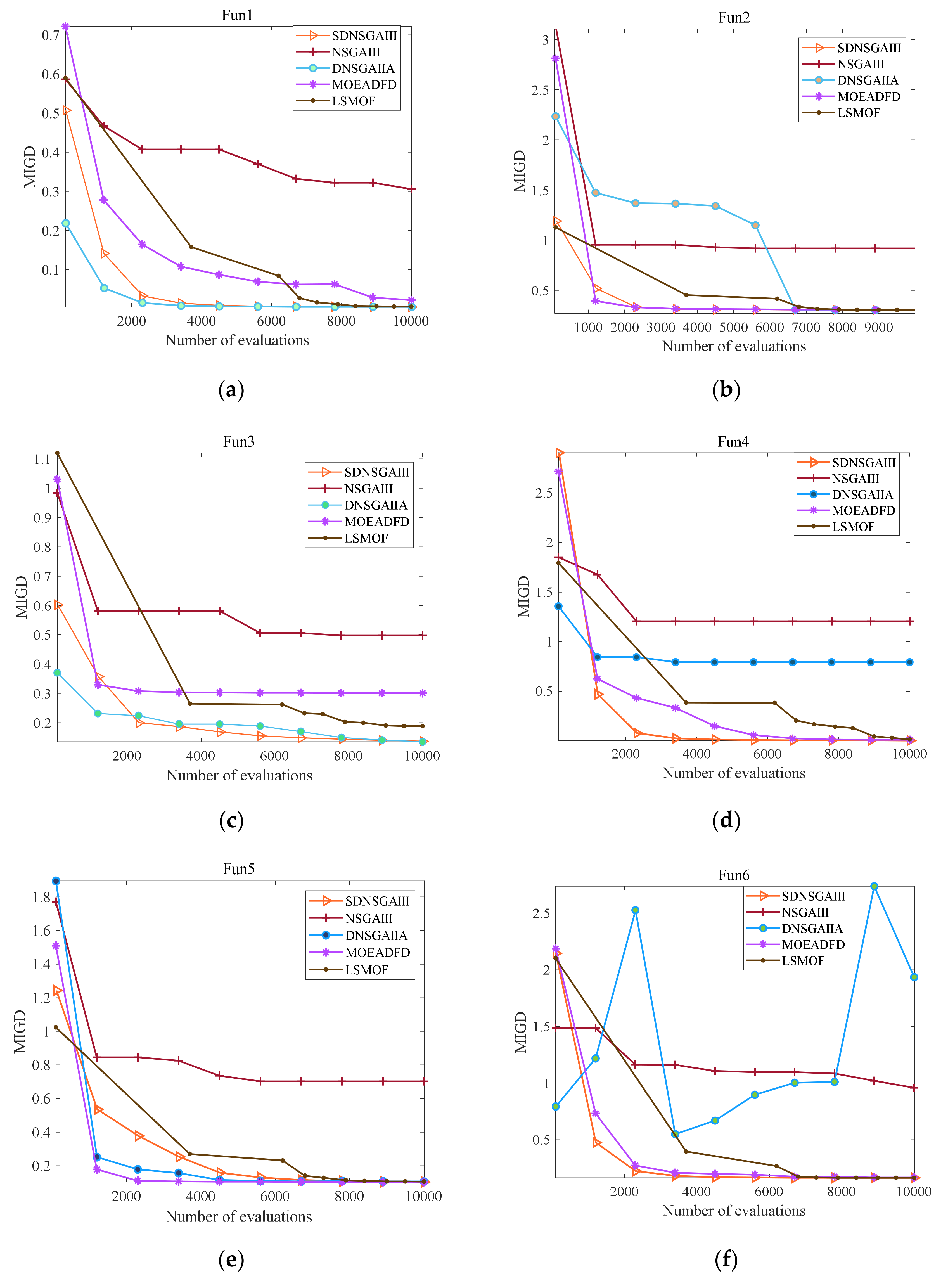
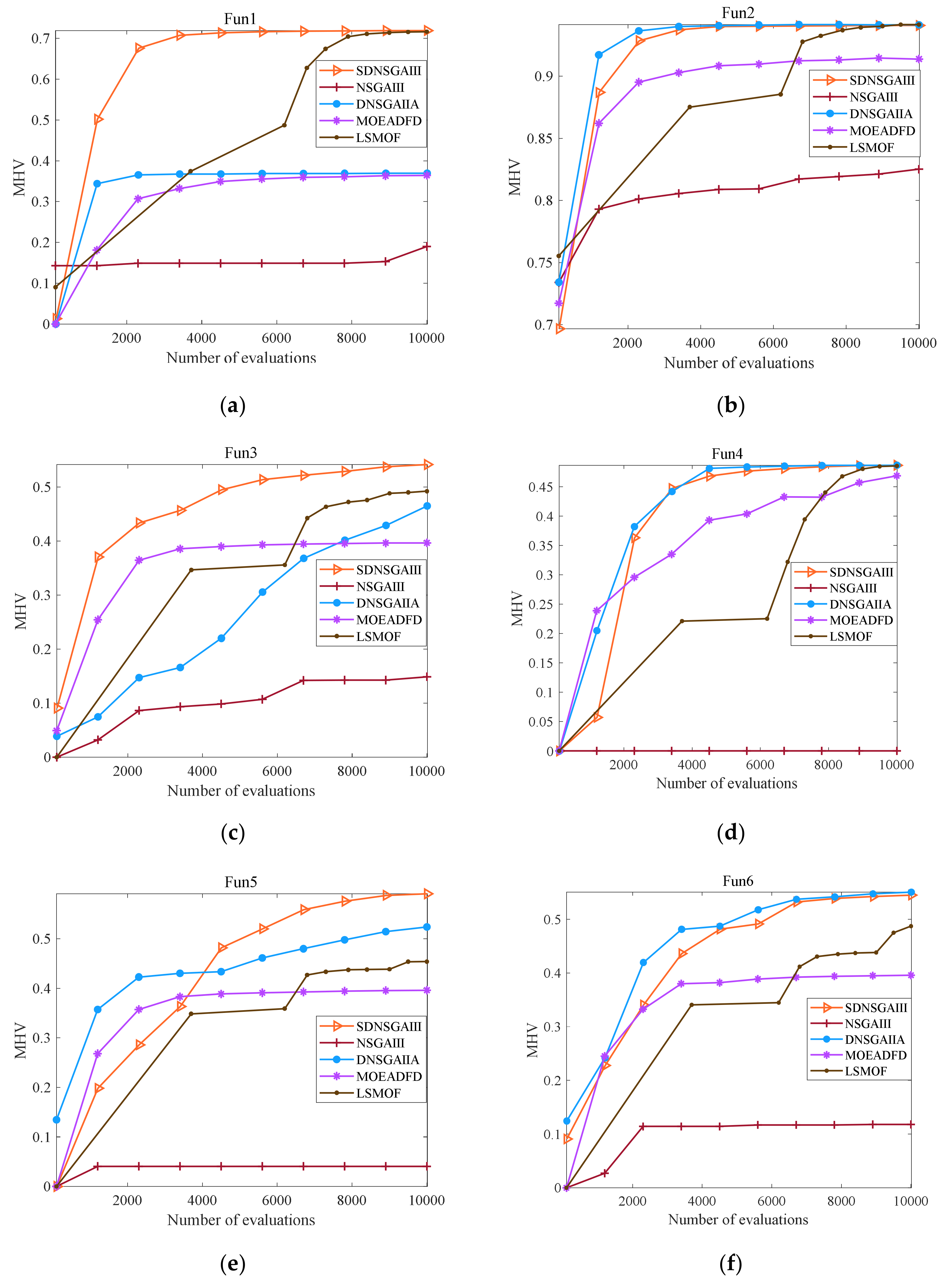
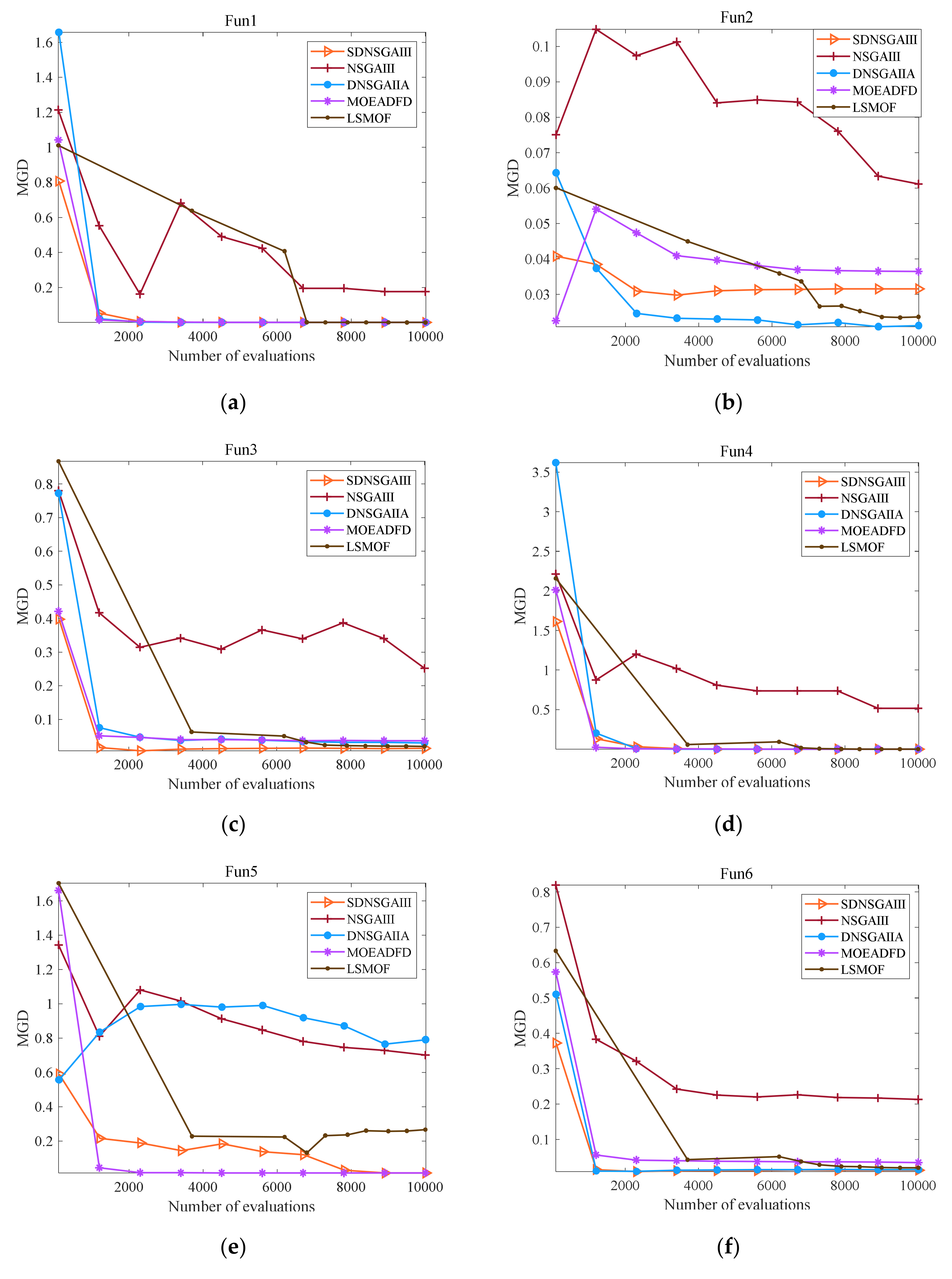
4.2. Comparative Study for the Proposed Algorithm

Our proposed algorithm (SDNSGA-III) was compared with four state-of-the-art algorithms, including NSGA-III [17], DNSGA-II-A [21], MOEA/D-FD [20], and a multi-objective optimization framework (LSMOF) [45]. The comparison between SDNSGA-III and NSGA-III was made to prove the performance of our proposed strategies. Based on the differences in the performance metrics, we can determine the results of whether our second-order strategy and random strategy can obtain better convergence and diversity. DNSGA-II-A [21] and MOEA/D-FD [20] are DMOEAs that are primarily deal with dynamic problems. Particularly, DNSGA-II-A [21] introduces some new random individuals when a new population is generated. When merging the parent and child population into the next bigger population, all individuals are re-evaluated through the benchmarks. MOEA/D-FD [20] is a modified version of the original MOEA/D, which uses the first-order difference model. LSMOF reformulates the problems, tracks the Pareto optimal set directly, and also accelerates the computational efficiency of the multi-objective evolutionary algorithm.
The data in Table A1 (the first table in Appendix A) show the obtained MGD values and standard deviations over 30 runs. The last column in Table A1 means the percentage difference between SDNSGA-III and other four comparative algorithms. The positive (negative) value shows the performance of SDNSGA-III is better (worse) than the comparing algorithm. The performance evaluation was conducted at the 5% significance level. In Table A1, the results are recorded as “+”, “−”, and “=” for when SDNSGA-III performs significantly better than, worse than, and equivalent to the corresponding algorithm respectively. The bold font indicates that the algorithm has the best diversity on this benchmark. From Table A1, it is obvious that SDNSGA-III performed better than the other four algorithms in most cases, which means it has a better tracking ability of DPS and DPF. Moreover, the SDNSGA-III values in Table A1 are significantly better than those of NSGA-III, sufficiently proving that the second-order and random strategies improve the performance of NSGA-III for dealing with dynamic problems. Besides, from the perspective of different problems, SDNSGA-III performed best in Fun1, Fun4 and Fun6, while the performance of SDNSGA-III was roughly the same on Fun2 and Fun3. This means that our proposed strategy is more suitable for dynamic problems whose DPS changes. Although the performance on other problems was worse than on Fun1, Fun4 and Fun6, about 90% of the results are best among the five comparative algorithms. In general, our proposed strategy worked well for different DMOPs. What’s more, when change severity was relatively smooth (nt = 10), the five sixth values of SDNSGA-III were better than the other four algorithms. In addition, when the change frequency was fast (τT = 5), all results of the other comparative algorithms were worse than those of SDNSGA-III. Therefore, it can be suggested that our proposed strategy can obtain the best diversity performance of the population when the change is smooth and fast. The reason for this result is that when the change frequency is fast, our proposed strategies enhance the search efficiency and accuracy of tracking the moving DPF.
In order to investigate the convergence process of the algorithms, the MIGD, MHV, and MGD trends of Fun1–6 with a fixed nt and τT were investigated, as shown in Figure 2, Figure 3 and Figure 4. In Figure 2a–f, the overall trend was obviously downward. A total of 10 points were sampled randomly within a single run, and the evaluation numbers was set to 10,000. As the evaluations increased, the metrics of all five algorithms tend to become relatively stable. Among the compared algorithms, generally speaking, SDNSGA-III reached a better MIGD value in less time, as observed in Figure 2a–d,f. For Fun1 and Fun2, DNSGAII-A and MOEAD-FD obtained a lower MIGD at the beginning of the evaluations, and our proposed SDNSGA-III reached almost the same value in the later stage of evaluations. In Figure 3, contrary to MIGD, the general tendency of MHV exhibited an increase, while the MHV value of SDNSGA-III was higher than the other comparative algorithms observably on Fun1, Fun3, and Fun5. SDNSGA-III reached almost the same MHV as MOEAD-FD at the end of evaluations in Figure 3b,d,f, which means SDNSGA-III has a similar tracking ability with MOEAD-FD on Fun2, Fun4, and Fun6. The overall trend of MGD in Figure 4 is similar to MIGD, and SDNSGA-III performed more stable than the other comparative algorithms. Figure 2, Figure 3 and Figure 4 further reveal that our proposed SDNSGA-III has a great improvement in tracking DPF and DPS compared with NSGA-III, and SDNSGA-III performed more stable than other algorithms with a steady tracking ability regardless of the environmental change.
The statistical results of six benchmarks and six parameters on MIGD, MHV, and MGD are recorded in Table 4 and Table 5 respectively. Among the six different benchmarks, SDNSGA-III reached 18 best results on Fun1, which has dynamic DPS and static DPF. In terms of the six different parameters, our proposed SDNSGA-III achieved the best metric values on the severe change severity (nt = 5) and the slow change frequency (τT = 20). The performance of SDNSGA-III was nearly the same on the rest of the five parameters. Generally, SDNSGA-III is more suitable for DMOPs, since it has a relatively smooth change or fixed DPF. This can be attributed to the prediction strategy that can achieve a centroid location more accurately with a slight change, while the prediction error increases with a severe and fast change. Even so, SDNSGA-III performed better than the other comparative algorithms on most test instances. To further evaluate the performances of the second-order strategy and random strategy, the comparisons between the two are discussed in the next section.

4.3. Comparative Study for Two Proposed Strategies

In the comparative study, the performances of the second-order difference strategy and random strategy were analyzed. NSGA-IIIs is the algorithm with the second-order difference strategy without random strategy, while NSGA-IIIr incorporates the random strategy without the second-order difference strategy. The main process of NSGA-IIIr is to first initialize the population, then use NSGA-III to optimize individuals at each generation. When a change is detected, random perturbation is conducted around the optimal solution of the previous generation. The comparative results show the efficiency of the second-order difference strategy and random strategy in SDNSGA-III.
Table A2 (the second table in Appendix A) depicts the MIGD values and standard deviations obtained by the four algorithms over 30 runs. In the table, about 67% of the results clearly reveal that the performance of SDNSGA-III is better than the other three comparative algorithms. In general, both NSGA-IIIs and NSGA-IIIr algorithms demonstrated little difference in performance. However, it is obvious that SDNSGA-III, which combines both strategies, performed best among all four algorithms. Besides, NSGA-IIIr performed mostly better than NSGA-IIIs in Fun3 and Fun6. In other words, the random strategy improves the diversity of SDNSGA-III in a dynamic environment. Furthermore, NSGA-IIIs exhibited better values than NSGA-IIIr with a smooth change severity and fast change frequency. This proves that our proposed second-order difference strategy could track the moving DPS and DPF directly, and the random strategy can improve the diversity ability of NSGA-III on DMOPs. Since random strategy can better adapt to dynamic characteristics for DMOPs, the SDNSGA-III algorithm exhibited the best comprehensive performance among all comparative algorithms.
Table 6 and Table 7 include the statistical results from different perspectives, including the different benchmarks and parameters. In the tables, “a/b/c” represents the number of best MIGD, MHV, and MGD metric values, respectively. In Table 6, the data obviously show that SDNSGA-III combined with the two strategies performed best, and a single NSGA-III performed worst among the four comparative algorithms. NSGA-IIIs showed an obviously better performance than NSGAIIIr on Fun2 and Fun4. For the benchmarks of Fun3 and Fun6, NSGA-IIIr performed better than NSGA-IIIs, and both of algorithms performed the same on Fun1 and Fun5. These results demonstrate that SDNSGA-III effectively incorporates second-order difference strategy and random strategy to achieve the best metric values. It is pertinent to note that the former strategy is more applicable to DMOPs whose DPS and DPF changes from convex like Fun2 and Fun4. When dealing with more complex DMOPs, like Fun3 and Fun6, whose DPS and DPF change irregularly, the latter strategy behaves better. Table 7 represents the statistical results of the different change frequencies and change severities. When the change severity nt was fixed to 10 and the change frequency τT was set to 20, SDNSGA-III reached the best metric values. In addition, the performance of SDNSGA-III with higher change severity and higher change frequency was better than the other comparative algorithms. When nt and τT change, the random strategy can ensure the diversity in a population, while a single second-order strategy cannot track the moving DPF accurately. The statistical data in Table 6 and Table 7 illustrate that combining the second-order difference strategy and random strategy is indeed effective to solve DMOPs better.

5. Conclusions

In this study, we propose a novel algorithm based on NSGA-III, which incorporates a second-order difference strategy and random strategy to solve DMOPs. These two strategies are specifically employed to predict the next centroid location based on its historical locations and random disturbances around the predicted centroid location when change is detected. Moreover, the performance of SDNSGA-III was validated using different benchmarks and different metrics via testing on different change frequencies and change severities. Compared with four other state-of-the-art evolutionary algorithms, our SDNSGA-III can obtain a better convergence speed and maintain diversity of a population when tracking the moving DPS and DPF. In addition, a comparison between the two proposed strategies was conducted to verify their effectiveness. It was found that the second-order difference strategy and random strategy have the ability to find the moving DPF, and SDNSGA-III can maintain the diversity of a population to respond to environmental change. In addition, the further innovations about prediction can be inspired through the proposed second difference strategy.
Despite our promising findings, some issues need to be further addressed. For example, more benchmarks should be employed to evaluate the performance of SDNSGA-III. Moreover, further studies are suggested for other state-of-the-art algorithms incorporated with second-order difference and random strategies to show their ability to enhance searching efficiency. The second-order difference strategy can be incorporated with other effective frameworks to increase the accuracy of prediction at the stage of change response. What’s more, we tested our strategies only on two-objective benchmarks in this work. Therefore, we plan to focus on more than two-objective dynamic optimization problems in future studies.

Author Contributions

H.Z.: Conceptualization, methodology, software, visualization, investigation, writing—original draft preparation; G.-G.W.: supervision, validation, data curation, reviewing and editing; J.D.: visualization, reviewing and editing; A.H.G.: project administration, reviewing and editing. All authors have read and agreed to the published version of the manuscript.

Funding

This research was funded by National Natural Science Foundation of China, Grant Numbers U1706218, 41576011, 41706010, and 61503165.

Institutional Review Board Statement

Not applicable.

Informed Consent Statement

Not applicable.

Data Availability Statement

Not applicable.

Conflicts of Interest

The authors declare no conflict of interest.

Appendix A

Table A1. The MGD values and standard deviations obtained by five algorithms.
Problem(nt, τT)SDNSGA-IIINSGA-IIIDNSGA-II-AMOEA/D-FDLSMOFPercentage Difference
Fun1(5,5)9.7641e-5
(2.05e-5)
8.3088e−1
(2.10e−1) −
1.8830e−4
(2.55e−5) −
5.9543e−4
(1.26e−4) −
3.4402e−4
(8.51e−5) −
99.99%, 48.15%,
83.60%, 71.62%
(5,10)1.0885e−4
(2.53e−5)
2.5769e−1
(1.35e−1) −
1.9373e−4
(3.34e−5) −
6.2599e−4
(1.63e−4) −
3.3416e−4
(5.25e−5) −
99.96%, 43.81%,
82.61%, 67.43%
(5,20)7.2249e−5
(1.40e−5)
8.3223e−1
(2.49e−1) −
1.5780e−4
(2.44e−5) −
4.6507e−4
(9.94e−5) −
1.6833e−4
(3.98e−5) −
99.99%, 54.21%,
84.46%, 57.08%
(10,5)9.2895e−5
(2.21e−5)
1.6212e−1
(3.82e−2) −
1.8772e−4
(3.37e−5) −
6.2374e−4
(1.69e−4) −
2.9641e−4
(7.04e−5) −
99.94%, 50.51%,
85.11%, 68.66%
(10,10)9.4192e−5
(1.79e−5)
1.8184e−1
(5.75e−2) −
1.9987e−4
(3.70e−5) −
6.0922e−4
(1.70e−4) −
3.5548e−4
(9.81e−5) −
99.95%, 52.87%,
84.54%, 73.50%
(10,20)9.6531e−5
(1.98e−5)
2.7691e−1
(9.54e−2) −
1.9788e−4
(3.50e−5) −
6.2510e−4
(1.48e−4) −
3.2505e−4
(7.25e−5) −
99.97%, 51.22%,
84.56%, 70.30%
Fun2(5,5)1.5312e−2
(3.99e−5)
1.3209e+0
(3.64e−1) −
5.6395e−2
(7.95e−4) −
5.6148e−2
(2.25e−3) −
1.5518e−2
(2.13e−4) −
98.84%, 72.85%,
72.73%, 1.33%
(5,10)2.9755e−2
(4.91e−4)
1.1544e+0
(2.13e−1) −
4.9951e−2
(3.24e−4) +
5.4658e−2
(4.02e−3) −
3.0794e−2
(4.69e−4) −
97.42%, 40.43%,
45.56%, 3.37%
(5,20)1.2032e−4
(1.26e−4)
2.7577e−1
(7.57e−2) −
1.6799e−4
(7.21e−5) −
8.6767e−4
(7.26e−4) −
5.0816e−2
(1.39e−4) −
99.96%, 28.38%,
86.13%, 99.76%
(10,5) 5.1443e−2
(4.63e−6)
1.2241e+0
(3.38e−1) −
5.6449e−2
(5.87e−4) −
5.4444e−2
(2.26e−3) −
7.9690e−3
(1.07e−4) +
95.80%, 8.87%,
5.51%, −545.54%
(10,10)1.5329e−2
(8.66e−5)
2.2435e−1
(4.74e−2) −
1.5834e−2
(1.26e−4) −
1.6239e−2
(3.13e−4) −
1.6044e−2
(2.18e−4) −
93.17%, 3.19%,
5.60%, 4.46%
(10,20)2.9301e−2
(2.01e−5)
5.0671e−1
(1.11e−1) −
3.1420e−2
(3.74e−4) −
3.2043e−2
(5.79e−4) −
3.1609e−2
(3.73e−4) −
94.22%, 6.74%,
8.56%, 7.30%
Fun3(5,5)1.4966e−2
(7.01e−3)
2.2557e−1
(3.44e−2) −
1.5307e−2
(7.32e−3) −
3.8589e−2
(6.69e−4) −
2.1146e−2
(4.48e−3) −
93.37%, 2.23%,
61.22%, 29.23%
(5,10) 1.8975e−2
(3.09e−3)
2.2439e−1
(3.65e−2) −
1.8150e−2
(5.22e−4) =
4.0220e−2
(5.76e−4) −
2.2850e−2
(3.70e−3) −
91.54%, −4.55%
52.82%, 16.96%
(5,20)1.4379e−2
(3.98e−3)
2.2734e−1
(5.27e−2) −
4.0261e−2
(1.07e−3) −
3.4202e−2
(7.02e−3) −
2.0892e−2
(3.83e−3) −
93.68%, 64.29%,
57.96%, 31.17%
(10,5)1.4928e−2
(5.67e−3)
2.0592e−1
(4.43e−2) −
3.7969e−2
(5.04e−4) −
3.2770e−2
(5.84e−3) −
2.0691e−2
(3.76e−3) −
92.75%, 60.68%,
54.45%, 27.85%
(10,10)1.3473e−2
(6.74e−4)
2.1656e−1
(5.06e−2) −
1.6858e−2
(8.05e−3) −
3.2085e−2
(8.06e−3) −
2.8596e−2
(4.29e−3) −
93.78%, 20.08%,
58.01%, 52.89%
(10,20)1.4165e−2
(5.29e−4)
2.2959e−1
(6.38e−2) −
1.6997e−2
(8.25e−3) =
3.5214e−2
(5.84e−3) −
2.1800e−2
(1.92e−3) −
93.83%, 16.66%,
59.77%, 35.02%
Fun4(5,5)5.7478e−5
(3.03e−5)
3.0586e+0
(5.11e−1) −
1.2177e−4
(2.95e−5) −
5.9951e−4
(2.18e−4) −
1.2788e−4
(1.11e−4) −
100.00%, 52.80%,
90.41%, 55.05%
(5,10)9.8560e−6
(6.66e−6)
3.0143e+0
(5.17e−1) −
8.7865e−5
(3.11e−5) −
7.3340e−4
(2.66e−4) −
1.1863e−4
(3.68e−5) −
100.00%, 88.78%,
98.66%, 91.69%
(5,20)1.7514e−4
(3.61e−5)
1.1872e+0
(4.54e−1) −
2.0144e−4
(3.60e−5) −
1.3375e−3
(3.92e−4) −
3.3894e−4
(1.37e−4) −
99.99%, 13.06%,
86.91%, 48.33%
(10,5)8.6286e−6
(4.66e−6)
3.2288e+0
(7.88e−1) −
1.0346e−4
(3.86e−5) −
8.5105e−4
(4.65e−4) −
1.0690e−4
(3.37e−5) −
100.00%, 91.66%,
98.99%, 91.93%
(10,10)1.7192e−4
(3.61e−5)
8.0273e−1
(2.86e−1) −
1.9120e−4
(2.72e−5) −
1.2319e−3
(5.49e−4) −
3.0479e−4
(1.20e−4) −
99.98%, 10.08%,
86.04%, 43.59%
(10,20)1.5884e−4
(4.62e−5)
6.9277e−1
(2.27e−1) −
2.0395e−4
(2.67e−5) −
1.3210e−3
(3.97e−4) −
2.8649e−4
(8.88e−5) −
99.98%, 22.12%,
87.98%, 44.56%
Fun5(5,5) 2.2038e−1
(2.09e−1)
6.9385e−1
(1.30e−1) −
8.8662e−1
(2.03e−1) −
1.3465e−2
(5.94e−5) +
9.6630e−1
(1.22e−1) −
68.24%, 75.14%
−1536.69%, 77.19%
(5,10)1.3050e−2
(5.39e−5)
2.2280e−1
(5.30e−2) −
1.3435e−2
(2.36e−4) −
1.3153e−2
(2.04e−4) −
1.3589e−2
(1.58e−4) −
94.14%, 2.87%,
0.78%, 3.97%
(5,20) 1.2587e−2
(2.49e−5)
9.3152e−1
(1.74e−1) −
1.2475e−2
(2.03e−4) +
1.2611e−2
(2.55e−5) −
1.2590e−2
(2.18e−4) =
98.65%, −0.90%,
0.19%, 0.02%
(10,5)1.3049e−2
(4.49e−5)
2.0971e−1
(3.26e−2) −
1.3518e−2
(1.89e−4) −
1.3240e−2
(2.93e−4) −
1.3537e−2
(2.81e−4) −
93.78%, 3.47%,
1.44%, 3.60%
(10,10)8.0280e−3
(2.85e−6)
1.4576e+0
(2.94e−1) −
1.0723e+0
(1.56e−1) −
8.0422e−3
(1.63e−5) −
4.3435e−1
(2.46e−1) −
99.45%, 99.25%,
0.18%, 98.15%
(10,20)1.3176e−2
(1.01e−3)
8.7853e−1
(1.33e−1) −
7.4932e−1
(8.50e−2) −
1.3472e−2
(9.12e−5) =
4.1628e−1
(2.99e−1) −
98.50%, 98.24%,
2.20%, 96.83%
Fun6(5,5)1.4959e−2
(5.61e−3)
2.2469e−1
(5.33e−2) −
1.7703e−2
(8.50e−3) −
3.7265e−2
(6.28e−4) −
2.1705e−2
(2.33e−3) −
93.34%, 15.50%,
59.86%, 31.08%
(5,10)1.3725e−2
(5.89e−4)
2.1227e−1
(3.26e−2) −
1.8282e−2
(9.14e−3) −
3.7403e−2
(6.66e−4) −
2.1408e−2
(1.84e−3) −
93.53%, 24.93%,
63.31%, 35.89%
(5,20)1.3892e−2
(7.75e−4)
2.2927e−1
(7.10e−2) −
1.8479e−2
(8.87e−3) −
3.6830e−2
(3.22e−3) −
2.1563e−2
(2.41e−3) −
93.94%, 24.82%,
62.28%, 35.57%
(10,5)1.4122e−2
(1.49e−3)
2.1570e−1
(3.32e−2) −
1.5653e−2
(5.02e−3) −
3.5765e−2
(5.70e−3) −
2.2094e−2
(2.74e−3) −
93.45%, 9.78%,
60.51%, 36.08%
(10,10)1.4963e−2
(6.00e−3)
2.1200e−1
(3.18e−2) −
1.6425e−2
(6.86e−3) −
3.6488e−2
(4.24e−3) −
2.1332e−2
(2.62e−3) −
92.94%, 8.90%,
58.99%, 29.86%
(10,20)1.3778e−2
(6.56e−4)
2.1564e−1
(3.12e−2) −
1.6983e−2
(7.13e−3) −
3.6915e−2
(2.32e−3) −
2.1979e−2
(2.30e−3) −
93.61%, 18.87%,
62.68%, 7.31%
Table A2. The MIGD values and standard deviations obtained by four algorithms.
Problem(nt, τT)SDNSGA-IIINSGA-IIINSGA-IIIsNSGA-IIIrPercentage Difference
Fun1(5,5)4.1173e−3
(7.59e−5)
1.0619× 10+0
(3.04e−1) −
5.4190e−3
(7.05e−3) −
4.4643e−3
(2.05e−3) −
99.61%, 24.02%, 7.77%
(5,10)4.1621e−3
(1.09e−4)
3.1543e−1
(6.21e−2) −
4.1246e−3
(6.60e−5) +
4.7086e−3
(9.61e−4) −
98.68%, −0.91%, 11.61%
(5,20)4.0346e−3
(6.50e−5)
9.0279e−1
(2.77e−1) −
4.0621e−3
(1.80e−4) −
4.0917e−3
(2.52e−4) −
99.55%, 0.68%, 1.40%
(10,5)4.1143e−3
(1.10e−4)
3.1175e−1
(4.65e−2) −
4.1199e−3
(5.87e−5) −
4.1204e−3
(7.92e−5) −
98.68%, 0.14%, 0.15%
(10,10)4.1051e−3
(7.77e−5)
2.9676e−1
(4.29e−2) −
4.1788e−3
(2.68e−4) −
4.1059e−3
(6.46e−5) −
98.62%, 1.76%, 0.02%
(10,20)4.1219e−3
(8.22e−5)
3.2164e−1
(6.44e−2) −
4.1977e−3
(7.97e−5) −
4.1297e−3
(8.09e−5) −
98.72%, 1.81%, 0.19%
Fun2(5,5)5.2642e−1
(3.66e−6)
1.8119e+0
(4.16e−1) −
5.2047e−1
(4.95e−3) +
5.2795e−1
(5.98e−3) −
70.95%, −1.14%, 0.29%
(5,10)5.2642e−1
(7.13e−6)
1.5026e+0
(2.98e−1) −
3.0454e−1
(1.22e−3) +
3.0438e−1
(1.73e−3) +
64.97%, −72.86%,72.95%
(5,20)4.1727e−3
(1.60e−4)
6.5787e−1
(1.70e−1) −
5.2028e−1
(4.53e−3) −
5.2708e−1
(6.02e−3) −
99.37%, 99.20%, 99.21%
(10,5)5.2642e−1
(3.09e−6)
1.8949e+0
(2.94e−1) −
7.8633e−2
(1.47e−4) +
7.8664e−2
(1.37e−4) +
72.22%, −569.46%, −569.20%
(10,10)1.5659e−1
(1.74e−4)
5.1829e−1
(6.53e−2) −
1.5659e−1
(1.79e−4) =
1.5660e−1
(1.74e−4) −
69.79%, 0.00%, 0.01%
(10,20)3.0300e−1
(1.75e−4)
9.4884e−1
(1.59e−1) −
3.0392e−1
(1.08e−4) −
3.0397e−1
(1.69e−4) −
68.07%, 0.30%, 0.32%
Fun3(5,5)1.3632e−1
(7.43e−3)
5.6611e−1
(4.71e−2) −
3.2547e−1
(5.79e−4) −
1.3567e−1
(6.25e−3) +
75.92%, 58.12%, −0.48%
(5,10)1.7548e−1
(4.89e−3)
6.6592e−1
(5.97e−2) −
2.8207e−1
(8.26e−4) −
1.2592e−1
(6.82e−3) +
73.65%, 37.79%, −39.36%
(5,20)1.1587e−1
(3.98e−3)
5.2969e−1
(6.02e−2) −
2.7057e−1
(5.31e−4) −
2.1101e−1
(4.50e−3) −
78.12%, 57.18%, 45.09%
(10,5)1.2918e−1
(4.39e−3)
5.6899e−1
(4.38e−2) −
3.2018e−1
(2.57e−4) −
1.6741e−1
(4.48e−2) −
77.30%, 59.65%, 22.84%
(10,10)1.1544e−1
(3.43e−3)
5.3525e−1
(4.65e−2) −
3.8872e−1
(3.76e−4) −
1.8442e−1
(2.78e−3) −
78.43%, 70.30%, 37.40%
(10,20)1.3219e−1
(2.41e−3)
5.2812e−1
(4.92e−2) −
3.0209e−1
(4.61e−4) −
1.3372e−1
(3.65e−3) −
74.97%, 56.24%, 1.14%
Fun4(5,5)5.5170e−3
(6.27e−3)
3.8735e+0
(1.09e+0) −
5.0968e−3
(6.25e−3) +
8.4618e−3
(1.82e−2)−
99.86%, −8.24%, 34.80%
(5,10)3.8147e−3
(5.02e−6)
3.9172e+0
(8.90e−1) −
7.7584e−3
(1.18e−2) −
3.8147e−3
(5.56e−6) =
99.90%, 50.83%, 0.00%
(5,20)4.4876e−3
(2.97e−4)
1.2906e+0
(4.14e−1) −
7.0802e−3
(1.09e−2) −
4.4741e−3
(2.72e−4) +
99.65%, 36.62%, −0.30%
(10,5)3.8136e−3
(3.49e−6)
3.8130e+0
(1.09e+0) −
7.0585e−3
(6.68e−3) −
3.8357e−3
(1.05e−4) −
99.90%, 45.97%, 0.58%
(10,10)6.7897e−3
(1.31e−2)
1.0657e+0
(2.65e−1) −
4.7422e−3
(2.40e−3) +
4.9961e−3
(2.52e−3) +
99.36%, −43.18%, −35.90%
(10,20)4.2404e−3
(2.54e−4)
9.7821e−1
(2.73e−1) −
4.3661e−3
(4.04e−4) −
4.7208e−3
(2.26e−3) −
99.57%, 2.88%, 10.18%
Fun5(5,5)1.3278e−1
(3.93e−2)
5.1958e−1
(9.60e−2) −
1.0330e−1
(7.55e−4) +
1.1789e−1
(1.56e−2) +
74.44%, −28.54%, −12.63%
(5,10)1.0815e−1
(9.75e−5)
4.6938e−1
(7.18e−2) −
1.0816e−1
(1.38e−4) −
1.0816e−1
(1.08e−4)−
76.96%, 0.01%, 0.01%
(5,20)1.1799e−1
(8.65e−6)
1.5532e+0
(2.29e−1) −
1.1814e−1
(7.71e−5) −
1.1899e−1
(3.72e−6) −
92.40%, 0.13%, 0.84%
(10,5)1.0815e−1
(1.04e−4)
4.6754e−1
(6.52e−2) −
1.0816e−1
(1.27e−4) −
1.0813e−1
(1.07e−4) +
76.87%, 0.01%, −0.02%
(10,10)7.0561e−2
(3.46e−5)
1.2441e+0
(3.16e−1) −
8.1913e−2
(3.05e−2) −
7.0571e−2
(4.43e−5) −
94.33%, 13.86%, 0.01%
(10,20)1.0723e−1
(1.59e−2)
6.1270e−1
(1.42e−1) −
1.0480e−1
(7.60e−3) +
1.0624e−1
(8.21e−3) +
82.50%, −2.32%, −0.93%
Fun6(5,5)1.3247e−1
(2.20e−3)
5.4546e−1
(5.54e−2) −
3.0250e−1
(1.09e−3) −
1.3344e−1
(4.59e−3) −
75.71%, 56.21%, 0.73%
(5,10)1.3335e−1
(2.65e−3)
5.5036e−1
(5.77e−2) −
3.0202e−1
(6.73e−4) −
1.3311e−1
(3.58e−3) +
75.77%, 55.85%, −0.18%
(5,20)1.3316e−1
(3.31e−3)
5.2619e−1
(3.90e−2) −
3.0203e−1
(1.57e−3) −
1.3299e−1
(2.78e−3) +
74.69%, 55.91%, −0.13%
(10,5)1.3188e−1
(2.01e−3)
5.4484e−1
(4.25e−2) −
3.0142e−1
(3.73e−3) −
1.3242e−1
(1.94e−3) −
75.79%, 56.25%, 0.41%
(10,10)1.3393e−1
(3.40e−3)
5.4706e−1
(4.81e−2) −
3.0204e−1
(5.06e−4) −
1.3588e−1
(1.54e−2) −
75.52%, 55.66%, 1.44%
(10,20)1.3261e−1
(2.65e−3)
5.3520e−1
(5.56e−2) −
3.0204e−1
(7.68e−4) −
1.3396e−1
(4.10e−3) −
75.22%, 56.10%, 1.01%

References

  1. Zhang, Q.; Li, H. MOEA/D: A Multiobjective evolutionary algorithm based on decomposition. IEEE Trans. Evol. Comput. 2007, 11, 712–731. [Google Scholar] [CrossRef]
  2. Deb, K.; Pratap, A.; Agarwal, S.; Meyarivan, T. A fast and elitist multiobjective genetic algorithm: NSGA-II. IEEE Trans. Evol. Comput. 2002, 6, 182–197. [Google Scholar] [CrossRef] [Green Version]
  3. Wang, G.-G.; Tan, Y. Improving metaheuristic algorithms with information feedback models. IEEE Trans. Cybern. 2019, 49, 542–555. [Google Scholar] [CrossRef] [PubMed]
  4. Wang, G.-G.; Guo, L.; Gandomi, A.H.; Hao, G.-S.; Wang, H. Chaotic krill herd algorithm. Inf. Sci. 2014, 274, 17–34. [Google Scholar] [CrossRef]
  5. Gao, D.; Wang, G.-G.; Pedrycz, W. Solving fuzzy job-shop scheduling problem using DE algorithm improved by a selection mechanism. IEEE Trans. Fuzzy Syst. 2020, 28, 3265–3275. [Google Scholar] [CrossRef]
  6. Wang, G.-G.; Deb, S.; Cui, Z. Monarch butterfly optimization. Neural Comput. Appl. 2019, 31, 1995–2014. [Google Scholar] [CrossRef] [Green Version]
  7. Jing, S.; Zhuang, M.; Gong, D.; Zeng, X.; Li, J.; Wang, G.-G. Interval multi-objective optimization with memetic algorithms. IEEE Trans. Cybern. 2020, 50, 3444–3457. [Google Scholar]
  8. Chen, S.; Chen, R.; Wang, G.-G.; Gao, J.; Sangaiah, A.K. An adaptive large neighborhood search heuristic for dynamic vehicle routing problems. Comput. Electr. Eng. 2018, 67, 596–607. [Google Scholar] [CrossRef]
  9. Hu, Y.; Ou, J.; Zheng, J.; Zou, J.; Yang, S.; Ruan, G. Solving dynamic multi-objective problems with an evolutionary multi-directional search approach. Knowl.-Based Syst. 2020, 194, 105175. [Google Scholar] [CrossRef]
  10. Luo, W.; Sun, J.; Bu, C.; Liang, H. Species-based Particle Swarm optimizer enhanced by memory for dynamic optimization. Appl. Soft Comput. 2016, 47, 130–140. [Google Scholar] [CrossRef]
  11. Nakano, H.; Kojima, M.; Miyauchi, A. An artificial bee colony algorithm with a memory scheme for dynamic optimization problems. In Proceedings of the IEEE Congress on Evolutionary Computation (IEEE CEC), Sendai, Japan, 25–28 May 2015; pp. 2657–2663. [Google Scholar]
  12. Rong, M.; Gong, D.; Zhang, Y.; Jin, Y.; Pedrycz, W. Multidirectional prediction approach for dynamic multiobjective optimization problems. IEEE Trans. Cybern. 2019, 49, 3362–3374. [Google Scholar] [CrossRef]
  13. Rong, M.; Gong, D.; Pedrycz, W.; Wang, L. A multimodel prediction method for dynamic multiobjective evolutionary optimization. IEEE Trans. Evol. Comput. 2019, 24, 290–304. [Google Scholar] [CrossRef]
  14. Wu, X.; Wang, S.; Pan, Y.; Shao, H. A knee point-driven multi-objective artificial flora optimization algorithm. Wirel. Netw. 2020, 1–11. [Google Scholar] [CrossRef]
  15. Peng, Z.; Zheng, J.; Zou, J. A population diversity maintaining strategy based on dynamic environment evolutionary model for dynamic multiobjective optimization. In Proceedings of the IEEE Congress on Evolutionary Computation (IEEE CEC), Beijing, China, 6–11 July 2014; pp. 274–281. [Google Scholar]
  16. Liu, M.; Zheng, J.; Wang, J.; Liu, Y.; Lei, J. An adaptive diversity introduction method for dynamic evolutionary multiobjective optimization. In Proceedings of the 2014 IEEE Congress on Evolutionary Computation (IEEE CEC), Beijing, China, 6–11 July 2014; pp. 3160–3167. [Google Scholar]
  17. Deb, K.; Jain, H. An evolutionary many-objective optimization algorithm using reference-point-based nondominated sorting approach, Part I: Solving problems with box constraints. IEEE Trans. Evol. Comput. 2013, 18, 577–601. [Google Scholar] [CrossRef]
  18. Farina, M.; Deb, K.; Amato, P. Dynamic multiobjective optimization problems: Test cases, approximations, and applications. IEEE Trans. Evol. Comput. 2004, 8, 425–442. [Google Scholar] [CrossRef]
  19. Emmerich, M.T.M.; Deutz, A.H. A tutorial on multiobjective optimization: Fundamentals and evolutionary methods. Nat. Comput. 2018, 17, 585–609. [Google Scholar] [CrossRef] [PubMed] [Green Version]
  20. Cao, L.; Xu, L.; Goodman, E.D.; Li, H. A first-order difference model-based evolutionary dynamic multiobjective optimization. In Proceedings of the Asia-Pacific Conference on Simulated Evolution and Learning, Shenzhen, China, 10–13 November 2017; pp. 644–655. [Google Scholar]
  21. Deb, K.; Karthik, S. Dynamic multi-objective optimization and decision-making using modified NSGA-II: A case study on hydro-thermal power scheduling. In Proceedings of the International Conference Evolutionary Multi-Criterion Optimization, Matsushima, Japan, 5–8 March 2007; pp. 803–817. [Google Scholar]
  22. Yen, G.; Lu, H. Dynamic multiobjective evolutionary algorithm: Adaptive cell-based rank and density estimation. IEEE Trans. Evol. Comput. 2003, 7, 253–274. [Google Scholar] [CrossRef]
  23. Wang, Y.; Yu, J.; Yang, S.; Jiang, S.; Zhao, S. Evolutionary dynamic constrained optimization: Test suite construction and algorithm comparisons. Swarm Evol. Comput. 2019, 50, 100559. [Google Scholar] [CrossRef]
  24. Macias-Escobar, T.; Cruz-Reyes, L.; Fraire, H.; Dorronsoro, B. Plane separation: A method to solve dynamic multi-objective optimization problems with incorporated preferences. Future Gener. Comp. Syst. 2019, 110, 864–875. [Google Scholar] [CrossRef]
  25. Zou, F.; Yen, G.G.; Tang, L. A knee-guided prediction approach for dynamic multi-objective optimization. Inf. Sci. 2020, 509, 193–209. [Google Scholar] [CrossRef]
  26. Zhou, A.; Jin, Y.; Zhang, Q.; Sendhoff, B.; Tsang, E. Prediction-based population re-initialization for evolutionary dynamic multi-objective optimization. In Proceedings of the International Conference Evolutionary Multi-Criterion Optimization, Matsushima, Japan, 5–8 March 2007; pp. 832–846. [Google Scholar]
  27. Hatzakis, I.; Wallace, D. Dynamic multi-objective optimization with evolutionary algorithms: A forward-looking approach. In Proceedings of the Genetic and Evolutionary Computation Conference, Seattle, WA, USA, 8–12 July 2006; pp. 1201–1208. [Google Scholar]
  28. Liu, X.-F.; Zhou, Y.-R.; Yu, X.; Lin, Y. Dual-archive-based particle swarm optimization for dynamic optimization. Appl. Soft Comput. 2019, 85, 105876. [Google Scholar] [CrossRef]
  29. Gong, D.; Xu, B.; Zhang, Y.; Guo, Y.; Yang, S. A similarity-based cooperative co-evolutionary algorithm for dynamic interval multiobjective optimization problems. IEEE Trans. Evol. Comput. 2020, 24, 142–156. [Google Scholar] [CrossRef] [Green Version]
  30. Wang, C.; Yen, G.G.; Jiang, M. A grey prediction-based evolutionary algorithm for dynamic multiobjective optimization. Swarm Evol. Comput. 2020, 56, 100695. [Google Scholar] [CrossRef]
  31. Chang, R.-I.; Hsu, H.-M.; Lin, S.-Y.; Chang, C.-C.; Ho, J.-M. Query-based learning for dynamic Particle Swarm optimization. IEEE Access 2017, 5, 7648–7658. [Google Scholar] [CrossRef]
  32. Liang, Z.; Wu, T.; Ma, X.; Zhu, Z.; Yang, S. A dynamic multiobjective evolutionary algorithm based on decision variable classification. IEEE Trans. Cybern. 2020, 1–14. [Google Scholar] [CrossRef]
  33. Wang, Z.; Zhang, J.; Yang, S. An improved particle Swarm optimization algorithm for dynamic job shop scheduling problems with random job arrivals. Swarm Evol. Comput. 2019, 51, 100594. [Google Scholar] [CrossRef]
  34. Luna, F.; Zapata-Cano, P.H.; González-Macías, J.C.; Valenzuela-Valdés, J.F. Approaching the cell switch-off problem in 5G ultra-dense networks with dynamic multi-objective optimization. Future Gener. Comput. Syst. 2020, 110, 876–891. [Google Scholar] [CrossRef]
  35. Zhou, X.; Wang, X.; Huang, T.; Yang, C. Hybrid intelligence assisted sample average approximation method for chance constrained dynamic optimization. IEEE Trans. Ind. Inform. 2020, 1. [Google Scholar] [CrossRef]
  36. Chang, L.; Piao, S.; Leng, X.; Hu, Y.; Ke, W. Study on falling backward of humanoid robot based on dynamic multi objective optimization. Peer Peer Netw. Appl. 2020, 13, 1236–1247. [Google Scholar] [CrossRef]
  37. Cabrera, A.; Acosta, A.; Almeida, F.; Blanco, V.; Perez, A.C. A dynamic multi-objective approach for dynamic load balancing in heterogeneous systems. IEEE Trans. Parallel Distrib. Syst. 2020, 31, 2421–2434. [Google Scholar] [CrossRef]
  38. Zitzler, E.; Deb, K.; Thiele, L. Comparison of multiobjective evolutionary algorithms: Empirical results. Evol. Comput. 2000, 8, 173–195. [Google Scholar] [CrossRef] [PubMed] [Green Version]
  39. Kong, W.; Chai, T.; Yang, S.; Ding, J. A hybrid evolutionary multiobjective optimization strategy for the dynamic power supply problem in magnesia grain manufacturing. Appl. Soft Comput. 2013, 13, 2960–2969. [Google Scholar] [CrossRef]
  40. Jiang, S.; Yang, S. Evolutionary dynamic multiobjective optimization: Benchmarks and algorithm comparisons. IEEE Trans. Cybern. 2016, 47, 198–211. [Google Scholar] [CrossRef]
  41. Goh, C.-K.; Tan, K.C. A competitive-cooperative coevolutionary paradigm for dynamic multiobjective optimization. IEEE Trans. Evol. Comput. 2008, 13, 103–127. [Google Scholar] [CrossRef]
  42. Jiang, S.; Yang, S.; Yao, X.; Tan, K.C.; Kaiser, M.; Krasnogor, N. Benchmark problems for CEC2018 competition on dynamic multiobjective optimisation. In Proceedings of the IEEE Congress on Evolutionary Computation (IEEE CEC), Rio de Janeiro, Brazil, 8–13 July 2018; pp. 1–8. [Google Scholar]
  43. Zhou, A.; Jin, Y.; Zhang, Q. A population prediction strategy for evolutionary dynamic multiobjective optimization. IEEE Trans. Cybern. 2014, 44, 40–53. [Google Scholar] [CrossRef]
  44. Jiang, S.; Yang, S. A steady-state and generational evolutionary algorithm for dynamic multiobjective optimization. IEEE Trans. Evol. Comput. 2016, 21, 65–82. [Google Scholar] [CrossRef] [Green Version]
  45. He, C.; Li, L.; Tian, Y.; Zhang, X.; Cheng, R.; Jin, Y.; Yao, X. Accelerating large-scale multiobjective optimization via problem reformulation. IEEE Trans. Evol. Comput. 2019, 23, 949–961. [Google Scholar] [CrossRef]
Figure 1. The mapping relation of the proposed strategy.
Processes 09 00911 g001
Figure 2. The MIGD trend of five algorithms with nt = 10, τT = 20. (af) are MIGD trend graphs of six functions, respectively.
Processes 09 00911 g002
Figure 3. The MHV trend of five algorithms with nt = 10, τT = 20. (af) are MHV trend graphs of six functions, respectively.
Processes 09 00911 g003
Figure 4. The MGD trend of five algorithms with nt = 10, τT = 20. (af) are MGD trend graphs of six functions respectively.
Processes 09 00911 g004
Table 1. The instances and definitions of six benchmarks.
InstanceDefinition
Fun1 [18] f 1 ( x I ) = x 1 g ( x I I ) = 1 + x i x I I ( x i G ( t ) ) 2 h ( f 1 , g ) = 1 f 1 g G ( t ) = sin ( 0.5 π t ) , t = 1 n t τ τ T x I = ( x 1 ) [ 0 , 1 ] , x I I = ( x 2 , , x n ) [ 1 , 1 ] n 1
Fun2 [18] f 1 ( x I ) = x 1 g ( x I I ) = 1 + x i x I I x i 2 h ( x I I I , f 1 , g ) = 1 f 1 g H ( t ) + x i x I I I ( x i H ( t ) ) 2 H ( t ) = 0.75 + 0.7 sin ( 0.5 π t ) , t = 1 n t τ τ T x I = ( x 1 ) [ 0 , 1 ] , x I I , x I I I [ 1 , 1 ] n 1
Fun3 [40] min F ( x , t ) = ( f 1 ( x , t ) , f 2 ( x , t ) ) T f 1 ( x , t ) = ( 1 + g ( x I I , t ) ) ( y 1 + A t sin ( W t π y 1 ) ) f 2 ( x , t ) = ( 1 + g ( x I I , t ) ) ( 1 y 1 + A t sin ( W t π y 1 ) ) g ( x I I , t ) = x i x I I ( y i 2 y i 1 ) 2 , A ( t ) = 0.05 W ( t ) = 6 sin ( 0.5 π ( t 1 ) ) , α = 100 sin 2 ( 0.5 π t ) y 1 = x 1 sin ( ( 2 α + 0.5 ) π x 1 ) , y i = x i , i = 2 , , n x I = ( x 1 ) [ 0 , 1 ] , x I I = ( x 2 , , x n ) [ 1 , 1 ] n 1
Fun4 [41] f 1 ( x I ) = x 1 f 2 ( x I I ) = g h g = 1 + i = 2 m ( x i G ( t ) ) 2 h = 1 ( f 1 g ) H ( t ) H ( t ) = 0.75 sin ( 0.5 π t ) + 1.25 G ( t ) = sin ( 0.5 π t ) x I = ( x 1 ) [ 0 , 1 ] , x I I = ( x 2 , , x n ) [ 0 , 1 ]
Fun5 [18] min F ( x , t ) = ( f 1 ( x , t ) , f 2 ( x , t ) ) T f 1 ( x , t ) = ( 1 + g ( x I I , t ) ) ( x 1 + A t sin ( W t π x 1 ) ) f 2 ( x , t ) = ( 1 + g ( x I I , t ) ) ( 1 x 1 + A t sin ( W t π x 1 ) ) g ( x I I , t ) = x i x I I ( x i G ( t ) ) 2 , G ( t ) = sin ( 0.05 π t ) A ( t ) = 0.05 , W ( t ) = 6 sin ( 0.5 π ( t 1 ) ) x I = ( x 1 ) [ 0 , 1 ] , x I I = ( x 2 , , x n ) [ 1 , 1 ] n 1
Fun6 [42] min F ( x , t ) = ( f 1 ( x , t ) , f 2 ( x , t ) ) T f 1 ( x , t ) = g ( x I I , t ) ( x 1 + A t sin ( W t π x 1 ) ) f 2 ( x , t ) = g ( x I I , t ) ( 1 x 1 + A t sin ( W t π x 1 ) ) g ( x I I , t ) = 1 + x i x I I ( x i 2 G ( t ) ) 2 , G ( t ) = sin ( 0.05 π t ) A ( t ) = 0.02 , W t = 10 G ( t ) x I = ( x 1 ) [ 0 , 1 ] , x I I = ( x 2 , , x n ) [ 1 , 1 ] n 1
Table 2. The dynamic characteristics of six benchmarks.
ProblemDPS ChangesDPF Changes
Fun1YesNo, the DPF is convex
Fun2YesYes, the DPF changes from convex to nonconvex
Fun3Yes, the time-varying nonmonotonic dependencies are introducedYes
Fun4YesYes, the DPF changes from convex to concave
Fun5YesYes, the DPF changes its shape over time
Fun6Yes, the DPS is rather simpleYes, the DPF is sometimes linear, and sometimes concave or convex
Table 3. The general parameters of all algorithms.
SymbolMeaningValue
Npopulation size100
Mthe number of objectives2
Ddimensions of decision vectors10
FEsfitness evaluation times10,000
Tthe time window20
Rnumber of runs30
Table 4. The statistical results of six benchmarks on different metrics.
MetricsFun1Fun2Fun3Fun4Fun5Fun6
MIGD635446
MHV665444
MGD655646
Total181415141216
Table 5. The statistical results of six parameters on different metrics.
Metrics(5,5)(5,10)(5,20)(10,5)(10,10)(10,20)
MIGD356554
MHV556545
MGD555566
Total131517151515
Table 6. The statistical results of six benchmarks on different metrics.
AlgorithmsFun1Fun2Fun3Fun4Fun5Fun6
SDNSGA-III5/5/43/3/44/5/33/4/33/2/34/3/3
NSGA-III0/0/00/0/00/0/00/0/00/0/00/0/0
NSGA-IIIs1/0/12/3/10/0/02/2/32/2/10/0/0
NSGA-IIIr0/1/11/0/12/1/31/0/01/2/22/3/3
Table 7. The statistical results of six parameters on different metrics.
Algorithms(5,5)(5,10)(5,20)(10,5)(10,10)(10,20)
SDNSGA-III2/2/22/5/44/3/24/5/45/3/25/4/6
NSGA-III0/0/00/0/00/0/00/0/00/0/00/0/0
NSGA-IIIs3/3/21/0/10/0/11/0/11/2/11/2/0
NSGA-IIIr1/1/23/1/12/3/31/1/10/1/30/0/0
Publisher’s Note: MDPI stays neutral with regard to jurisdictional claims in published maps and institutional affiliations.

