Multi-Objective Nonlinear Programming Model for Reducing Octane Number Loss in Gasoline Refining Process Based on Data Mining Technology

Abstract

To simultaneously reduce automobile exhaust pollution to the environment and satisfy the demand for high-quality gasoline, the treatment of fluid catalytic cracking (FCC) gasoline is urgently needed to minimize octane number (RON) loss. We presented a new systematic method for determining an optimal operation scheme for minimising RON loss and operational risks. Firstly, many data were collected and preprocessed. Then, grey correlative degree analysis and Pearson correlation analysis were used to reduce the dimensionality, and the major variables with representativeness and independence were selected from the 367 variables. Then, the RON and sulfur (S) content were predicted by multiple nonlinear regression. A multi-objective nonlinear optimization model was established with the maximum reduction in RON loss and minimum operational risk as the objective function. Finally, the optimal operation scheme of the operating variable corresponding to the sample with a RON loss reduction greater than 30% in 325 samples was solved in Python.

1. Introduction

Gasoline is the main fuel for small vehicles. The exhaust emitted from gasoline combustion has an important impact on the atmospheric environment [1,2]. Therefore, countries around the world have set increasingly stringent petrol quality standards (

Table 1. European Union and China’s main specifications for automotive gasoline.

Standard of Gasoline for Vehicles	RON	S Content (μg/g, ≤)	Benzene Content (%, ≤)	Aromatic Content (%, ≤)	Olefin Content (%, ≤)
China 3 (2010)	90–97	150	1	40	30
China 4 (2014)	90–97	50	1	40	28
China 5 (2017)	89–95	10	1	40	24
China 6-A (2019)	89–95	10	0.8	35	18
China 6-B (2023)	89–95	10	0.8	35	15
European 5 (2009)	95	10	1	35	18
European 6 (2013)	95	10	1	35	18
World Fuel Code (5 class gasoline)	95	10	1	35	10

).

With the continuous improvement in the requirements for environmental protection, the quality of gasoline products is also constantly improving, in which octane number (RON) is an important index of the quality of gasoline products [3], which directly affects whether the gasoline is qualified. Therefore, in order to meet the requirements of environmental protection and reduce the emission of harmful substances in gasoline tail gas, the demand for high-octane gasoline is increasing each year.

Heavy oil usually accounts for 40–60% of crude oil, which is difficult to directly used given the high impurity content represented by sulfur (S). In order to effectively use heavy oil resources, it is necessary to develop heavy oil lighterization technology centering on FCC to convert heavy oil into gasoline, diesel and low carbon olefin [4].

As a secondary processing unit of petroleum, the fluid catalytic cracking (FCC) unit performs the task of blending slag oil and lightening heavy oil. FCC gasoline is the main source of motor gasoline, which accounts for a large proportion of fuel in many countries at present [5]. For example, more than 70% of gasoline in China is produced by FCC, so more than 95% of S and olefins in finished gasoline is from FCC. Desulfurization and dealkylation are the key to improving the quality of FCC gasoline, so FCC gasoline must be refined to meet the gasoline quality requirements. This has attracted the attention of many scholars [6,7,8,9]. In recent years, several new FCC gasoline desulfurization and olefins reduction processes have been developed abroad, such as ExxonMobil’s Octgain process [10] and Scanfining process [11], Universal Oil Products Company’s ISAL process [12], and Institute of Petrole France’s Primer-G process [6].

In order to protect the environment and reduce the emission of harmful substances in gasoline exhaust, gasoline cleanness will be necessary. The core aspect of the cleaning is to significantly reduce the contents of S, olefin, aromatic hydrocarbon, and benzene in gasoline, while maintaining a high RON [13].

With the increasing demand for high-octane gasoline at present, research on RON is also increasing [14,15,16,17,18]. The measures to improve the gasoline RON of heavy oil FCC unit are being analyzed and discussed in order to achieve the goal of increasing the gasoline RON.

RON is the most important index reflecting the gasoline combustion performance, and is used as a commodity brand of gasoline (such as #92, #95, and #89). In the process of desulfurization and olefins reduction of FCC gasoline, the octane number of gasoline is generally reduced using existing technology. Each reduction in octane rating by one unit is equivalent to a loss of about RMB 150 per ton. Take a 1 million tons/year catalytic cracking gasoline refining unit as an example, if RON loss can be reduced by 0.3 units, the economic benefit would be RMB 45 million.

The chemical process is usually modeled by data association or mechanism modeling, and some achievements have been made [19,20,21,22,23,24,25]. However, because of the complexity of the refining process and the diversity of the equipment, their operation variables (control variables) are highly nonlinear, with coupling between the relationships. Given the relatively few variables in traditional data correlation models, mechanism models for the analysis of the raw material demand do not responding to the process optimization in a timely manner, so the effect is not ideal. Recently, data mining has been widely used in various fields [26,27]. Typically, the task of data mining is to predict variables that are difficult to obtain from experiments. By fitting the function well, the predictive variable can be output quickly through the input of the independent variable. Therefore, data mining assisted by machine learning [28,29] is a good tool to solve chemical process.

Because of the complexity of the engineering process system, most engineering knowledge is based on a variety of empirical equations. Therefore, it is very difficult to excavate the internal relationship in the process of engineering. Kalogirou [30] presented a typical study, applying data mining methods to optimize and design engineering applications. Artificial neural network (ANN) was applied to the training of transient simulation data of typical solar energy system in industrial engineering. Then, genetic algorithm [31,32] was used to estimate the optimal size of the parameters according to the results of ANN. But given the “black box” nature of neural networks, this means that we don’t know how and why the neural network will produce a certain output. If we want to show the optimization process and explain the operation scheme better, applying the optimization model will be a good choice.

Sinopec Gaoqiao Petrochemical was established in 1957. It is one of the earliest petrochemical plants in China. With total assets of 19.3 billion yuan, it is one of Sinopec’s key 10 million-ton-level oil refining bases and clean oil production bases. It is the backbone enterprise of refined oil supply in Shanghai and the only fuel-lubricant oil refining enterprise in the Yangtze River Delta region, known as the cradle of China’s chemical industry.

At present, an FCC gasoline refining desulfurization unit of Sinopec Gaoqiao Petrochemical has been running for 4 years and has accumulated large amounts of historical data. The average RON loss of its gasoline products is 1.37 units (%), but the minimum RON loss of similar units is only 0.6 units. Therefore, there is still a large room for optimization.

The goal of this study was to optimize and adjust the operation plan of the FCC refinery desulfurization unit in the petrochemical plant.

2. Process and Methods

2.1. Sample

We used four years of data from April 2017 to May 2020 from Sinopec Gaoqiao Petrochemical, using the data of 325 samples, considering 354 operation sites of the FCC gasoline refining desulfurization unit, and 367 variables including 7 raw material properties, 2 properties of raw adsorbents, 2 properties of regenerative adsorbents, 2 product properties, and so on. Data acquisition information is provided in

Table 2. Raw data sampling.

Database Source	Variable	Date (YYYY.MM)	Frequency
Honeywell PHD	operation variable data	2017.04–2019.09	3 min/time
		2019.10–2020.05	6 min/time
LIMS experimental database	data on raw materials, products, catalysts	2017.04–2020.05	2 times/week

.

2.2. Modeling Purposes

Based on the data from these samples, a mathematical model was established to predict the RON loss of gasoline, and the optimum operating conditions of the samples were obtained. Under the condition of S content being no more than 5 μg/g, the RON loss of gasoline was reduced by at least 30%.

2.3. Modeling Procedures

The modeling procedure was performed according to the following steps:

• Data preprocessing.
• Based on the data of 325 samples, major variables were selected from 367 operational variables by dimension reduction to establish the RON loss reduction model.
• According to the main variables selected, data mining technology was used to establish the RON loss prediction model, and the model was verified.
• Based on the regression model, the optimization model was established. Using the computer algorithm to solve it, so as to obtain the optimal operation scheme.

2.4. Data Preprocessing

For the data comparison in this study, a common situation occurred: Some of the data only contained part of the time point, so we needed to eliminate outliers from the incomplete value free sample data.

Delete the data that is difficult to recover and correct (abbreviated as delete). Replace the blank value with the average of the data before and after the two hours (abbreviated as mean patch). For the data that can be made up, mean patch is carried out after it is removed.

When processing data, it is sometimes necessary to exclude certain outliers in order to improve the accuracy of the data. In this case, the Laida criterion, also known as the $3\sigma$ criterion, can be considered.

Assume that a set of measurement variables contains only random error. Let these variables be $x_1,x_2,...,x_n$. Take the average of them, and denote it as x. And then calculate the residual error $v_i=x_i-x,i=1,2,\dots ,n$. The standard error $\sigma$ is calculated by using Bessel’s formula. If the residual error $v_i$ of a measurement value $x_i$ satisfies $|v_i|=|x_i-x|>3\sigma$, it is considered that the residual error belongs to the gross error and should be eliminated. Bessel’s formula is as follows:

$$\sigma ={\left[\frac{1}{n-1}\sum _{i=1}^n{V_i}^2\right]}^{1/2}={\left\{\left[\sum _{i=1}^n{x_i}^2-{\left(\sum _{i=1}^n{x}_i\right)}^2/n\right]/(n-1)\right\}}^{1/2}$$

(1)

The data preprocessing method is shown in Figure 1.

2.5. Descending Dimension

In order to establish the RON loss prediction model and the RON loss reduction model for gasoline, it was necessary to screen out the main variables that affected the model. Given the 367 variables involved, variable filtering was the top priority in the modeling. Variable screening was needed to reduce the dimension of raw materials, adsorbent properties, and operating variables. The operating variables were highly nonlinear and strongly coupled, so the main variables needed to be selected having representativeness and with the the two elements being independent.

For a screening factor or feature selection problem, the amount of computation increases exponentially as the number of variables increases, and we wanted to identify the set of variables that reflected the characteristics of the problem while minimizing the amount of computation. Thus, in essence, this is a combinatorial optimization problem. For this optimization problem, each method can only provide an approximate solution because the subset search methods and evaluation criteria are different, and the rationality of the solutions of different methods is affected by their own limitations. In order to obtain a more systematic and reasonable subset of variables, we used integration learning as a reference and used a combination of various methods to form an integration method to minimize the problems caused by the single datum and methods, and thus improve the effect.

There are many types of dimension reduction methods [33,34]. According to the data’s characteristics in this article, principal component analysis (PCA) should not be used because the variables obtained through PCA are no longer independent and representative. There were only 325 data samples and 367 variables, so direct multiple linear regression dimension reduction was not possible. If we regressed directly, there would be serious overfitting. Similarly, random forest and other machine learning algorithms were not appropriate. As such, first, we used grey relational analysis [35,36,37] to screen out the variables with a large correlation degree with octane number to identify the representative variables. Then, the Pearson correlation coefficient [38,39,40] was used to investigate the correlation between variables to obtain both representative and independent variable sets, and only one of the strongly correlated variable sets was retained. The same method was used to screen out the main variables affecting the S content.

Grey correlation degree analysis [37] provides a reliable theoretical basis for system prediction, control, and decision making. This method is suitable for time series data, that is, it can accurately and rapidly reflect the situation change in data over time. When the sample data reflect the change trend in two factors are basically the same, the shapes of the time series curve are relatively close, reflecting the high correlation degree between the two factors, or, vice versa, reflecting the low correlation degree between the two factors. The specific steps are as follows:

(1)

Deterministic analysis sequence

An index is determined as a dependent variable, and its time data series, as a reference series, denoted as ${X_0}^{\prime }$. The remaining indexes are taken as independent variables, and their data sequence is taken as a comparison sequence, denoted as ${X_i}^{\prime }$, where $i=1,2,\dots ,m$ and the number of observation samples is n. Then, a two-dimensional table of $(m+1)\times n$ for the sequence data is obtained, where the value is ${X_i}^{\prime }\left(k\right)$ and $i=0,1,\dots ,m;k=1,2,\dots ,n$.

(2)

Dimensionless processing

In order to eliminate the influence of different index dimensions on the data analysis results, variables need to be standardized.

Forward pointer:

$$\frac{X_i\left(k\right)-\underset{k}{min}{X}_i\left(k\right)}{\underset{k}{max}{X}_i\left(k\right)-\underset{k}{min}{X}_i\left(k\right)}$$

(2)

Negative pointer:

$$\frac{\underset{k}{max}{X}_i\left(k\right)-X_i\left(k\right)}{\underset{k}{max}{X}_i\left(k\right)-\underset{k}{min}{X}_i\left(k\right)}$$

(3)

(3)

Calculate the correlation coefficient between each factor

$${\xi }_i\left(k\right)=\frac{\underset{i}{min}\underset{k}{min}\left|x_0\left(k\right)-x_i\left(k\right)\right|+\rho \underset{i}{max}\underset{k}{max}\left|x_0\left(k\right)-x_i\left(k\right)\right|}{\left|x_0\left(k\right)-x_i\left(k\right)\right|+\rho \underset{i}{max}\underset{k}{max}\left|x_0\left(k\right)-x_i\left(k\right)\right|}$$

(4)

where $i=1,2,\dots ,m$, $\xi {}_i\left(k\right)$ is the coefficient of the correlation between the comparison sequence and the reference sequence; $\rho \in (0,1)$ is the resolution coefficient, usually taken as 0.5; and $\underset{i}{min}\underset{k}{min}\left|x_0\left(k\right)-x_i\left(k\right)\right|$ and $\underset{i}{max}\underset{k}{max}\left|x_0\left(k\right)-x_i\left(k\right)\right|$ are the two-stage minimum difference and the two-stage maximum difference, respectively.

(4)

Calculate the correlation degree between all the variables

$${\xi }_i=\frac{1}{n}\sum _{k=1}^n{\xi }_i\left(k\right),i=1,2,\dots ,m$$

(5)

2.6. Regression

Among the many statistical models, the multiple regression model is the most frequently used [41,42,43]. If the relationship between dependent variables and independent variables can be expressed in linear form, multiple linear regression models can be used for analysis. The multiple linear regression model uses the known data set to fit the dependent variables of interest and the main influencing factors, and then the effect of the influencing variables can be analyzed through the obtained linear expression to explain and predict the changing trend in the dependent variables with the changes in these influencing factors.

The ordinary linear regression model of dependent variable y and variable $x_1,x_2,\dots ,x_p$ is:

$$y={\omega }_0+{\omega }_1{x}_1+{\omega }_2{x}_2+···+{\omega }_p{x}_p+\epsilon$$

(6)

where ${\omega }_0$ is the regression constant, ${\omega }_j$,$j=1,2,\dots ,p$ represents the regression coefficient; y is the predictive variable; $x_i$,$i=1,2,\dots ,p$ is the explanatory variable; and $\epsilon$ is the random error term. Moreover, it is assumed that $E\left(\epsilon \right)=0,Var\left(\epsilon \right)=1$. When $p=1$, the above ordinary linear regression model is a unitary linear regression model; when $p>1$, it is a multiple linear regression model.

In practical problems, the relationship between dependent variables and independent variables of many regression models is not linear, and some regression models can be transformed into linear relationships by functional transformation of independent variables or dependent variables, and linear regression can be used to solve unknown parameters and perform regression diagnosis. Common transformations are shown in

Table 3. Common transformations.

Model	Original Model	Transform	New Model
Logarithm	$y=a+blnt$	$x=lnt$	$y=a+bx$
Inverse	$y=a+b\frac{1}{t}$	$x=\frac{1}{t}$	$y=a+bx$
Quadratic	$y=a+bt+c{t}^2$	$x_1=t,x_2=t^2$	$y=a+b{x}_1+c{x}_2$
Combination	$y=a+bt+clnt$	$x_1=t,x_2=lnt$	$y=a+b{x}_1+c{x}_2$

.

2.7. Optimization

The first determining objective functions were the largest RON loss decline and minimum operation risk. According to the problem, the corresponding constraint conditions were given to establish a multi-objective nonlinear optimization model [44]. Then, we transformed the multi-objective model into single-objective optimization model, and by introducing a new variable to the absolute value, nonlinear optimization becomes linear optimization. Finally, the optimal operation scheme of operation variables was obtained by Python.

In practice, the multi-objective problem is widely used, and there are many methods available to solve this problem. Generally, the basic approach involves transforming solving the multi-objective problem into solving a single-objective problem.

The common methods to transform multi-objective problem into single-objective problem include optimization method, linear weighted sum method, stratified sequencing method and so on. When one objective is clearly important among multiple objectives, optimization method is more appropriate.

Multi-objective programming is generally expressed as:

$$\begin{array}{c}minf\left(x\right)={\displaystyle \sum _{i=1}^n}{c}_i{x}_i,i=1,2,\dots n\hfill \\ ming\left(x\right)={\displaystyle \sum _{i=1}^n}{d}_i{x}_i,i=1,2,\dots n\hfill \\ \mathrm{s}.\mathrm{t}.\left\{\begin{array}{c}{\displaystyle \sum _{i=1}^n}{a}_i{x}_i\ge b_i,\left(\le b_i,=b_i\right),\hfill \\ x_i\ge 0,i=1,2\dots n.\hfill \end{array}\right.\hfill \end{array}$$

(7)

Optimization method can optimize the main objective while taking into account other objectives, then the problem becomes to find the optimal value of the main objective. Other objectives are constraining conditions that limit their variation within a certain range. Thus, multi-objective problem can be reduced to the following single-objective problem.

$$\begin{array}{c}ming\left(x\right)={\displaystyle \sum _{i=1}^n}{d}_i{x}_i,i=1,2,\dots n\hfill \\ \mathrm{s}.\mathrm{t}.\left\{\begin{array}{c}f\left(x\right)\le k(\ge k)\hfill \\ {\displaystyle \sum _{i=1}^n}{a}_i{x}_i\ge b_i,\left(\le b_i,=b_i\right),\hfill \\ x_i\ge 0,i=1,2\dots n.\hfill \end{array}\right.\hfill \end{array}$$

(8)

3. Results and Discussion

3.1. Filtering of Major Variables

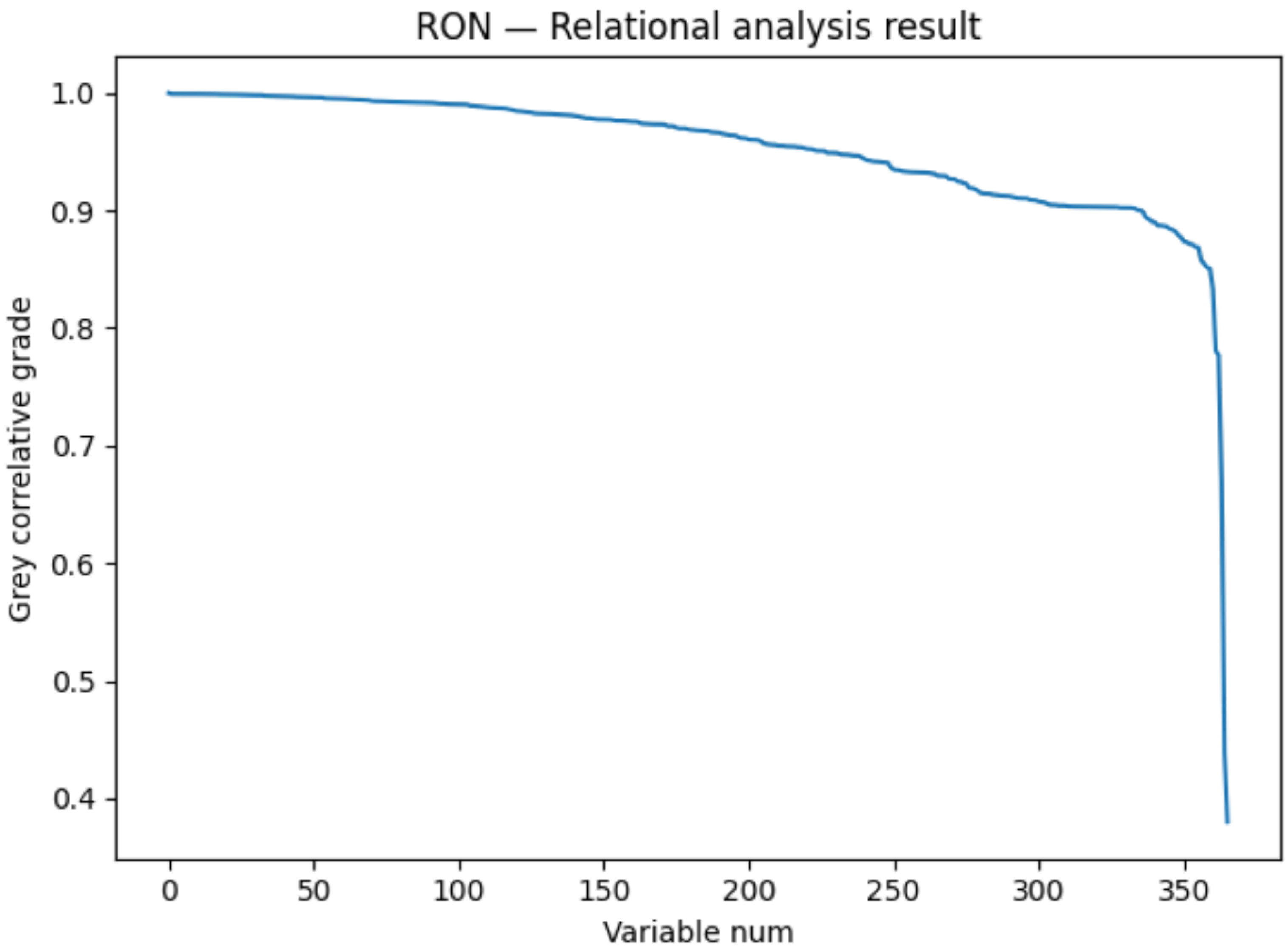
The idea of reducing dimensionality first and then modeling is often used in engineering problems. In order to screen out the main variables affecting the model, the grey correlation degree analysis was first used to screen out the variables with a greater correlation degree with RON to obtain representative variables. It was solved in Python to produce Figure 2.

After obtaining the grey correlative degree results of the independent variables and RON, we found that most of the non-operated variables in the independent variables are ranked in the top 150 of the grey correlative degree results, and most of the variables after the 150 are operated variables. This is also logical, because it is the non-operated variables that have a decisive impact on the change of RON, and the operated variables can only play an auxiliary role.

We can know from Figure 2 that the grey correlative degree of variables after the number of 150 began to decline significantly. If we choose more than 150 variables, this will not significantly increase the number of final independent variables. The variables after 150 are basically operating variables that have a relatively general impact on RON and they will have a strong relationship with the operated variables in the top 150 variables. These added variables will be replaced by the top 150 variables in the correlation analysis. So we finally adopted 150 as the demarcation point.

Perform Pearson correlation analysis on these 150 variables. Only one of them was kept in the strongly correlated variable group, identifying 19 variables that were representative and independent. The variable names and properties are shown in

Table 4. Main RON variables.

	Code	Property
1	Raw Material RON	Nonoperational Variable
2	Saturated Hydrocarbon	Nonoperational Variable
3	Aromatic Hydrocarbon	Nonoperational Variable
4	Density(20 °C)	Nonoperational Variable
5	S-ZORB.FC_2801.PV	Operational Variable
6	S-ZORB.TE_2103.PV	Operational Variable
7	S-ZORB.FT_9201.PV	Operational Variable
8	S-ZORB.SIS_TE_6010.PV	Operational Variable
9	S-ZORB.TC_1606.PV	Operational Variable
10	S-ZORB.FC_1203.PV	Operational Variable
11	S-ZORB.FT_9002.DACA	Operational Variable
12	S-ZORB.LT_9001.DACA	Operational Variable
13	S-ZORB.LC_5102.DACA	Operational Variable
14	S-ZORB.TE_2501.DACA	Operational Variable
15	S-ZORB.TE_5004.DACA	Operational Variable
16	S-ZORB.SIS_PT_2602.PV	Operational Variable
17	S-ZORB.PDC_2702.DACA	Operational Variable
18	S-ZORB.TXE_3201A.DACA	Operational Variable
19	S-ZORB.CAL.LINE.PV	Operational Variable

.

The correlation coefficients of these 19 variables are shown in

Table 5. The correlation coefficients of the major RON variables.

	1	2	3	4	5	6	7	8	9	10	11	12	13	14	15	16	17	18	19
1	1.000	−0.429	0.081	0.246	0.088	−1.002	−1.224	−1.018	0.065	0.378	−1.136	0.048	0.030	−1.059	0.185	−1.013	0.017	−1.174	0.075
2	−1.429	1.000	0.006	−1.138	−1.479	0.122	−1.059	0.123	−1.104	0.127	0.223	−1.192	−1.268	−1.112	−1.319	0.141	0.041	0.134	0.157
3	0.081	0.006	1.000	0.445	−1.111	−1.070	−1.001	0.170	0.060	−1.100	0.033	−1.094	−1.132	0.061	−1.133	−1.075	0.119	0.293	0.120
4	0.246	−1.138	0.445	1.000	−1.158	−1.128	−1.134	0.225	0.102	−1.017	0.133	−1.026	−1.147	−1.045	−1.085	−1.056	−1.007	0.273	0.109
5	0.088	−1.479	−1.111	−1.158	1.000	0.442	0.303	0.090	0.122	−1.005	0.201	0.235	0.335	0.272	0.453	0.149	0.377	−1.249	−1.365
6	−1.002	0.122	−1.070	−1.128	0.442	1.000	0.300	0.594	−1.226	0.423	0.388	0.031	−1.186	0.484	0.295	0.466	0.494	−1.092	0.014
7	−1.224	−1.059	−1.001	−1.134	0.303	0.300	1.000	0.336	0.022	−1.126	0.357	0.016	0.050	0.266	0.054	0.141	0.202	0.181	−1.002
8	−1.018	0.123	0.170	0.225	0.090	0.594	0.336	1.000	−1.097	0.265	0.491	−1.082	−1.273	0.361	0.160	0.276	0.227	0.370	0.355
9	0.065	−1.104	0.060	0.102	0.122	−1.226	0.022	−1.097	1.000	−1.104	0.060	0.182	0.264	−1.303	−1.014	−1.124	−1.082	−1.005	−1.182
10	0.378	0.127	−1.100	−1.017	−1.005	0.423	−1.126	0.265	−1.104	1.000	0.080	−1.061	−1.098	0.131	0.150	0.192	0.230	−1.144	0.278
11	−1.136	0.223	0.033	0.133	0.201	0.388	0.357	0.491	0.060	0.080	1.000	−1.002	−1.109	0.055	0.068	0.188	0.264	0.188	−1.058
12	0.048	−1.192	−1.094	−1.026	0.235	0.031	0.016	−1.082	0.182	−1.061	−1.002	1.000	0.276	−1.049	0.170	0.021	−1.047	−1.042	−1.003
13	0.030	−1.268	−1.132	−1.147	0.335	−1.186	0.050	−1.273	0.264	−1.098	−1.109	0.276	1.000	−1.243	0.128	−1.121	0.013	−1.225	−1.282
14	−1.059	−1.112	0.061	−1.045	0.272	0.484	0.266	0.361	−1.303	0.131	0.055	−1.049	−1.243	1.000	0.121	0.200	0.124	0.295	0.259
15	0.185	−1.319	−1.133	−1.085	0.453	0.295	0.054	0.160	−1.014	0.150	0.068	0.170	0.128	0.121	1.000	0.110	0.007	−1.029	−1.073
16	−1.013	0.141	−1.075	−1.056	0.149	0.466	0.141	0.276	−1.124	0.192	0.188	0.021	−1.121	0.200	0.110	1.000	0.162	−1.062	0.073
17	0.017	0.041	0.119	−1.007	0.377	0.494	0.202	0.227	−1.082	0.230	0.264	−1.047	0.013	0.124	0.007	0.162	1.000	−1.144	−1.252
18	−1.174	0.134	0.293	0.273	−1.249	−1.092	0.181	0.370	−1.005	−1.144	0.188	−1.042	−1.225	0.295	−1.029	−1.062	−1.144	1.000	0.383
19	0.075	0.157	0.120	0.109	−1.365	0.014	−1.002	0.355	−1.182	0.278	−1.058	−1.003	−1.282	0.259	−1.073	0.073	−1.252	0.383	1.000

.

As shown in Table 5, we found independence between variables. Therefore, these 19 variables are both representative and independent major variables affecting the gasoline RON.

The 14 main variables affecting S content were obtained by the same method. The variable names and properties are shown in

Table 6. Major S content variables.

	Code	Property
1	Raw Material S content	Nonoperational Variable
2	Raw Material RON	Nonoperational Variable
3	Olefin	Nonoperational Variable
4	Density(20 °C)	Nonoperational Variable
5	S-ZORB.FC_2801.PV	Operational Variable
6	S-ZORB.TE_2103.PV	Operational Variable
7	S-ZORB.FT_9201.PV	Operational Variable
8	S-ZORB.AT_1001.PV	Operational Variable
9	S-ZORB.AC_6001.PV	Operational Variable
10	S-ZORB.TC_1606.PV	Operational Variable
11	S-ZORB.TE_1203.PV	Operational Variable
12	S-ZORB.LC_5102.DACA	Operational Variable
13	S-ZORB.TE_5004.DACA	Operational Variable
14	S-ZORB.PDC_2702.DACA	Operational Variable

.

The correlation coefficients of these 14 variables are shown in

Table 7. The correlation coefficient of the main S content variables.

	1	2	3	4	5	6	7	8	9	10	11	12	13	14
1	1.000	0.475	0.393	0.191	0.174	−0.105	−0.118	0.431	0.138	0.113	0.052	0.244	0.091	0.088
2	0.475	1.000	0.366	0.246	0.088	−1.002	−1.224	0.219	−1.032	0.065	0.039	0.030	0.185	0.017
3	0.393	0.366	1.000	−1.039	0.485	−1.086	0.055	0.497	0.074	0.075	0.124	0.297	0.344	−1.083
4	0.191	0.246	−1.039	1.000	−1.158	−1.128	−1.134	−1.102	−1.020	0.102	0.025	−1.147	−1.085	−1.007
5	0.174	0.088	0.485	−1.158	1.000	0.442	0.303	0.485	0.135	0.122	0.260	0.335	0.453	0.377
6	−1.105	−1.002	−1.086	−1.128	0.442	1.000	0.300	0.101	0.005	−1.226	−1.265	−1.186	0.295	0.494
7	−1.118	−1.224	0.055	−1.134	0.303	0.300	1.000	0.091	0.029	0.022	−1.008	0.050	0.054	0.202
8	0.431	0.219	0.497	−1.102	0.485	0.101	0.091	1.000	0.104	0.110	0.114	0.259	0.191	0.190
9	0.138	−1.032	0.074	−1.020	0.135	0.005	0.029	0.104	1.000	0.093	0.034	0.091	−1.014	0.080
10	0.113	0.065	0.075	0.102	0.122	−1.226	0.022	0.110	0.093	1.000	0.329	0.264	−1.014	−1.082
11	0.052	0.039	0.124	0.025	0.260	−1.265	−1.008	0.114	0.034	0.329	1.000	0.246	0.135	0.042
12	0.244	0.030	0.297	−1.147	0.335	−1.186	0.050	0.259	0.091	0.264	0.246	1.000	0.128	0.013
13	0.091	0.185	0.344	−1.085	0.453	0.295	0.054	0.191	−1.014	−1.014	0.135	0.128	1.000	0.007
14	0.088	0.017	−1.083	−1.007	0.377	0.494	0.202	0.190	0.080	−1.082	0.042	0.013	0.007	1.000

.

As shown in Table 7, we found independence between variables. Therefore, these 14 variables were found to be both representative and independent main variables affecting S content.

3.2. Regression Analysis Model

First, the screened variables were taken as independent variables, the RON and S content of the product were taken as dependent variables to establish a multiple regression model, and the T-test and F-test were carried out to construct the product prediction model.

The logarithm model, inverse model, quadratic model, and combination model were transformed into linear regression separately in the form shown in Table 3.

Then, stepwise regression analysis was used for the linear model, logarithm model, inverse model, quadratic model, and combination model, separately. We used mean square error (MSE) as the evaluation criterion to determine the optimal case in each model. The optimal model of various models were obtained and their effects were recorded as shown in

Table 8. Functional form. MSE, mean square error; MAE, mean absolute error; $R^2$, coefficient of determination.

Model	Linear	Logarithm	Inverse	Quadratic	Combination
MSE	0.087	0.066	0.207	0.164	0.043
MAE	0.198	0.188	0.411	0.385	0.154
$R^2$	0.948	0.950	0.814	0.883	0.956

.

In this study, the MSE and MAE were selected as the measurement indexes of the prediction effect and prediction accuracy.

Mean square error:

$$MSE=\frac{1}{T}\sum _{t=1}^T{e}_t^2$$

(9)

Mean absolute error:

$$MAE=\frac{1}{T}\sum _{i=1}^T\left|e_t\right|$$

(10)

Then, we compared these models to obtain Figure 3.

As shown in Figure 3, both the MSE and MAE of the combination model were obviously the smallest, and $R^2$ was also the best, so we chose the combination model.

Based on the 325 sample data and using the main variables selected, the product RON was used as the predictive variable in the least squares method, and the variables with $P>1$ were eliminated by the t-test. The optimal model of combination model was obtained as

$$\begin{array}{c}y=0.7855+0.9958x_1-0.0103x_2+0.0004x_3-0.0032x_4+0.0012x_5-0.0046x_6\hfill \\ +0.2709ln{x}_7-0.2904ln{x}_8,\hfill \end{array}$$

(11)

which can be abbreviated to

$$y=a_0+\sum _{i=1}^6{a}_i{x}_i+\sum _{i=7}^8{a}_{i}ln{x}_i.$$

(12)

Similarly, the S content prediction model was obtained

$$z=-17.4300+0.0743t_1+0.115t_2-0.0368t_3+0.4615ln{t}_4+3.2104ln{t}_5-1.6812ln{t}_6.$$

(13)

That is,

$$z=c_0+\sum _{i=1}^3{c}_i{t}_i+\sum _{i=4}^6{c}_{i}ln{t}_i.$$

(14)

The symbolic descriptions of (12) and (14) were listed in

Table 9. Nomenclature.

Symbol	Meaning	Unit
y	Product RON	%
$x_1$	Raw Material RON	%
$x_2$	Saturated Hydrocarbon	%
$x_3$	S-ZORB.FC_2801.PV	Nm3/h
$x_4$	S-ZORB.TE_2103.PV	°C
$x_5$	S-ZORB.FT_9002.DACA	Nm3/h
$x_6$	S-ZORB.TE_5004.DACA	°C
$x_7$	S-ZORB.TE_2501.DACA	°C
$x_8$	S-ZORB.TXE_3201A.DACA	°C
z	Product S content	μg/g
$t_1$	Olefin	%
$t_2$	S-ZORB.TE_1203.PV	°C
$t_3$	S-ZORB.TE_5004.DACA	°C
$t_4$	Raw Material S content	μg/g
$t_5$	S-ZORB.FC_2801.PV	Nm3/h
$t_6$	S-ZORB.PDC_2702.DACA

.

It should be noted that $x_3$ and $t_5$ are the same variable, and $x_6$ and $t_3$ are also the same variable, so there is a certain correlation between the product RON and S content in the production process.

3.3. RON Loss Reduction Multi-Objective Optimization Model

Our goal was to optimize and adjust the operation plan of the FCC refinery desulfurization unit in the petrochemical plant to try to reduce the RON loss of gasoline by more than 30% under the premise of ensuring the desulfurization effect of gasoline products (S content being not more than 5 μg/g). In addition to the consideration of RON loss and operational risk, other factors such as the range of operational variables for the feasibility of S content operations were also considered. Only after the comprehensive measurement of all factors can the decision be more reasonable, which is a typical multi-objective optimization problem.

Combined with the actual situation, we ignored the minor factors. Therefore, we set up two objective functions: maximum RON loss reduction and minimum operational risk.

3.3.1. Objective Function 1

Taking the maximum RON loss reduction as the target, the corresponding function relation was obtained: RON loss = original RON loss – adjusted RON loss. If $R_0$ represents raw material RON, $R_1$ represents original product RON, and $Y_1$ represents adjusted product RON, then RON loss can be expressed as

$$R_0-R_1-(R_0-y_1)=y_1-R_1.$$

(15)

Substitute (12) into the above equation to obtain the objective function

$$max{a}_0+\sum _{i=1}^6{a}_i{x}_i+\sum _{i=7}^8{a}_{i}ln{x}_i-R_1.$$

(16)

3.3.2. Objective Function 2

In order to minimize the operational risk, we wrote the corresponding function relations. In the actual engineering operation process, for either manual adjustment or computer or machine control, each operation may pose certain risks: the less, the better. The original value of $x_i$ is denoted by $r_i$, and ${\mathsf{\Delta }}_i$ represents the maximum amount of change in the operation variable each time. The original value of $t_i$ is denoted by $s_i$, and ${\lambda }_i$ represents the maximum amount of change in the operation variable each time. As $x_1,x_2$ are not operation variables, $i=3,4,\dots ,8$ in the function expression for the number of operations of RON. As $t_1,t_4$ are not operation variables, $i=2,3,5,6$ in the function expression for the number of operations of S content. In addition, the number of operations that need to change but do not reach a multiple of ${\mathsf{\Delta }}_i$ and ${\lambda }_i$ should be rounded up, even if it is less than ${\mathsf{\Delta }}_i$ and ${\lambda }_i$. Then, the objective function with the smallest number of operations can be expressed as

$$min\sum _{i=3}^8⌈\frac{\left|x_i-r_i\right|}{{\mathsf{\Delta }}_i}⌉+\sum _{i=2}^3⌈\frac{\left|t_i-s_i\right|}{{\lambda }_i}⌉+\sum _{i=5}^6⌈\frac{\left|t_i-s_i\right|}{{\lambda }_i}⌉.$$

(17)

However, the number of operations is related to the variable, and the relationship containing the variable needs to be rounded up. This was difficult to achieve in the solver process, so we needed to remove the integer symbol. After removing the integer symbol, this expression expresses the relative modification range. Similarly, the smaller the relative modification range, the fewer the operation times, and the lower the operation risk. Therefore, the function expression of objective function 2 can be expressed as

$$min\sum _{i=3}^8\frac{\left|x_i-r_i\right|}{{\mathsf{\Delta }}_i}+\sum _{i=2}^3\frac{\left|t_i-s_i\right|}{{\lambda }_i}+\sum _{i=5}^6\frac{\left|t_i-s_i\right|}{{\lambda }_i}.$$

(18)

3.3.3. Constraint Condition 1

First, since optimization was carried out, the product RON after the optimized operation had to be larger than the previous product RON $R_1$; otherwise, the optimization would be meaningless. In addition, the product RON was transformed from the raw material RON, so the product RON after optimized operation could not be greater than the raw material RON $R_0$. Therefore, the constraint condition1 was

$$R_1\le a_0+\sum _{i=1}^6{a}_i{x}_i+\sum _{i=7}^8{a}_{i}ln{x}_i\le R_0.$$

(19)

3.3.4. Constraint Condition 2

Our goal was to reduce the RON loss of gasoline to more than 30% under the condition that the S content was no more than 5 μg/g, so we needed to restrict the S content to less than or equal to 5 μg/g. Therefore, the constraint condition 2 was

$$c_0+\sum _{i=1}^3{c}_i{t}_i+\sum _{i=4}^6{c}_{i}ln{t}_i\le 5.$$

(20)

3.3.5. Constraint Condition 3

Due to process requirements and operation experience, each operation variable has its operating range, with $[l_i,u_i]$ denoting the operating range corresponding to $x_i$, and $[L_i,U_i]$ denoting the operating range corresponding to $t_i$. In addition, $x_1,x_2,t_1,t_4$ are not operation variables, so $i=3,4,\dots ,8$ for $x_i$ and $i=2,3,5,6$ for $t_i$. Therefore, the corresponding constraint condition 3 is

$$l_i\le x_i\le u_i,i=3,4,\dots ,8.$$

(21)

$$L_i\le t_i\le U_i,i=2,3,5,6.$$

(22)

It ensures the robustness of the model. Because as long as the variable meets the constraints of the scope of operation, the operability of the solution can be guaranteed.

3.3.6. Constraint Condition 4

As $x_3$ and $t_5$ are the same variable, and $x_6$ and $t_3$ are also the same variable, the constraint condition 4 is

$$x_3=t_5,$$

(23)

$$x_6=t_3.$$

(24)

3.3.7. Constraint Condition 5

As $x_1,x_2,t_1,t_4$ are not operation variables, they are equal to their original value and do not change, so the constraint condition 5 is

$$x_i=r_i,i=1,2,$$

(25)

$$t_i=s_i,i=1,4.$$

(26)

By sorting out the above objective function and constraint conditions, the multi-objective nonlinear optimization model of the RON loss reduction is expressed as

$$\begin{array}{c}max{a}_0+{\displaystyle \sum _{i=1}^6}{a}_i{x}_i+{\displaystyle \sum _{i=7}^8}{a}_{i}ln{x}_i-R_1,\hfill \\ min{\displaystyle \sum _{i=3}^8}\frac{\left|x_i-r_i\right|}{{\mathsf{\Delta }}_i}+{\displaystyle \sum _{i=2}^3}\frac{\left|t_i-s_i\right|}{{\lambda }_i}+{\displaystyle \sum _{i=5}^6}\frac{\left|t_i-s_i\right|}{{\lambda }_i},\hfill \\ s.t.\left\{\begin{array}{c}{R}_1\le a_0+{\displaystyle \sum _{i=1}^6}{a}_i{x}_i+{\displaystyle \sum _{i=7}^8}{a}_{i}ln{x}_i\le R_0,\hfill \\ c_0+{\displaystyle \sum _{i=1}^3}{c}_i{t}_i+{\displaystyle \sum _{i=4}^6}{c}_{i}ln{t}_i\le 5,\hfill \\ l_i\le x_i\le u_i,i=3,4,\dots ,8,\hfill \\ L_i\le t_i\le U_i,i=2,3,5,6,\hfill \\ x_3=t_5,\hfill \\ x_6=t_3,\hfill \\ x_i=r_i,i=1,2,\hfill \\ t_i=s_i,i=1,4.\hfill \end{array}\right.\hfill \end{array}$$

(27)

Although the RON loss reduction multi-objective optimization model was established, we found that there were two urgent problems to be addressed before solving: The dual objective needed to be changed into a single objective and the absolute values needed to be removed, and nonlinear programming needed to be changed into linear programming. Then, we used Python to solve the model.

Here, RON loss reduction was an obviously important main goal, so risk minimization was set as a constraint condition to transform the multi-objective problem into a single-objective problem. We set the maximum value of the constraint range corresponding to operational risk as T, then the RON loss reduction multi-objective nonlinear optimization model was transformed into the single-objective nonlinear model.

There were also absolute values in the model, so the nonlinear optimization was changed into linear optimization by introducing new variables to the absolute value. We introduced the non-negative variable $x_i^1,x_i^2,i=3,4,\dots ,8,$ and $t_i^1,t_i^2,i=2,3,5,6.$

Let

$$\left\{\begin{array}{c}\left|x_i-r_i\right|=x_i^1+x_i^2,i=3,4,\dots ,8,\hfill \\ x_i-r_i=x_i^1-x_i^2,i=3,4,\dots ,8,\hfill \\ x_i^1,x_i^2\ge 0,i=3,4,\dots ,8,\hfill \\ \left|t_i-s_i\right|=t_i^1+t_i^2,i=2,3,5,6,\hfill \\ t_i-r_i=t_i^1-t_i^2,i=2,3,5,6,\hfill \\ t_i^1,t_i^2\ge 0,i=2,3,5,6.\hfill \end{array}\right.$$

(28)

Thus,

$$x_i=x_i^1-x_i^2+r_i,i=3,4,\dots ,8,$$

(29)

$$t_i=t_i^1-t_i^2+s_i,i=2,3,5,6.$$

(30)

In conclusion, the multi-objective nonlinear optimization model is transformed into

$$\begin{array}{c}max{a}_0+a_1{x}_1+a_2{x}_2+{\displaystyle \sum _{i=3}^6}{a}_i(x_i^1-x_i^2+r_i)+{\displaystyle \sum _{i=7}^8}{a}_{i}ln(x_i^1-x_i^2+r_i)-R_1\hfill \\ s.t.\left\{\begin{array}{c}{\displaystyle \sum _{i=3}^8}\frac{x_i^1+x_i^2}{{\mathsf{\Delta }}_i}+{\displaystyle \sum _{i=2}^3}\frac{t_i^1+t_i^2}{{\lambda }_i}+{\displaystyle \sum _{i=5}^6}\frac{t_i^1+t_i^2}{{\lambda }_i}\le T,\hfill \\ a_0+a_1{x}_1+a_2{x}_2+{\displaystyle \sum _{i=3}^6}{a}_i\left(x_i^1-x_i^2+{\gamma }_i\right)+{\displaystyle \sum _{i=7}^8}{a}_{i}ln\left(x_i^1-x_i^2+{\gamma }_i\right)\ge R_1,\hfill \\ a_0+a_1{x}_1+a_2{x}_2+{\displaystyle \sum _{i=3}^6}{a}_i\left(x_i^1-x_i^2+{\gamma }_i\right)+{\displaystyle \sum _{i=7}^8}{a}_{i}ln\left(x_i^1-x_i^2+{\gamma }_i\right)\le R_0,\hfill \\ c_0+c_1{t}_1+c_{4}ln{t}_4+{\displaystyle \sum _{i=2}^3}{c}_i\left(t_i^1-t_i^2+s_i\right)+{\displaystyle \sum _{i=5}^6}{c}_{i}ln\left(t_i^1-t_i^2+s_i\right)\le 5,\hfill \\ x_i^1-x_i^2+r_i\ge l_i,i=3,4,\cdots ,8,\hfill \\ x_i^1-x_i^2+r_i\le u_i,i=3,4,\cdots ,8,\hfill \\ t_i^1-t_i^2+s_i\ge L_i,i=2,3,5,6,\hfill \\ t_i^1-t_i^2+s_i\le U_i,i=2,3,5,6,\hfill \\ x_3^1-x_3^2+r_3=t_5^1-t_5^2+s_5,\hfill \\ x_6^1-x_3^2+r_6=t_3^1-t_3^2+s_3,\hfill \\ x_1=r_1,\hfill \\ x_2=r_2,\hfill \\ t_1=s_1,\hfill \\ t_4=s_4,\hfill \\ x_i^1,x_i^2\ge 0,i=3,4,\cdots ,8,\hfill \\ t_i^1,t_i^2\ge 0,i=2,3,5,6.\hfill \end{array}\right.\hfill \end{array}$$

(31)

We used SLSQP in Python to solve the model. Some adjustments to the sample with a loss reduction of 30% were in

Table 10. Adjustments to the sample with a loss reduction of 30%.

Sample	${\mathit{R}}_0$	${\mathit{R}}_1$	Adjusted ${\mathit{R}}_1$	Loss of Decline	N	${\mathit{N}}_{\mathit{max}}$
1	90.600	89.220	89.778	40.4%	126	45
2	90.500	89.320	89.684	30.9%	126	48
3	90.700	89.320	89.897	41.8%	126	50
4	90.400	89.020	89.613	43.0%	125	46
5	89.600	88.320	88.819	39.0%	125	35
6	91.000	89.590	90.218	44.5%	126	40
7	90.400	89.200	89.628	35.6%	126	37
8	90.500	89.200	89.744	41.9%	126	40
9	90.400	89.300	89.639	30.8%	125	43
10	90.200	88.800	89.440	45.7%	126	34
11	90.200	88.900	89.421	40.1%	127	38
12	90.200	88.900	89.420	40.0%	126	29
13	89.200	87.700	88.415	47.6%	124	34
14	86.800	85.400	86.014	43.8%	125	36
15	87.800	86.100	86.947	49.8%	127	52
16	88.400	86.700	87.539	49.4%	125	49
18	88.000	86.490	87.112	41.2%	127	54
20	88.800	87.590	87.957	30.3%	127	48
21	88.100	86.590	87.250	43.7%	126	41
23	89.600	87.990	88.742	46.7%	125	48
24	89.000	87.590	88.139	39.0%	125	47
25	89.300	87.890	88.455	40.1%	125	45
26	89.200	87.690	88.364	44.6%	127	41
27	88.700	87.290	87.851	39.8%	125	46
29	89.700	88.290	88.835	38.7%	124	38
30	89.200	87.990	88.354	30.1%	126	38

.

Where, N represents total number of adjustments, $N_{max}$ denotes the number of adjustments of the variable with the largest number of adjustments.

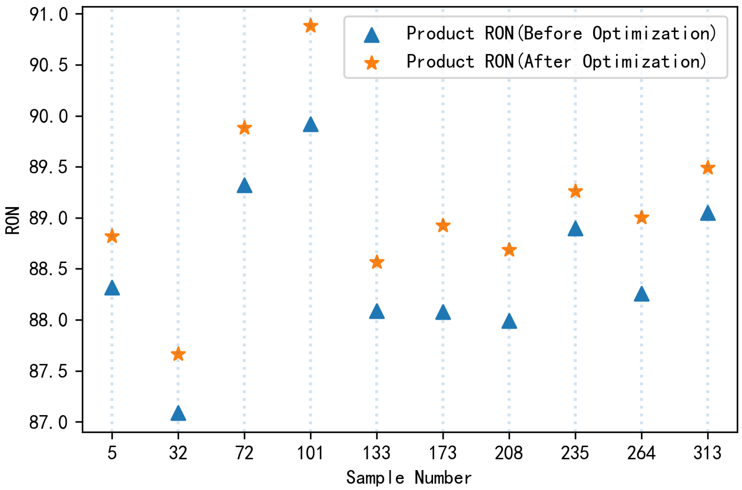
Note that in the model, the larger the T, the more samples can reach the 30% loss reduction. The T value is usually set according to practical experience. In this study, it was set to 120. After calculation, we found that 245 of the 325 samples achieved 30% loss reduction, that is, 78.2% reached the target, indicating that a good effect was achieved.

We randomly selected 10 samples with a loss reduction greater than 30% and compared the product RON before and after optimization to obtain Figure 4.

The operation scheme of the main variables of some samples whose loss reduction was greater than 30% is provided in

Table 11. Operation scheme of some samples.

Variable	State	5	32	72	101	133	173	208	235	264	313
$x_3$	Original	649.341	649.651	652.010	650.353	648.496	698.963	748.972	752.160	735.709	849.255
	New	688.459	689.943	673.658	693.481	680.361	714.732	780.464	781.161	776.337	879.403
$x_4$	Original	427.132	425.923	421.054	427.430	426.620	426.620	428.348	424.131	425.028	424.969
	New	410.000	410.000	410.000	410.000	410.000	410.000	410.000	410.000	410.000	410.000
$x_5$	Original	401.752	414.780	514.261	377.199	452.605	550.321	448.482	464.489	411.784	454.247
	New	650.000	650.000	650.000	650.000	650.000	650.000	650.000	650.000	650.000	650.000
$x_6$	Original	64.960	61.005	64.001	67.419	56.947	64.552	61.733	67.671	50.020	66.559
	New	40.000	40.000	40.000	40.000	40.000	40.000	40.000	40.000	40.000	40.000
$x_7$	Original	215.227	216.749	167.173	210.013	225.360	190.146	174.339	202.865	206.900	171.674
	New	250.000	250.000	222.727	246.926	234.211	240.377	224.549	246.049	250.000	215.856
$x_8$	Original	366.214	413.725	410.599	426.298	402.040	431.804	311.955	377.150	359.226	396.256
	New	357.878	394.361	410.599	426.298	349.257	431.711	311.955	377.150	326.958	396.256
$t_2$	Original	30.114	35.913	32.248	33.647	29.621	33.853	32.254	31.203	34.217	34.640
	New	30.114	35.913	32.248	33.647	29.621	33.853	32.254	31.203	34.217	34.640
$t_3$	Original	64.960	61.005	64.001	67.419	56.947	64.552	61.733	67.671	50.020	66.559
	New	40.000	40.000	40.000	40.000	40.000	40.000	40.000	40.000	40.000	40.000
$t_5$	Original	649.341	649.651	652.010	650.353	648.496	698.963	748.972	752.160	735.709	849.255
	New	688.459	689.943	673.658	693.481	680.361	714.732	780.464	781.161	776.337	879.403
$t_6$	Original	27.151	26.585	27.375	26.097	26.352	31.078	30.957	24.442	29.668	27.450
	New	27.151	26.585	27.375	26.097	26.352	31.078	30.957	24.442	29.668	27.450

.

It can be seen from Table 11 that $t_2$ and $t_6$ need not to be adjusted, while $x_4$,$x_5$,$x_6$,$t_3$ are optimal in the fixed state regardless of which sample.

Their feature descriptions are summarized into

Table 12. Features of variables in the optimal operation scheme.

Feature	Variable	Value
Stable	$x_4$	410
	$x_5$	650
	$x_6=t_3$	40
Unstable	$x_3=t_5$	/
	$x_7$	/
	$x_8$	/
Unadjusted	$t_2$	/
	$t_6$	/

.

From the above results, we can briefly summarize the optimal operation scheme. For any sample, adjust S-ZORB.TE_2103.PV, S-ZORB.FT_9002.DACA, S-ZORB.TE_5004.DACA to 410, 650, 40 respectively. S-ZORB.FC_2801.PV, S-ZORB.TE_2501.DACA, S-ZORB. TXE_3201A.DACA need be adjusted differently depending on the initial state. And there is no need to adjust S-ZORB.TE_1203.PV, S-ZORB.PDC_2702.DACA.

4. Conclusions

This research was conducted on the basis of four years’ data from Sinopec Gaoqiao Petrochemical, including 325 samples, 354 operation sites of the FCC gasoline refining desulfurization unit, and 367 variables. Data preprocessing was first carried out on these data. Then, the main variables were selected from 367 operational variables through grey correlation analysis and Pearson correlation analysis. Then, according to the selected major variables, the RON loss prediction model was established by multiple regression analysis, and the model was verified. The same method was used to predict S content. Notably, $x_3$ and $t_5$ are the same variable and $x_6$ and $t_3$ are also the same variable, so there is a certain correlation between product RON and S content in the production process. In the end, under the condition that the S content would be no more than 5 μg/g, the reduction in RON loss was more than 30%, and the operating conditions after the optimization of the major variables were obtained.

We presented a new systematic method for determining an optimal operation scheme for minimising RON loss and operational risks. For the data with highly nonlinear and strongly coupled, it was preprocessed first, dimension reduction and regression prediction were carried out, finally an optimization model was established to solve the optimization scheme. With the system we’ve built, just input data that needs to be improved, operation scheme to reduce RON loss can be output.

This system can be applied to the dimensionality reduction, prediction, and operation scheme optimization of data with the same properties. The regression model in the paper can be used to fields related to forecasting, such as medical care, geography, finance, and industry. The optimization model is suitable for optimizing model parameters, seeking extreme values, and so on. The optimization model is based on the regression model, which can well solve most of the problems that require modeling or optimization due to data clutter, such as the establishment of a bank credit information system, the measurement of the effectiveness of biomedical reagents, etc.

References

Gaffney, J.S.; Marley, N.A.; Martin, R.S.; Dixon, R.W.; Reyes, L.G.; Popp, C.J. Potential air quality effects of using ethanol-gasoline fuel blends: A field study in Albuquerque, New Mexico. Environ. Sci. Technol.1997, 31, 3053–3061. [Google Scholar] [CrossRef]
Nelson, P.; Quigley, S. The hydrocarbon composition of exhaust emitted from gasoline fuelled vehicles. Atmos. Environ.1984, 18, 79–87. [Google Scholar] [CrossRef]
Barcia, P.S.; Silva, J.A.; Rodrigues, A.E. Adsorption dynamics of C5–C6 isomerate fractions in zeolite beta for the octane improvement of gasoline. Energy Fuels2010, 24, 1931–1940. [Google Scholar] [CrossRef]
Ahmadlou, M.; Rezakazemi, M. Computational fluid dynamics simulation of moving-bed nanocatalytic cracking process for the lightening of heavy crude oil. J. Porous Media2018, 21. [Google Scholar] [CrossRef]
Samolada, M.; Baldauf, W.; Vasalos, I. Production of a bio-gasoline by upgrading biomass flash pyrolysis liquids via hydrogen processing and catalytic cracking. Fuel1998, 77, 1667–1675. [Google Scholar] [CrossRef]
Shih, S.; Owens, P.; Palit, S.; Tryjankowski, D. Mobil’s OCTGAIN™ Process: FCC Gasoline Desulfurization Reaches a New Performance Level. In Proceedings of the NPRA 1999 Annual Meeting, San Antonio, TX, USA, 21–23 March 1999. [Google Scholar]
Zainullin, R.; Koledina, K.; Akhmetov, A.; Gubaidullin, I. Kinetics of the catalytic reforming of gasoline. Kinet. Catal.2017, 58, 279–289. [Google Scholar] [CrossRef]
Ayanoğlu, A.; Yumrutaş, R. Production of gasoline and diesel like fuels from waste tire oil by using catalytic pyrolysis. Energy2016, 103, 456–468. [Google Scholar] [CrossRef]
Wang, W.; Wang, S.; Wang, Y.; Liu, H.; Wang, Z. A new approach to deep desulfurization of gasoline by electrochemically catalytic oxidation and extraction. Fuel Process. Technol.2007, 88, 1002–1008. [Google Scholar] [CrossRef]
Nocca, J.; Cosyns, J.; Debuisschert, Q.; Didillon, B. The domino interaction of refinery processes for gasoline quality attainment. In Proceedings of the NPRA Annual Meeting, San Antonio, TX, USA, 26–28 March 2000. [Google Scholar]
Halbert, T.R.; Greeley, J.P. Technology options for meeting low sulfur targets. In Proceedings of the NPRA Annual Meeting, AM-00-11, San Antonio, TX, USA, 26–28 March 2000. [Google Scholar]
Nelson, P.; George, J.; Edward, J. Meeting gasoline pool sulfur and octane targets with ISAL (r) process. In Proceedings of the NPRA Annual Meeting, AM-00-52, San Antonio, TX, USA, 23–25 March 2000. [Google Scholar]
Jiang, H.; Huang, S. Eight-lump reaction kinetic model for the maximizing isoparaffin process for cleaning gasoline and enhancing propylene yield. Energy Fuels2016, 30, 10770–10776. [Google Scholar] [CrossRef]
Sadighi, S.; Zahedi, S.; Hayati, R.; Bayat, M. Studying Catalyst Activity in an Isomerization Plant to Upgrade the Octane Number of Gasoline by Using a Hybrid Artificial-Neural-Network Model. Energy Technol.2013, 1, 743–750. [Google Scholar] [CrossRef]
Hamadi, A.S. Selective additives for improvement of gasoline octane number. Tikrit J. Eng. Sci.2010, 17, 22–35. [Google Scholar]
Daly, S.R.; Niemeyer, K.E.; Cannella, W.J.; Hagen, C.L. Predicting fuel research octane number using Fourier-transform infrared absorption spectra of neat hydrocarbons. Fuel2016, 183, 359–365. [Google Scholar] [CrossRef] [Green Version]
Santikunaporn, M.; Alvarez, W.E.; Resasco, D.E. Ring contraction and selective ring opening of naphthenic molecules for octane number improvement. Appl. Catal. A Gen.2007, 325, 175–187. [Google Scholar] [CrossRef]
Diwekar, U.M.; Rubin, E. Stochastic modeling of chemical processes. Comput. Chem. Eng.1991, 15, 105–114. [Google Scholar] [CrossRef] [Green Version]
Te Braake, H.; Van Can, H.; Verbruggen, H. Semi-mechanistic modeling of chemical processes with neural networks. Eng. Appl. Artif. Intell.1998, 11, 507–515. [Google Scholar] [CrossRef]
Rice, R.G.; Do, D.D. Applied Mathematics and Modeling for Chemical Engineers; John Wiley & Sons: Hoboken, NJ, USA, 2012. [Google Scholar]
Tränkle, F.; Zeitz, M.; Ginkel, M.; Gilles, E. PROMOT: A modeling tool for chemical processes. Math. Comput. Model. Dyn. Syst.2000, 6, 283–307. [Google Scholar] [CrossRef]
McBride, K.; Sundmacher, K. Overview of surrogate modeling in chemical process engineering. Chem. Ing. Tech.2019, 91, 228–239. [Google Scholar] [CrossRef] [Green Version]
Kulov, N.; Gordeev, L. Mathematical modeling in chemical engineering and biotechnology. Theor. Found. Chem. Eng.2014, 48, 225–229. [Google Scholar] [CrossRef]
Ni, J.; Zhou, Y.; Li, S. Hamiltonian Monte Carlo-Based D-Vine Copula Regression Model for Soft Sensor Modeling of Complex Chemical Processes. Ind. Eng. Chem. Res.2020, 59, 1607–1618. [Google Scholar] [CrossRef]
Xuan, Z.; Wei, G.; Ni, Z.; Zhang, J. Decoupling Offloading Decision and Resource Allocation via Deep Reinforcement Learning and Sequential Least Squares Programming. In Proceedings of the International Conference on Communications and Networking, Shanghai, China, 20–21 November 2020; pp. 554–566. [Google Scholar]
Sultana, N.; Hossain, S.; Taher, S.; Khan, A.; Razzak, S.; Haq, B. Modeling and optimization of non-edible papaya seed waste oil synthesis using data mining approaches. S. Afr. J. Chem. Eng.2020, 33, 151–159. [Google Scholar] [CrossRef]
Arendt, K.; Jradi, M.; Wetter, M.; Veje, C.T. Modestpy: An open-source python tool for parameter estimation in functional mock-up units. In Proceedings of the American Modelica Conference, Cambridge, MA, USA, 9–10 October 2018. [Google Scholar]
Kalogirou, S.A. Optimization of solar systems using artificial neural-networks and genetic algorithms. Appl. Energy2004, 77, 383–405. [Google Scholar] [CrossRef]
Kumar, M.; Husain, M.; Upreti, N.; Gupta, D. Genetic Algorithm: Review and Application; SSRN 3529843; SSRN: Rochester, NY, USA, 2010. [Google Scholar]
Whitley, D. A genetic algorithm tutorial. Stat. Comput.1994, 4, 65–85. [Google Scholar] [CrossRef]
Liu, X.; Liu, Y.; He, X.; Xiao, M.; Jiang, T.