Article

Novel Numerical Spiking Neural P Systems with a Variable Consumption Strategy

1
Academy of Management Science, Business School, Shandong Normal University, Jinan 250000, China
2
College of Business, The University of Texas at San Antonio, San Antonio, TX 78249, USA
*
Author to whom correspondence should be addressed.
Processes 2021, 9(3), 549; https://doi.org/10.3390/pr9030549
Submission received: 10 February 2021 / Revised: 14 March 2021 / Accepted: 15 March 2021 / Published: 20 March 2021
(This article belongs to the Special Issue Modeling, Simulation and Design of Membrane Computing System)

Abstract

:
A novel variant of NSN P systems, called numerical spiking neural P systems with a variable consumption strategy (NSNVC P systems), is proposed. Like the spiking rules consuming spikes in spiking neural P systems, NSNVC P systems introduce a variable consumption strategy by modifying the form of the production functions used in NSN P systems. Similar to the delay feature of the spiking rules, NSNVC P systems introduce a postponement feature into the production functions. The execution of the production functions in NSNVC P systems is controlled by two, i.e., polarization and threshold, conditions. Multiple synaptic channels are used to transmit the charges and the production values in NSNVC P systems. The proposed NSNVC P systems are a type of distributed parallel computing models with a directed graphical structure. The Turing universality of the proposed NSNVC P systems is proved as number generating/accepting devices. Detailed descriptions are provided for NSNVC P systems as number generating/accepting devices. In addition, a universal NSNVC P system with 66 neurons is constructed as a function computing device.

1. Introduction

Membrane computing is a class of distributed parallel-computing models introduced by Păun [1], which is inspired by the structure and function of living cells and their cooperation in tissues, organs, and biological neural networks. These computing models are called P systems or membrane systems [2]. There are three main types of P systems, i.e., cell-like P systems, tissue-like P systems and neural-like P systems. Specifically, the cell-like P systems were proposed based on the hierarchical structure of biological membranes in cells, the tissue-like P systems were abstracted from the communication and cooperation of cells in biological tissues, and the neural-like P systems were inspired by the facts that neurons communicate with each other by firing short electrical impulses or spikes.
Spiking neural P (SN P) systems, proposed by Ionescu et al. [3], are a main form of neural-like P systems. A SN P system consists of a network of neurons connected together in a directed graph and can be regarded as the third generation of neural network models. In the past few years, many variants of SN P systems have been proposed and studied as being inspired by various biological activities and/or by combining methods and ideas in computer science and mathematics. SN P systems with astrocytes, having excitatory and inhibitory influences on synapses, were discussed by Păun [4] and Pan et al. [5]. SN P systems with anti-spikes were constructed by Pan and Păun [6] with anti-spikes abstracted from inhibitory impulses that participate in spiking and forgetting rules and annihilate spikes when they are in the same neuron. Motivated by the biological phenomenon that each neuron has a positive or negative charge, SN P systems with polarizations are established by Wu et al. [7]. SN P systems with rules on synapses were proposed by Song et al. [8], which is different from most P systems where the rules are located in neurons. Considering the biological fact that a synapse has one or more chemical channels, Peng et al. [9] and Song et al. [10] studied SN P systems with multiple channels. Wang et al. [11] and Zeng et al. [12] proposed SN P systems with weights and thresholds, respectively. Recently, coupled neural P systems [13] and dynamic threshold neural P systems [14] have also been proposed one after another. Most SN P systems are synchronous under the control of a global clock, but many SN P systems are asynchronous [15,16,17]. Many variants of SN P systems have been proven to be Turing universal as number generating/accepting devices [18,19,20], language generating devices [21,22], and function computing devices [23,24,25].
In SN P systems with polarizations (PSN P systems) [7], the polarization associated with neurons can also control the firing of the spiking rules. Hence, the regular expressions are no longer the only conditions controlling the firing of the spiking rules. Three types of polarizations, i.e., positive, neutral, and negative, corresponding to three kinds of electrical charges, i.e., +, 0 and −, respectively, exist in PSN P systems. Specifically, each neuron contains an initial charge and each spiking rule also has a charge. A rule can apply only when the charge of the rule is the same as the charge of the neuron where the rule is located.
Different from the above P systems, numerical P (NP) systems are another special type of P systems [26], having a similar architecture to those of many cell-like P systems. NP systems are composed of hierarchically arranged membranes and compartments formed by adjacent membranes. Numerical variables are configured in the compartment instead of being treated as multisets of chemical objects as used in most P systems. The variables evolve through programs consisting of production functions and repartition protocols, which is fundamentally different from most P systems that use multiset rewriting rules to evolve. In order to more effectively control the application of the programs, many variants of NP systems, such as enzymatic NP systems [27], NP systems with production thresholds [28], and NP systems with Boolean conditions [29] have been proposed.
These biologically inspired P systems have both advantages and disadvantages for solving real-world problems. Most P systems are distributed parallel computing models, in which each neuron can act as an independent processor, and neurons communicate through the spikes represented by unique symbols. The evolution rules in the P systems are usually applied non-deterministically and in maximally parallel, i.e., the order in which the rules are applied is random and all possible rules must be performed in each step of the computation. Therefore, the P systems have the characteristics of simple representation of knowledge, non-determinism, and parallelism. These advantages make them very attractive for solving real-world problems such as image processing [30,31,32], robots [33,34], fault detection [35,36,37] and data clustering [38,39,40]. Under the control of a global clock, the application of rules in the P systems is synchronized. However, from a computational point of view, the synchronization of the process leads to higher costs. SN P systems and their variants encode information through spikes in neurons and neurons can only fire when the number of spikes reaches a certain value, which makes these systems discrete computing models. However, practical applications involve numerical representation of information and require precise and quantitative modeling of data. Therefore, it is difficult for these systems to solve these practical problems. In order to overcome this difficulty, Wu et al. [41] proposed numerical spiking neural P (NSN P) systems by introducing numerical variables and production functions used in NP systems into SN P systems. In this way, NSN P systems are equipped with numerical capabilities, making them more capable of solving real-world problems.
A novel variant of NSN P systems, called numerical spiking neural P systems with a variable consumption strategy (NSNVC P systems), is proposed in this study. The Turing universality of NSNVC P systems is investigated as number generating/accepting devices. Moreover, a universal NSNVC P system with 66 neurons is also constructed as a function computing device. NSN P systems use continuous production functions to replace the usual spiking rules. After the execution of a production function, the values of the variables involved in the production function will all return to 0 in NSN P systems. The variable resetting may cut down the controlling ability and the operating efficiency of NSN P systems. In addition, NSN P systems lose the firing feature of SN P systems and the real biological systems. Hence, it is necessary and feasible for NSNVC P systems to make improvements. In order to regain the firing feature, each production function is assigned a threshold in NSNVC P systems. Considering that polarizations can control the firing of spiking rules, NSNVC P systems use polarizations and threshold to simultaneously control the execution of the production functions. As in NSN P systems, NSNVC P systems also use multiple synaptic channels to transmit the charges and production values to other neurons.
Compared with NSN P systems, the improvements in NSNVC P systems are as follows.
  • By modifying the form of the production functions, NSNVC P systems adopt a new variable consumption strategy, in which the values of the variables involved will have a prescribed consumption rate without all being set to 0 after a production function execution.
  • In addition to assigning a threshold to each production function to control the firing of the neurons, polarizations of the neurons, where the production functions are located, are also used to control production function executions in NSNVC P systems. Therefore, both the polarization and the threshold can control the execution of a production function.
  • The proposed NSNVC P systems also introduce postponement features and multiple synaptic channels to reduce the complexity and the number of computing units, i.e., neurons, of the systems.
Some variants of P systems with their abbreviations and full names cited in this work are listed in Table 1. Comparisons of performances of the proposed NSNVC P systems with some of these variants of P systems listed in Table 1 are given in Section 5.
The main motivation of this work is to design NSNVC P systems to improve the computation performance of NSN P systems. In NSNVC P systems, a new variable consumption strategy is proposed, which not only improves the computation mechanism, but also increases the controlling ability of NSN P systems. In addition, the improvement in the computation performance of NSN P systems will be investigated when both polarization and threshold are used to control the execution of the production functions. The improvement in computation performance of NSN P systems is made by enhancing their controlling ability, improving their operating efficiency, and reducing the number of neurons used. As a result, the new variant of NSN P systems, i.e., the NSNVC P systems, is expected to be more suitable for solving real-world problems.
The rest of this paper is organized as follows. A formal definition and an illustrative example of NSNVC P systems are presented in Section 2. The proof of the universality of NSNVC P systems as number accepting/generating devices is given in Section 3. Section 4 investigates the universality of NSNVC P systems as function computing devices. Section 5 draws conclusions and outlines future research directions.

2. NSNVC P Systems

A formal definition of the proposed NSNVC P systems is presented and notations used in NSNVC P systems are defined in this section. An example is then given to facilitate the understanding of the proposed NSNVC P systems. The set of natural numbers, the set of positive integers, and the set of integers are represented by N , N + and Z , respectively.

2.1. The Definition of NSNVC P Systems

A NSNVC P system composed of m neurons is represented by the tuple Π = ( L , σ 1 , σ 2 , , σ m , s y n , i n , o u t ) , where:
  • L N + represents the set of channel labels.
  • σ 1 , σ 2 , , σ m represents m neurons with the form σ i = ( α i , L i , V a r i , Pr f i , V a r i ( 0 ) ) , for 1 i m . The specifics of a neuron are given below.
    (a)
    α i { + , 0 , } refers to the initial charge of neuron σ i , where +, 0 and − indicate the positive, neutral and negative polarizations, respectively.
    (b)
    L i L is a finite set of channel labels of neuron σ i , indicating its synaptic channels. A synaptic channel of neuron σ i may involve one or more synapses connecting neuron σ i to other neurons and a synapse may be involved in a number of synaptic channels.
    (c)
    V a r i = { x q , i | 1 q k i } is the set of variables in neuron σ i .
    (d)
    V a r i ( 0 ) = { x q , i ( 0 ) | x q , i ( 0 ) Z ,   1 q k i } is the set of initial values of the variables in neuron σ i .
    (e)
    Pr f i represents a finite set of production functions associated with neuron σ i . The form of a production function is α / f h , i ( x l , i , , x k i , i ) | T h C h ; β ; d ; ( l ) , where α , β { + , 0 , } ; l is the channel label indicating the synaptic channel of neuron σ i associated with the function; 1 h | Pr f i | is used to distinguish the production functions contained in neuron σ i ; C h N is the consumption rate of the variables when the production function f h , i . executes; T h N + refers to the threshold at which the production function can execute; and d 0 indicates the postponement future of the production function. If d = 0 , the form of production function is simplified to α / f h , i ( x l , i , , x k i , i ) | T h C h ; β ; ( l ) .
  • s y n = { ( i , j , l ) } { 1 , 2 , , m } × { 1 , 2 , , m } × L with i j is the set of synapses among the m neurons with their channel labels, where ( i , j , l ) s y n means that neuron σ i connects to neuron σ j via synaptic channel l . If a synapse connects from neuron σ i to neuron σ j , neuron σ i is called a presynaptic neuron of neuron σ j and neuron σ j is called a postsynaptic neuron of neuron σ i .
  • i n indicates the input neuron.
  • o u t indicates the output neuron.
Numerical variables in NSNVC P systems are represented by x with subscripts. Specifically, the first subscript of a variable indicates the order of the variable among all the variables in the same neuron, and the second subscript is the label of the neuron. For example, variable x q , i represents variable q in neuron σ i . The value of variable x q , i at time t is expressed as x q , i ( t ) for 1 q k i and 1 i m . Usually, the values of the variables are real numbers. This work restricts the values of the variables to an interval of integers in order to simplify the computation, although NSNVC P systems have the computational capability of processing real umbers. The subscripts of the production functions are used in the same ways as those of the numerical variables, e.g., production function f h , i represents function h in neuron σ i . In fact, production functions can be any mathematical functions. However, NSNVC P systems are able to achieve the same capabilities as Turing machines under the condition of only using linear functions.
Two forms of, i.e., non-threshold f h , i ( x l , i , , x k i , i ) and threshold f h , i ( x l , i , , x k i , i ) | T h , production functions exist in NSN P systems. When T h min ( x 1 , i ( t ) , , x k , i ( t ) ) , the threshold production function f h , i ( x l , i , , x k i , i ) | T h can execute, i.e., the neuron where the production function f h , i ( x l , i , , x k i , i ) | T h is located can fire. However, the neuron where the non-threshold production function f h , i ( x l , i , , x k i , i ) is located lost the firing feature. In addition, the values of all variables involved in the production function, whether threshold or non-threshold, will be reset to 0 immediately after the function execution.
The execution of production functions in NSNVC P systems will be described below. At time t , the execution of a production function α / f h , i ( x l , i , , x k i , i ) | T h C h ; β ; d ; ( l ) in neuron σ i can be roughly divided into three, i.e., comparison, production and distribution, stages.
  • Comparison stage: Only when neuron σ i contains just charge α and the current values of the variables x 1 , i ( t ) , , x k i , i ( t ) involved in the production function are all equal to the threshold T h , i.e., x 1 , i ( t ) = = x k , i ( t ) = T h , the production function α / f h , i ( x l , i , , x k i , i ) | T h C h ; β ; d ; ( l ) can apply. Otherwise, the production function cannot apply.
  • Production stage: If production function α / f h , i ( x l , i , , x k i , i ) | T h C h ; β ; d ; ( l ) can be applied at time t , then its production value p r v h , i ( t ) = f h , i ( x l , i , , x k i , i ) is calculated based on the current values of the variables x 1 , i ( t ) , , x k i , i ( t ) .
  • Distribution stage: The distribution of the production value p r v h , i ( t ) and a charge β is based on the repartition protocol, which is stated in the following. The production value p r v h , i ( t ) and the charge β are transmitted to all postsynaptic neurons σ j of neuron σ i through synaptic channel l at time t + d . If d = 0 , the transmission happens immediately at time t . If d 1 , then neuron σ i is dormant, i.e., cannot fire nor receive new production values, at time t ,   t + 1 ,   ,   t + d 1 . At time t + d , neuron σ i becomes active again and the transmission occurs. In particular, the value received by neuron σ j will be immediately passed to its variables, which will increase or decrease the values of the variables.
Based on the variable consumption strategy, after the execution of production function α / f h , i ( x l , i , , x k i , i ) | T h C h ; β ; d ; ( l ) , all variables involved will “consume” a value of C h , while the variables not involved will keep their current values. Moreover, the condition C h min ( x 1 , i ( t ) , , x k , i ( t ) ) must be satisfied before the execution of the production function. If neuron σ i receives several production values at time t , p r v ( t ) will be the sum of all these production values. Then, the value of variable x q , i in neuron σ i at time t + 1 is updated according to (1) in the following:
x q , i ( t + 1 ) = { p r v ( t ) + x q , i ( t ) C h , if   x q , i   is   involved   in   f h , i p r v ( t ) + x q , i ( t ) , if   x q , i   is   not   involved   in   f h , i
At the same time, neuron σ i also receives the charges delivered by all its presynaptic neurons. The charge calculation rules are as follows:
  • Multiple positive, neutral and negative charges will degenerate to a single charge of the same kind.
  • A positive charge plus a negative charge will produce a neutral charge.
  • A positive or negative charge will not change after a neutral charge is added to it.
In NSNVC P systems, at most one production function can execute in a single neuron at each time moment, and all neurons in system Π work in parallel. At a certain time moment, when more than one production function can satisfy the condition to execute in a neuron, one production function in the neuron will be chosen non-deterministically to apply.
A configuration of system Π is represented by the polarizations of all neurons and the current values of all the variables contained therein. At time t , the configuration of system Π is represented by a vector t = ( [ α 1 , x 1 , 1 ( t ) , , x k i , 1 ( t ) ] , , [ α m , x 1 , m ( t ) , , x k i , m ( t ) ] ) , where α i { + , 0 , } indicates the charge of neuron σ i , and x q , i ( t ) Z is the current value of x q , i , for 1 q k i and 1 i m . Therefore, the initial configuration of the system is 0 = ( [ α 1 , x 1 , 1 ( 0 ) , , x k i , 1 ( 0 ) ] , , [ α m , x 1 , m ( 0 ) , , x k i , m ( 0 ) ] ) .
A transition of system Π is defined as an update from one configuration to another, i.e., t t + 1 This transition is realized by the system by applying production functions in parallel. Starting from the initial configuration 0 , a series of finite or infinite transitions of system Π , i.e., 0 1 s with s N , is called a system calculation. When system Π progresses to a configuration where no production functions can apply, the system halts and the calculation terminates.
A NSNVC P system Π can be used as a number generating device, also called a number generator, and can generate a number n . In this case, the output neuron σ o u t is used to output the computation result. The number generated by system Π is related to the moments when the output neuron σ o u t fires. Specifically, if t 1 and t 2 are the first two time moments when the output neuron emits a nonzero value to the environment, then the time interval t 2 t 1 is defined as the computation result, i.e., the number generated by system Π . In this way, the entire system needs a global clock to pace the time for all neurons, and system Π is assumed to start working at time t = 1 . All computation results produced by system Π are represented by N 2 ( Π ) , where the subscript 2 represents the interval between the first two time moments when the output neuron fires.
A NSNVC P system Π can also be used as a number accepting device, also called a number acceptor. In this case, the input neuron σ i n is used to introduce numbers into the system. The output neuron is removed from the system when it is used as a number accepting device. The number n N + introduced into the system is encoded by the time interval between the first two time moments when the input neuron fires. When the system computation stops, the number n is accepted by the system. The set of all numbers accepted by system Π is represented by N a c c ( Π ) .
The family of all sets of numbers generated/accepted by NSNVC P systems is represented by N η c h p I N S N P ( p o l y λ ( r ) ) , where η { 2 , a c c } , c h p indicates that the system uses at most p charges, and p o l y λ ( r ) indicates that each production function is a polynomial with a degree of at most λ 0 and with at most r 0 variables.

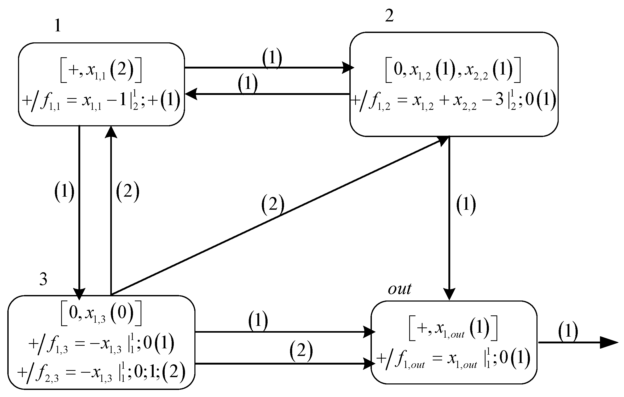
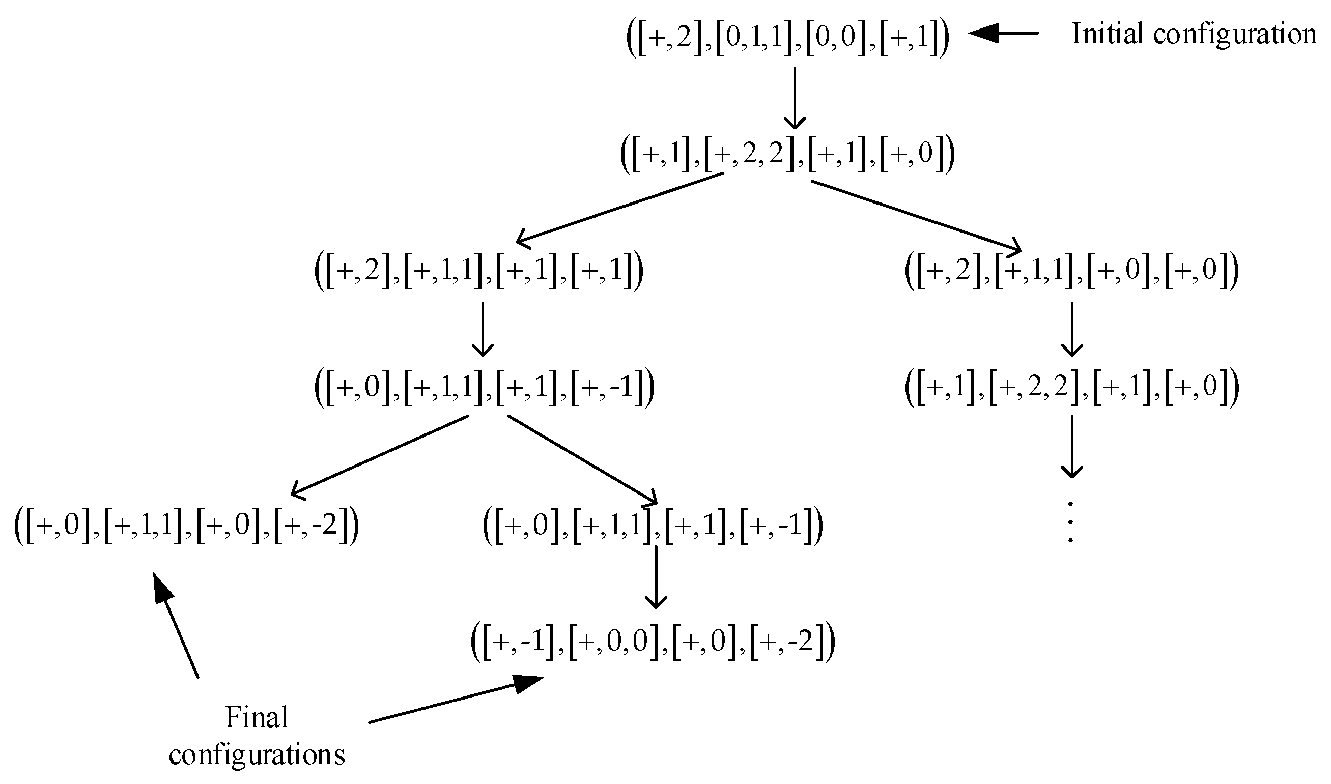
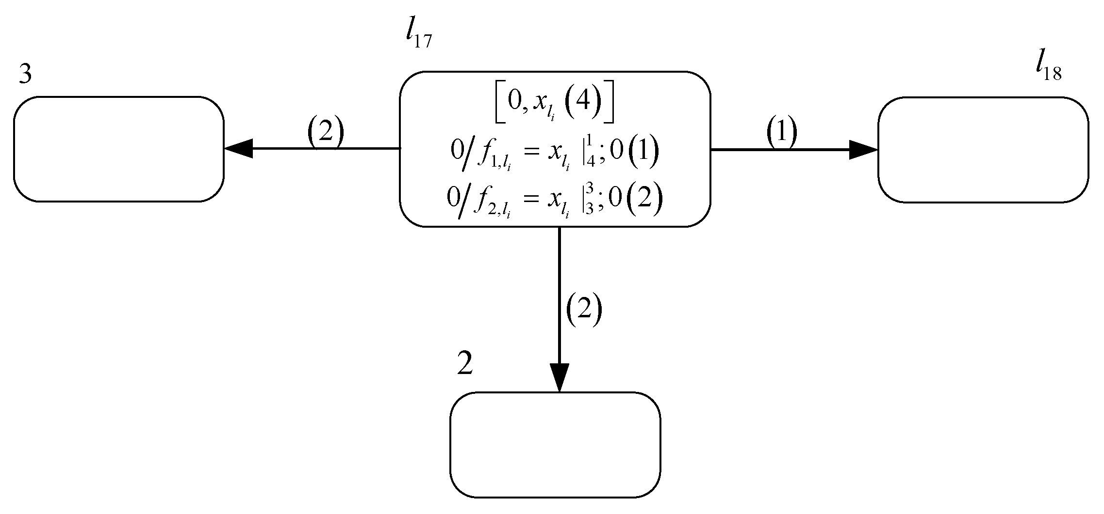
2.2. An Illustrative Example

The example system Π e x shown in Figure 1 is used to clarify the components, the definitions, and the functions of NSNVC P systems. System Π e x consists of four neurons σ 1 , σ 2 , σ 3 and σ o u t , represented by four rectangles and labeled with 1, 2, 3, and out, respectively. Each neuron contains one or more production functions and a list, where the first item in the list is the initial charge of the neuron, and the other items are the variables with the initial values in parentheses. A neuron may contain multiple variables. The output neuron σ o u t is used to transmit calculation results to the environment. A synapse is represented by an arrow connecting two neurons. A synaptic channel of a neuron is represented by the channel label marked on one or more synapses connecting from the neuron to other neurons.
Apparently, the initial configuration of system Π e x is 0 = ( [ α 1 , x 1 , 1 ( 0 ) ] , [ α 2 , x 1 , 2 ( 0 ) , x 2 , 2 ( 0 ) ] , [ α 3 , x 1 , 3 ( 0 ) ] , [ α 4 , x 1 , 4 ( 0 ) ] ) = ( [ + , 2 ] , [ 0 , 1 , 1 ] , [ 0 , 0 ] , [ + , 1 ] ) . Since neuron σ 1 contains the initial charge + and the initial value of variable x 1 , 1 is equal to the threshold 2, the production function + / f 1 , 1 = x 1 , 1 1 | 2 1 ; + ; ( 1 ) can be enabled. At time t = 1 , without a postponement feature, i.e., d = 0 , production function + / f 1 , 1 = x 1 , 1 1 | 2 1 ; + ; ( 1 ) executes and neuron σ 1 immediately transmits a value of 1 and a positive charge to neurons σ 2 and σ 3 via synaptic channel (1). According to the variable consumption strategy, the value of variable x 1 , 1 will decrease by 1 after production function + / f 1 , 1 = x 1 , 1 1 | 2 1 ; + ; ( 1 ) executes. Similarly, production function + / f 1 , o u t = x 1 , o u t | 1 1 ; 0 ; ( 1 ) in output neuron σ o u t also meets the execution condition at time t = 1 , so that output neuron σ o u t sends the first nonzero value of 1 to the environment and the value of variable x 1 , o u t becomes 0. However, neurons σ 2 and σ 3 cannot fire because their functions do not satisfy their execution conditions.
Due to the firing of neuron σ 1 , neurons σ 2 and σ 3 both receive a positive charge and the values of variables x 1 , 2 , x 2 , 2 and x 3 , 1 all increase by 1. Therefore, the configuration of system Π e x at time t = 1 becomes 1 = ( [ + , 1 ] , [ + , 2 , 2 ] , [ + , 1 ] , [ + , 0 ] ) . Accordingly, production function + / f 1 , 2 = x 1 , 2 + x 2 , 2 3 | 2 1 ; + ; ( 1 ) of neuron σ 2 satisfies the execution condition and neuron σ 2 sends a value of 1 and a neutral charge to neurons σ o u t and σ 1 via synaptic channel (1) at time t = 2 . From the charge calculation rules, the transmission of neutral charges does not have any effect on the polarization of the postsynaptic neurons. Therefore, the polarizations of neurons σ o u t and σ 1 do not change but the values of variables x 1 , 1 and x 1 , o u t increase by 1.
The two production functions + / f 1 , 3 = x 1 , 3 | 1 1 ; 0 ; ( 1 ) and + / f 2 , 3 = x 1 , 3 | 1 1 ; 0 ; 1 ; ( 2 ) of neuron σ 3 also satisfy their execution conditions at time t = 2 , but only one of them will be selected non-deterministically for application. Assuming production function + / f 1 , 3 = x 1 , 3 | 1 1 ; 0 ; ( 1 ) is selected, neuron σ 3 sends a value of −1 and a neutral charge to neuron σ o u t via synaptic channel (1). Since neurons σ 2 and σ 3 send values of 1 and −1, respectively, to neuron σ o u t at the same time, the value of variable x 1 , o u t in neuron σ o u t does not change. Therefore, neuron σ o u t will not fire. The configuration of system Π e x at time t = 2 becomes 2 = ( [ + , 2 ] , [ + , 1 , 1 ] , [ + , 0 ] , [ + , 0 ] ) .
At time t = 3 , only production function + / f 1 , 1 = x 1 , 1 1 | 2 1 ; + ; ( 1 ) in neuron σ 1 meets the execution condition, so that neuron σ 1 sends a positive charge and a value of 1 to neurons σ 2 and σ 3 . As a result of this transmission, only the values of the variables change. Thus, the configuration of system Π e x at time t = 3 becomes 3 = ( [ + , 1 ] , [ + , 2 , 2 ] , [ + , 1 ] , [ + , 0 ] ) . Obviously, the configuration of system Π e x at time t = 3 is the same as that at time t = 1 . If the production function + / f 1 , 3 = x 1 , 3 | 1 1 ; 0 ; ( 1 ) in neuron σ 3 continues to execute, system Π e x will loop between these two configurations indefinitely.
Suppose production function + / f 2 , 3 = x 1 , 3 | 1 1 ; 0 ; 1 ; ( 2 ) in neuron σ 3 is chosen to execute at time t = 2 t + 2 for t N . However, since production function + / f 2 , 3 = x 1 , 3 | 1 1 ; 0 ; 1 ; ( 2 ) needs to postpone the execution for a time span of d = 1 , it will execute at time t = 2 t + 3 . Thus, the configuration of system Π e x at time t = 2 t + 2 becomes 2 t + 2 = ( [ + , 2 ] , [ + , 1 , 1 ] , [ + , 1 ] , [ + , 1 ] ) . At time t = 2 t + 3 , neuron σ o u t fires and sends the second nonzero value to the environment. At the same time, production functions in neurons σ 1 and σ 3 also satisfy their execution conditions. Therefore, neuron σ 3 sends a neutral charge and a value of −1 to neurons σ 1 , σ 2 and σ o u t via synaptic channel (2), and neuron σ 1 transmits a positive charge and a value of 1 to neurons σ 2 and σ 3 via synaptic channel (1). Thus, the configuration of system Π e x at time t = 2 t + 3 becomes 2 t + 3 = ( [ + , 0 ] , [ + , 1 , 1 ] , [ + , 1 ] , [ + , 1 ] ) .
At time t = 2 t + 4 , neuron σ 3 faces two choices again, but neuron σ o u t will not fire no matter which production function is applied. The final configuration of system Π e x becomes 2 t + 4 = ( [ + , 0 ] , [ + , 1 , 1 ] , [ + , 0 ] , [ + , 2 ] ) if production function + / f 1 , 3 = x 1 , 3 | 1 1 ; 0 ; ( 1 ) is selected, or becomes 2 t + 5 = ( [ + , 1 ] , [ + , 0 , 0 ] , [ + , 0 ] , [ + , 2 ] ) if production function + / f 2 , 3 = x 1 , 3 | 1 1 ; 0 ; 1 ; ( 2 ) is selected.
Figure 2 shows the configuration dynamics of system Π e x . Each configuration in turn involves variables in neurons σ 1 , σ 2 , σ 3 and σ o u t . The number generated by system Π e x is the time interval between the first two time moments when the output neuron σ o u t sends non-zero values to the environment, i.e., ( 2 t + 3 ) 1 = 2 t + 2 , with t N . In other words, system Π e x can generate even numbers other than 0. Hence, system Π e x can be used as a number generating device.

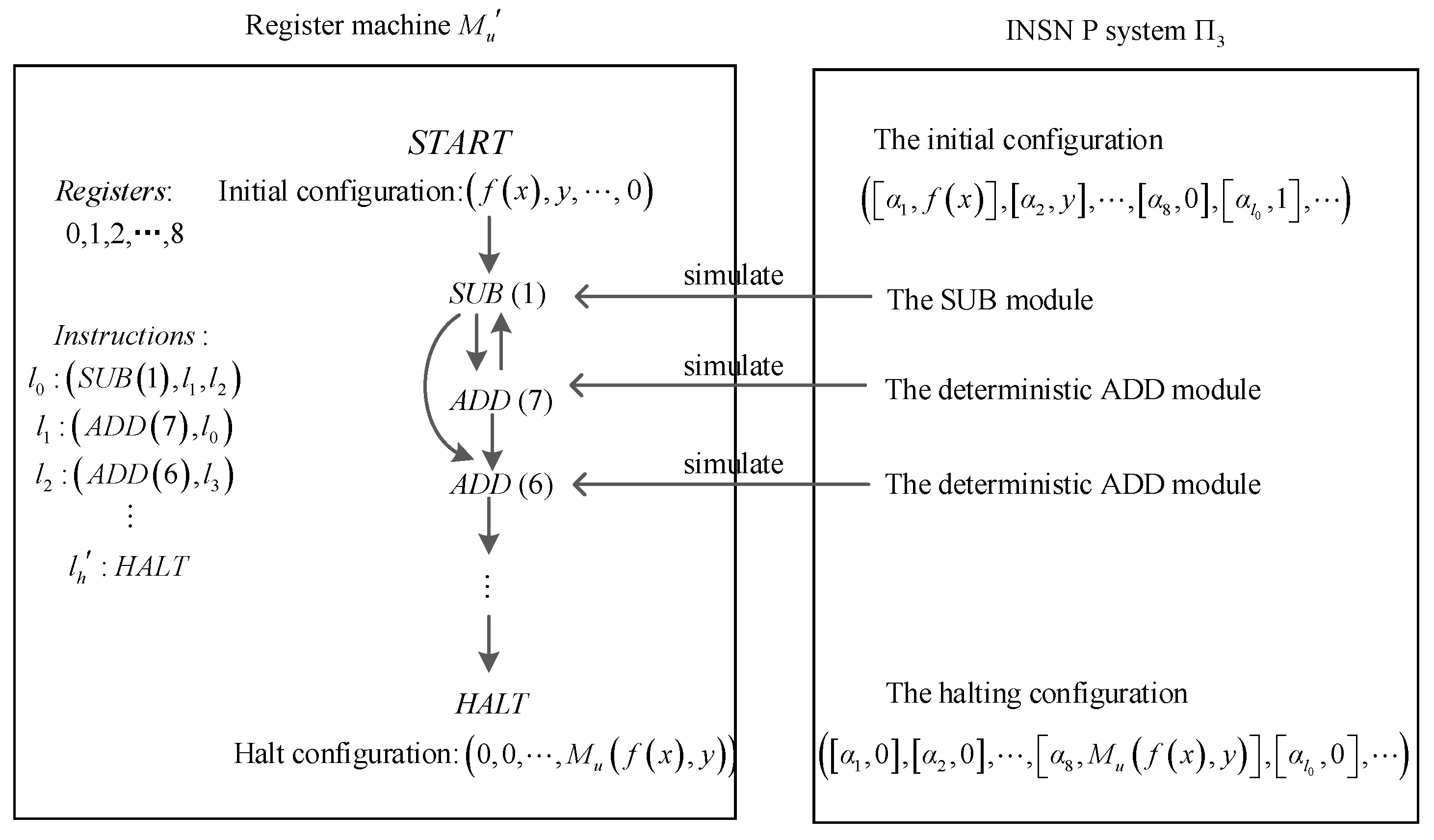
3. Turing Universality of NSNVC P Systems as Number Generating/Accepting Devices

The focus of this section is on the computation power of NSNVC P systems as number generating/accepting devices. Specifically, the Turing universality of NSNVC P systems is proved as number generators and number acceptors by simulating register machines, i.e., NSNVC P systems can generate/accept all recursively enumerable sets of numbers. The family of all recursively enumerable sets of numbers is represented by NRE.
A register machine is usually represented as a five-tuple M = ( m ¯ , H , l 0 , l h , I ) , where:
  • m ¯ is the number of registers.
  • H represents a limited set of instruction labels.
  • l 0 , l h H correspond to the START and HALT instruction labels, respectively.
  • I is a set of labeled instructions. The instructions in I have the following three forms:
    (a)
    ADD instructions l i : ( A D D ( r ) , l j , l k ) , whose function is to add 1 to the value in register r , and move non-deterministically to one of the instructions with labels l j and l k ;
    (b)
    SUB instructions l i : ( S U B ( r ) , l j , l k ) , whose function is to subtract 1 from the value of register r , and then go to the instruction marked by l j if the number stored in r is nonzero, or go to the instruction marked by l k otherwise;
    (c)
    The HALT instruction l h : H A L T , whose function is to terminate the operation of the register machine.

3.1. NSNVC P Systems as Number Generating Devices

The register machine M can generate a set of numbers N ( M ) in the generating mode. When all the registers are empty, machine M continuously executes a series of instructions starting from the initial instruction l 0 . When M reaches the HALT instruction, the number stored in the first register is considered to be the number generated by M . In addition, it is well known that register machines can characterize the N R E family.
Theorem 1.
N 2 c h 2 N S N V C   P ( p o l y 1 ( 1 ) ) = N R E .
Proof. 
Based on the characterization of N R E , the proof of the inclusion N R E N 2 c h 2 N S N V C   P ( p o l y 1 ( 1 ) ) can be obtained by simulating nondeterministic register machines running in the generating mode, while the converse inclusion is achieved by the Turing-Church thesis [41]. □
A NSNVC P system Π 1 is constructed to simulate the register machine M . Generally, register 1 is used as an output register, and the number that it stores is never decremented during the computation. Specifically, system Π 1 contains three types of modules, i.e., an ADD module to simulate the ADD instruction, a SUB module to simulate the SUB instruction, and a FIN module to output the computation result.
Considering that each production function of any neuron in system Π 1 is only related to one variable, the first index of the variables is omitted and only the second index identifying the neuron housing the variable is retained. For example, the variable x 1 , i in neuron σ i is simplified to x i . Similarly, when a neuron contains only one production function, its first index will also be omitted. Although the value of a variable x i changes dynamically, it is always an integer during the entire computation process of system Π 1 , i.e., x i ( t ) Z with t N . In addition, all production functions in system Π 1 are polynomial functions.
In order to simulate M correctly, there is a correspondence between the elements, i.e., the neurons, of system Π 1 and the elements, i.e., the registers and the instructions, of M . Each register r of M corresponds to a neuron σ r in system Π 1 . If register r stores a number n 0 , then the value of variable x r in neuron σ r is 3 n . Each labeled instruction is also associated with a neuron, e.g., an instruction with label l i is related to a unique neuron σ l i . Moreover, some auxiliary neurons are also introduced into system Π 1 .
The values of all the variables are 0 in the initial configuration of system Π 1 . System Π 1 starts the simulation of M when variable x l 0 in neuron σ l 0 is assigned a value of 4. Similarly, the ADD module and the SUB module will simulate the corresponding instructions l i : ( A D D ( r ) , l j , l k ) and l i : ( S U B ( r ) , l j , l k ) , respectively, once the value of variable x l i in neuron σ l i is equal to 4 in the simulation process. System Π 1 starts to simulate the HALT instruction l h : H A L T and the entire simulation terminates when variable x l h in neuron σ l h receives a value of 4 at any time moment. Then the FIN module is activated to output the computation results.
To better clarify the whole process of using system Π 1 to simulate M , the ADD, SUB, and FIN modules are shown step by step to simulate the relevant instructions of M .

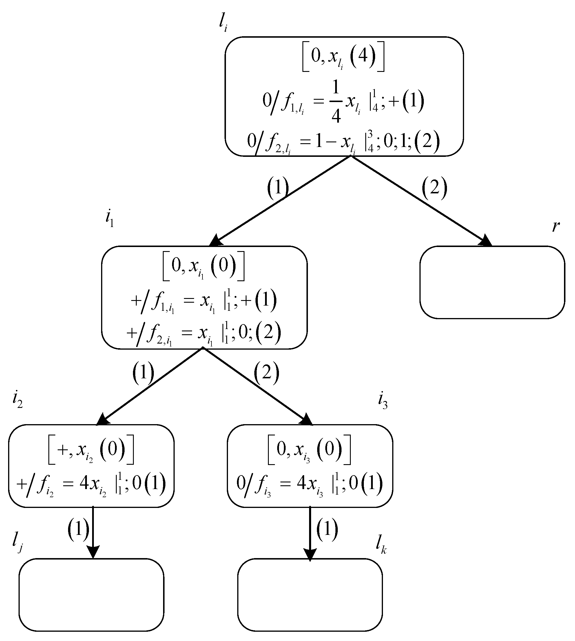
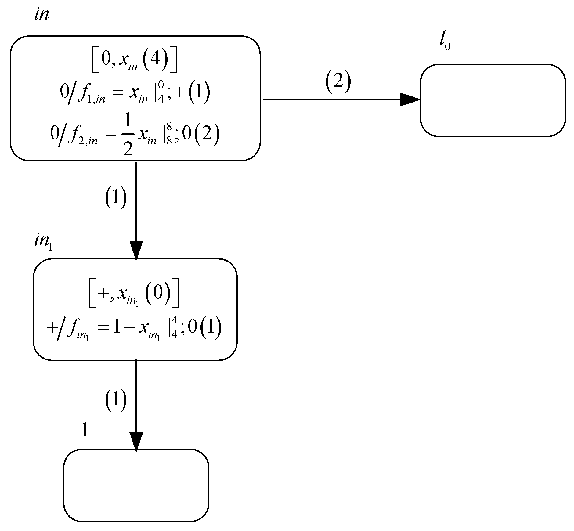
3.1.1. Module ADD—Simulating an ADD Instruction

Figure 3 displays the architecture of the ADD module and the state of the neurons it contains. When neuron σ l i receives a value of 4 at a certain time moment t = t , system Π 1 then starts simulating the ADD instruction l i : ( A D D ( r ) , l j , l k ) . At this moment, the values of all the variables except x r in neuron σ r are all 0. The configuration of system Π 1 at time t = t is t = ( [ 0 , 4 ] , [ 0 , 3 n ] , [ 0 , 0 ] , [ 0 , 0 ] , [ 0 , 0 ] , [ 0 , 0 ] , [ 0 , 0 ] ) , which involves neurons σ l i , σ r , σ i 1 , σ i 2 , σ i 3 , σ l j , and σ l k .
At time t = t + 1 , both production functions 0 / f 1 , l i = 1 4 x l i | 4 1 ; + ; ( 1 ) and 0 / f 2 , l i = 1 x l i | 4 3 ; 0 ; 1 ; ( 2 ) can execute. Because production function 0 / f 2 , l i = 1 x l i | 4 3 ; 0 ; 1 ; ( 2 ) has a postponement feature, production function 0 / f 1 , l i = 1 4 x l i | 4 1 ; + ; ( 1 ) will execute first. Thus, neuron σ l i fires to transmit a positive charge and a value of 1 to neuron σ i 1 via synaptic channel ( 1 ) . After production function 0 / f 1 , l i = 1 4 x l i | 4 1 ; + ; ( 1 ) executes, the value of variable x l i will decrease by 1 according to the variable consumption strategy. Thus, the configuration of system Π 1 at time t = t + 1 becomes t + 1 = ( [ 0 , 3 ] , [ 0 , 3 n ] , [ + , 1 ] , [ 0 , 0 ] , [ 0 , 0 ] , [ 0 , 0 ] , [ 0 , 0 ] ) .
After a one-step delay, i.e., at time t = t + 2 , production function 0 / f 2 , l i = 1 x l i | 4 3 ; 0 ; 1 ; ( 2 ) executes and neuron σ l i transmits a neutral charge and a value of −3 to neuron σ r via synaptic channel ( 2 ) , indicating that system Π 1 has completed the operation of adding 1 to the value stored in register r . According to the charge calculation rules, the neutral charge has no effect on the polarization of a neuron, so that the descriptions of the neutral charges will be omitted below. Meanwhile, neuron σ i 1 fires by executing one of the production functions + / f 1 , i 1 = x i 1 | 1 1 ; + ; ( 1 ) and + / f 2 , i 1 = x i 1 | 1 1 ; 0 ; ( 2 ) non-deterministically.
  • If production function + / f 1 , i 1 = x i 1 | 1 1 ; + ; ( 1 ) is selected for execution at time t = t + 2 , then neuron σ i 1 sends a positive charge and a value of 1 to neuron σ i 2 . As a result, the polarization of neuron σ i 2 becomes positive and variable x i 2 gets a value of 1. Therefore, the configuration of system Π 1 at time t = t + 2 becomes t + 2 = ( [ 0 , 0 ] , [ 0 , 3 3 n ] , [ + , 0 ] , [ + , 1 ] , [ 0 , 0 ] , [ 0 , 0 ] , [ 0 , 0 ] ) . At time t = t + 3 , production function + / f i 2 = 4 x i 2 | 1 1 ; 0 ; ( 1 ) satisfies the execution condition, so that neuron σ i 2 transmits a value of 4 to neuron σ l j , causing system Π 1 to start simulating the instruction with label l j in M .
  • If production function + / f 2 , i 1 = x i 1 | 1 1 ; 0 ; ( 2 ) is selected for execution at time t = t + 2 , neuron σ i 1 sends a value of 1 to neuron σ i 3 . Therefore, the configuration of system Π 1 at time t = t + 2 becomes t + 2 = ( [ 0 , 0 ] , [ 0 , 3 3 n ] , [ + , 0 ] , [ + , 0 ] , [ 0 , 1 ] , [ 0 , 0 ] , [ 0 , 0 ] ) . At time t = t + 3 , neuron σ i 3 transmits a value of 4 to neuron σ l k , causing system Π 1 to start simulating the instruction with label l k in M .
As described above, the ADD module shown in Figure 3 can correctly simulate the ADD instruction l i : ( A D D ( r ) , l j , l k ) of M . Specifically, system Π 1 is activated when variable x l i receives the value of 4, and then 1 is added to the value stored in register r . Subsequently, an instruction, l j or l k , is selected non-deterministically for simulation.

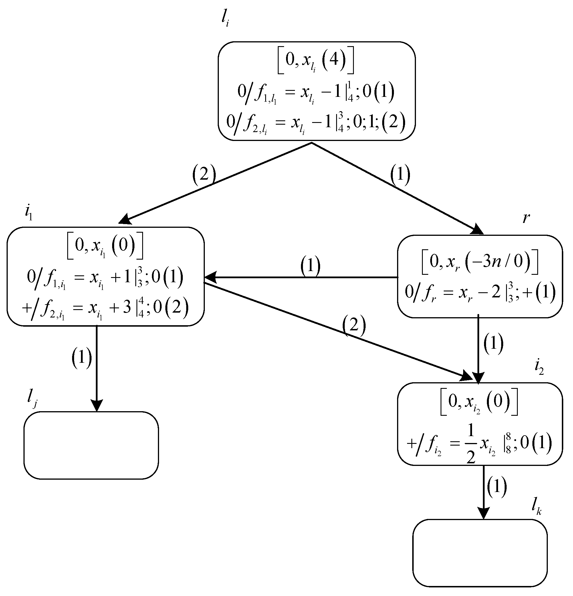
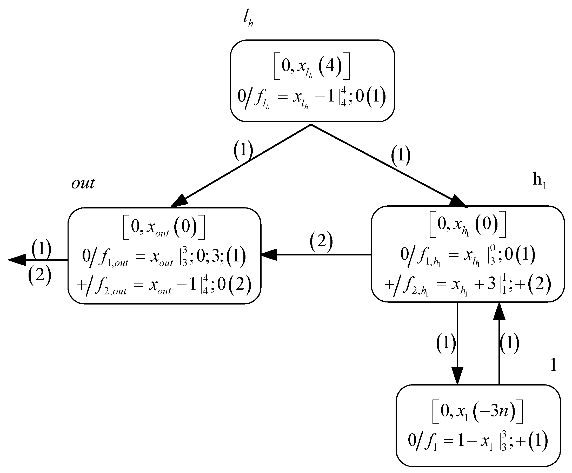
3.1.2. Module SUB—Simulating an SUB Instruction l i : ( S U B ( r ) , l j , l k )

Figure 4 displays the architecture of the SUB module and the state of the neurons it contains. Suppose system Π 1 starts to simulate the SUB instruction l i : ( S U B ( r ) , l j , l k ) at a certain time moment t = t after variable x l i of neuron σ l i has received a value of 4. Thus, production functions 0 / f 1 , i 1 = x i 1 1 | 4 1 ; 0 ; ( 1 ) and 0 / f 1 , i 1 = x i 1 1 | 4 3 ; 0 ; 1 ; ( 2 ) satisfy the application condition. Production function 0 / f 1 , i 1 = x i 1 1 | 4 1 ; 0 ( 1 ) executes first and neuron σ l i sends a value of 3 to neuron σ r , indicating that system Π 1 has completed the operation of subtracting 1 from the value stored in register r . The following two situations will occur for neuron σ r .
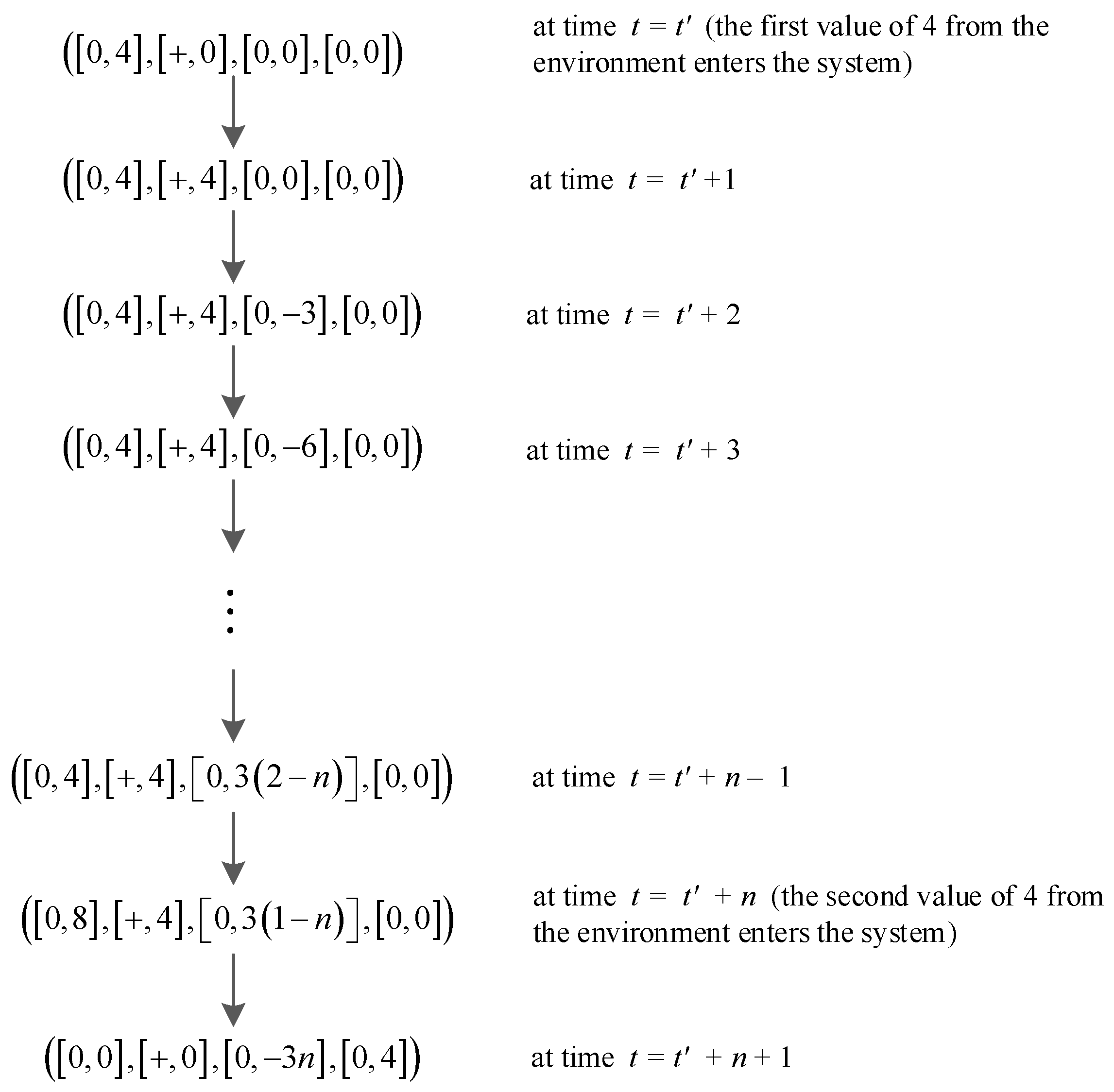
  • One situation is that the value of variable x r , i.e., the number stored in register r , is 0 at time t = t . Production function 0 / f r = x r 2 | 3 3 ; + ; ( 1 ) satisfies the threshold condition after variable x r receives a value of 3. At time t = t + 1 , with the execution of this production function, neuron σ r transmits a positive charge and a value of 1 to neurons σ i 1 and σ i 2 , respectively. Since production function 0 / f 2 , i 1 = x i 1 1 | 4 3 ; 0 ; 1 ; ( 2 ) has a postponement feature, neuron σ l i sends a value of 3 to neuron σ i 1 at time t = t + 1 . After production functions 0 / f r = x r 2 | 3 3 ; + ; ( 1 ) and 0 / f 1 , i 1 = x i 1 1 | 4 3 ; 0 ; 1 ; ( 2 ) execute, the polarization of neuron σ i 1 becomes positive, and the value of variable x i 1 becomes 4. Therefore, production function + / f 2 , i 1 = x i 1 + 3 | 4 4 ; 0 ; ( 2 ) executes at time t = t + 2 . Then, neuron σ i 1 transmits a value of 7 to neuron σ i 2 via synaptic channel ( 2 ) . Consequently, the polarization of neuron σ i 2 becomes positive and the value of variable x i 2 accumulates to 8, causing neuron σ i 2 to transmit a value of 4 to neuron σ l k . Since neuron σ l k receives a value of 4, system Π 1 starts to simulate instruction l k .
  • The other situation is that the value of variable x r is − 3 n with n N + at time t = t , i.e., the value stored in register r is greater than 0. After getting a value of 3 from neuron σ l i , the value of variable x r becomes 3 3 n , which does not satisfy the threshold condition of production function 0 / f r = x r 2 | 3 3 ; + ; ( 1 ) . Thus, neuron σ r will not fire at time t = t + 1 . However, due to the execution of production function 0 / f 1 , i 1 = x i 1 1 | 4 3 ; 0 ; 1 ; ( 2 ) , variable x i 1 receives a value of 3 from neuron σ i 1 at time t = t + 1 , causing production function 0 / f 1 , i 1 = x i 1 + 1 | 3 3 ; 0 ; ( 1 ) to execute at time t = t + 2 . Ultimately neuron σ l j receives a value of 4 from neuron σ i 1 , leading system Π 1 to start simulating instruction l j .
Consequently, the SUB module can simulate the SUB instruction l i : ( S U B ( r ) , l j , l k ) correctly. Specifically, system Π 1 is activated when variable x l i receives the value of 4, then 1 is subtracted from the value stored in register r , and finally an instruction, l j or l k , is selected non-deterministically for simulation according to the value contained in register r .

3.1.3. Module FIN—Simulating a HALT Instruction l h : H A L T

Figure 5 shows the architecture of the FIN module. At time t = t , the FIN module is activated after variable x l h receives a value of 4. This step also indicates that system Π 1 has reached the HALT instruction l h : H A L T , i.e., the simulation of register machine M has completed.
Assuming the value of variable x 1 in neuron σ 1 is 3 n with n N + at time t = t , meaning that a number n is stored in register 1. At time t = t + 1 , due to the execution of production function 0 / f l h = x l h 1 | 4 4 ; 0 ; ( 1 ) , both variables x o u t and x h 1 get a value of 3. At the next time moment t = t + 2 , both production functions 0 / f 1 , o u t = x o u t | 3 3 ; 0 ; 3 ; ( 1 ) and 0 / f 1 , h 1 = x h 1 | 3 0 ; 0 ; ( 1 ) can apply. With the execution of production function 0 / f 1 , h 1 = x h 1 | 3 0 ; 0 ; ( 1 ) , variable x 1 gets a value of 3, indicating that 1 is subtracted from the number stored in register 1. Because production function 0 / f 1 , o u t = x o u t | 3 3 ; 0 ; 3 ; ( 1 ) needs to postpone by three steps to execute, neuron σ o u t emits the first nonzero value of 3 to the environment at time t = t + 4 . Since the consumption rate of variable x h 1 is 0, i.e., the value of variable x h 1 is still 3 at time t = t + 3 , production function 0 / f 1 , h 1 = x h 1 | 3 0 ; 0 ; ( 1 ) in neuron σ h 1 can continue to execute until time t = t + n + 2 .
From time t = t + 2 to time t = t + n + 2 , variable x 1 gets a total value of 3 n + 3 . Therefore, the value of variable x 1 at time t = t + n + 2 is 3, which is equal to the threshold of production function 0 / f 1 = 1 x 1 | 3 3 ; + ; ( 1 ) . With the execution of production function 0 / f 1 = 1 x 1 | 3 3 ; + ; ( 1 ) , a value of 2 and a positive charge are transmitted to neuron σ h 1 . Thus, production function + / f 2 , h 1 = x h 1 + 3 | 1 1 ; + ; ( 1 ) is activated at time t = t + n + 3 . Since the polarization of neuron σ o u t becomes positive and variable x o u t gets a value of 4, production function 0 / f 2 , o u t = x o u t 1 | 4 4 ; 0 ; ( 2 ) executes and neuron σ o u t emits the second nonzero value of 3 into the environment via synaptic channel ( 2 ) at time t = t + n + 4 . Production function 0 / f 1 = 1 x 1 | 3 3 ; + ; ( 1 ) in neuron σ 1 can also execute at time t = t + n + 3 , leading the value of variable x h 1 to become −2. At this point, the system runs to the final configuration because the values of the variables in the neurons no longer satisfy the conditions for the production functions to execute.
From the above discussions, the time interval between the two firings of the output neuron is ( t + n + 4 ) ( t + 4 ) = n , which is exactly the same as the number stored in register 1. As specified in the definition, the computation result of system Π 1 is equal to n .
Through the discussions of the operating mechanism of the ADD, SUB, and FIN modules, system Π 1 is verified to simulate register machine M correctly in its generating mode, i.e., N 2 ( Π 1 ) = N ( M ) . In addition, system Π 1 uses only two types of, i.e., neutral and positive, polarizations, and all production functions are linear with at most one variable. Accordingly, N 2 c h 2 N S N V C   P ( p o l y 1 ( 1 ) ) = N R E holds.

3.2. NSNVC P Systems as Number Accepting Devices

When used as a number accepting device, a NSNVC P system Π can accept a number n . In this situation, the function of the input neuron σ i n is to accept values from the external environment. Initially, the number n to be computed is accepted by system Π in the form 40 n 1 4 , where 4 and 0 are the values introduced into the system. Specifically, assuming that input variable x i n receives a value of 4 at time t = t 1 and t = t 2 respectively, the time interval between t = t 1 and t = t 2 , i.e., n = t 2 t 1 is defined as the number accepted by system Π . Afterwards, the number n is processed by a series of instructions. When it runs to the final configuration, system Π is considered to have accepted the number n .
Theorem 2.
N a c c c h 2 N S N V C   P ( p o l y 1 ( 1 ) ) = N R E .
Proof. 
The proof of the inclusion N R E N a c c c h 2 N S N V C   P ( p o l y 1 ( 1 ) ) is verified by simulating deterministic register machines working in the accepting mode, while the converse inclusion is directly confirmed by the Turing-Church thesis [41]. □
The form of a deterministic register machine is M = ( m ¯ , H , l 0 , l h , I ) . Each element of M has the same meaning as that of the corresponding element of the non-deterministic register machine M working in the generating mode. The only difference between M and M is in the form of the ADD instructions. The ADD instructions in M are defined as a deterministic form l i : ( A D D ( r ) , l j ) . In addition, the set consisting of all the numbers accepted by M is represented by N acc ( M ) .
A NSNVC P system Π 2 is designed to simulate machine M with a similar structure to that of system Π 1 in the generating mode. Especially, system Π 2 consists of a deterministic ADD module, a SUB module, and an INPUT module. The INPUT module is used to introduce numbers to be processed into system Π 2 . The functions of the other two modules remain the same as those in system Π 1 .
The architecture of the INPUT module is shown in Figure 6. In the initial configuration, the values of all the variables in system Π 2 are 0. The input variable x i n is assumed to have a value of 4 at time t = t , so that production function 0 / f 1 , i n = x i n | 4 0 ; + ; ( 1 ) satisfies the execution condition. Consequently, neuron σ i n sends a positive charge and a value of 4 to neuron σ i n 1 via synaptic channel ( 1 ) . Because the consumption rate of variable x i n is 0, the value of variable x i n is still 4 at time t = t + 1 . Therefore, production function 0 / f 1 , i n = x i n | 4 0 ; + ; ( 1 ) will continue to execute at each subsequent time moment until variable x i n again has a value of 4.
At time t = t + 1 , neuron σ i n 1 executes production function + / f i n 1 = 1 x i n 1 | 4 4 ; 0 ; ( 1 ) and transmits a value of −3 to neuron σ 1 , simulating the addition of 1 to the number stored in register 1. Simultaneously, variable x i n 1 receives a value of 4 from neuron σ i n . Accordingly, neuron σ i n 1 will send a value of −3 to neuron σ 1 at time t = t + 2 again. In fact, neuron σ 1 receives a value of −3 at every step from time t = t + 2 to time t = t + n + 1 . Thus, variable x 1 gets a total value of 3 n , i.e., register 1 stores the number n .
At time t = t + n , the value of variable x i n becomes 8 because it receives another value of 4 from the external environment. In this way, production function + / f 2 , i n = 1 2 x i n | 8 8 ; 0 ; ( 2 ) of neuron σ i n can execute. Consequently, neuron σ i n sends a value of 4 to neuron σ l 0 via synaptic channel ( 2 ) , indicating that system Π 2 is about to simulate instruction l 0 of machine M .
The configuration dynamics of the INPUT module is shown in Figure 7. The configuration at each time moment involves variables x i n , x i n 1 , x 1 and x l 0 in that order.
The deterministic ADD module, illustrated in Figure 8, is used to simulate a deterministic ADD instruction l i : ( A D D ( r ) , l j ) . The simulation starts when neuron σ l i receives a value of 4. Suppose that neuron σ l i receives a value of 4 at time t = t , then production function + / f 1 , l i = x l i | 4 1 ; 0 ; ( 1 ) executes and neuron σ l i sends a value of 4 to neuron σ l j via synaptic channel ( 1 ) . Since the consumption rate of variable x l i is 1, production function + / f 2 , l i = x l i | 3 3 ; 0 ; ( 2 ) meets the application conditions. Consequently, register r receives a value of 3 at time t = t + 2 . So far, system Π 2 has completed the simulation of instruction l i and finished the operation of adding 1 to the number stored in register r .
Moreover, the SUB module in system Π 2 is exactly the same as that in system Π 1 . System Π 2 does not have a FIN module, but has neuron σ l h . System Π 2 has completed the simulation of M if variable x l h in neuron σ l h gets a value of 4 at any point of time. At this time point, system Π 2 has reached the HALT instruction and has accepted the number n .
The above discussions show that system Π 2 working in the accepting mode can successfully simulate M , i.e., N a c c ( Π 2 ) = N a c c ( M ) . In addition, the structures of the three modules show that all the production functions are linear each with at most one variable and the neurons have only two types of, i.e., neutral and positive, polarizations in system Π 2 . Consequently, N a c c c h 2 N S N V C   P ( p o l y 1 ( 1 ) )   =   N R E holds.

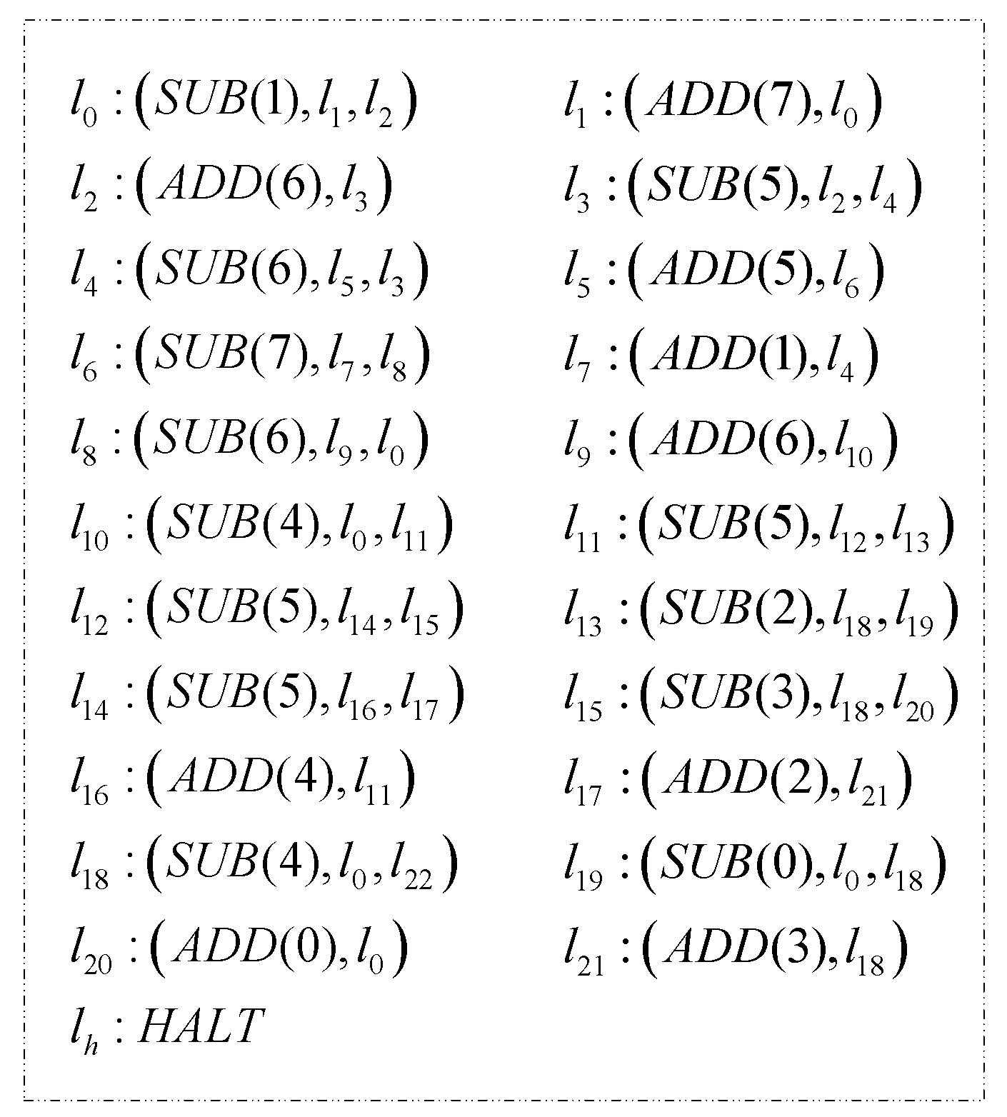
4. Turing Universality of NSNVC P Systems for Computing Functions

The lower limit on the number of neurons needed in a NSNVC P system as a universal function computing device is discussed in this section. In order to compute function f : N k N , a register machine M c = ( m ˙ ¯ , H , l 0 , l h , I ) works as follows. First, generally registers 1 to k of machine M c store the values of the k arguments, and all other registers are empty. Then, machine M c starts a computation by executing the instruction labeled l 0 , and executes a series of instructions to continue the computation. Finally, the value of function f computed by M c is stored in another specific register r t when the HALT instruction l h is reached. Assume ( φ 0 , φ 1 , ) is a fixed admissible enumeration of a unary partially recursive function. If a recursive function f satisfies φ X ( y ) = M u ( f ( x ) , y ) for natural numbers x and y , then the register machine is considered universal.
Korec [45] introduced a small universal register machine M u = ( 8 , H , l 0 , l h , I ) for function computing, as illustrated in Figure 9. The register machine M u consists of 23 instructions and 8 registers numbered from 0 to 7. Initially, two arguments f ( x ) and y are introduced into registers 1 and 2, respectively, which enable machine M u to compute any φ x ( y ) . Moreover, when the computation of M u halts, the number stored in register 0 is the computation result of function φ x ( y ) . A NSNVC P system is designed to simulate machine M u . For this purpose, M u is modified as follows. A new register 8 is added, and the original HALT instruction is replaced by three instructions l 22 : ( S U B ( 0 ) , l 23 , l h ) , l 23 : ( A D D ( 8 ) , l 22 ) and l h : H A L T . In this way, the calculation result is stored in register 8. The modified register machine is represented by M u , which consists of 9 registers, labeled from 0 to 8, and 25 instructions, including 14 SUB instructions, 10 ADD instructions and 1 HALT instruction.
Theorem 3.
There is a Turing universal NSNVC P System with 66 neurons to be used as a function computing device.
Proof. 
A NSNVC P system Π 3 is designed to simulate the computation functions of register machine M u . System Π 3 is composed of an INPUT module, an OUTPUT module, 10 ADD modules, and 14 SUB modules. The ADD modules adopt a deterministic form. Assume that the values of all the variables in system Π 3 are 0 initially. A correspondence exists between the elements, i.e., the registers and instructions, of M u and the elements, i.e., the neurons, of system Π 3 . □
The INPUT module of system Π 3 is shown in Figure 10. The function of this module is to introduce two natural numbers 3 f ( x ) and 3 y into neurons σ 1 and σ 2 , respectively, through the sequence in the form 40 f ( x ) 1 40 y 1 4 , where 4 and 0 are the values introduced into the system. The configuration dynamics of the INPUT module is shown in Figure 11. Each configuration involves neurons σ i n , σ i n 1 , σ i n 2 , σ 1 , σ 2 and σ l 0 in that order.
The input neuron σ i n is used to read the sequence 40 f ( x ) 1 40 y 1 4 . Assuming that input variable x i n gets a value of 4 at time t = t 1 , then production function 0 / f 1 , i n = x i n | 4 0 ; + ; ( 1 ) executes and neuron σ i n transmits a positive charge and a value of 4 to neuron σ i n 1 . At time t = t 1 + 1 , production function + / f i n 1 = 1 x i n 1 | 4 4 ; 0 ; ( 1 ) in neuron σ i n 1 satisfies the execution condition and neuron σ i n 1 sends a value of −3 to neuron σ 1 . As a result, the value stored in neuron σ 1 increases by 1. In addition, since the value of variable x i n will not be consumed after production function 0 / f 1 , i n = x i n | 4 0 ; + ; ( 1 ) executes, neuron σ i n sends the value of 4 to neuron σ i n 1 at each time moment after time t = t 1 . This process continues until neuron σ i n receives a value of 4 again. Therefore, from time t = t 1 + 2 to time t = t 1 + f ( x ) + 1 , neuron σ 1 receives a total value of 3 f ( x ) from neuron σ i n 1 , i.e., the number stored in register 1 is f ( x ) .
Suppose the input neuron σ i n receives a value of 4 again and the value of variable x i n accumulates to 8 at time t = t 2 , (in fact, t 2 = t 1 + f ( x ) ). Production function 0 / f 2 , i n = 1 2 x i n | 8 0 ; + ; ( 2 ) executes and neuron σ i n sends a value of 4 to neuron σ i n 2 via synaptic channel ( 2 ) . At time t = t 2 + 1 , with the execution of production function + / f i n 2 = 1 x i n 2 | 4 4 ; 0 ; ( 1 ) , neuron σ i n 2 sends a value of −3 to neuron σ 2 for the first time. Similarly, because the accumulated value received by neuron σ 2 from neuron σ i n 2 is 3 y from time t = t 2 + 2 to time t = t 2 + y + 1 , the number stored in register 2 is y .
The value of variable x i n becomes 12 after neuron σ i n receives the value of 4 for the third time at time t = t 3 , (in fact, t 3 = t 2 + y ). When production function 0 / f 3 , i n = 1 3 x i n | 12 12 ; 0 ; ( 3 ) executes, variable x l 0 gets a value of 4, causing system Π 3 to start the simulation of the initial instruction l 0 .
Thereafter, no production function can be applied and system Π 3 starts to use the ADD and SUB modules to simulate machine M u . All the ADD instructions in machine M u are of the form l i : ( A D D ( r ) , l j ) as shown in Figure 9. Therefore, the deterministic ADD module in the number accepting device system Π 2 , as shown in Figure 8, can be used to simulate these instructions. Moreover, the SUB module shown in Figure 4 is used to simulate the SUB instructions l i : ( S U B ( r ) , l j , l k ) . Hence, the discussions of the ADD and SUB modules are not repeated. The OUTPUT module is constructed by modifying the FIN module shown in Figure 4. Specifically, neuron σ 1 in the FIN module shown in Figure 4 is replaced by neuron σ 8 in the OUTPUT module. The process of NSNVC P system Π 3 simulating register machine M u is illustrated in Figure 12.
Through the above discussion, NSNVC P system Π 3 can correctly simulate register machine M u . The system contains 66 neurons in total, and has the following details for the neurons:
  • 25 neurons associated with 25 instruction labels;
  • 9 neurons associated with 9 registers;
  • 2 × 14 auxiliary neurons for 14 SUB modules;
  • 3 neurons in the INPUT module;
  • 2 neurons in the OUTPUT module.
In fact, some optimization techniques such as combining some consecutive ADD and/or SUB instructions can further decrease the number of neurons. Neuron σ 21 in system Π 3 can be omitted by combining consecutive instructions l 17 : ( A D D ( 2 ) , l 21 ) and l 21 : ( A D D ( 3 ) , l 18 ) . The combined instructions can be simulated with the ADD-ADD module shown in Figure 13. Because the value required to start the simulation of an instruction is inconsistent with the value required for a register to add or subtract 1, the combined ADD and/or SUB instructions will not be further discussed in this work. Therefore, a universal NSNVC P system requiring only 66 neurons is obtained as a function computing device.
Compared with NSN P systems, each module of NSNVC P systems needs fewer neurons, indicating that a series of improvements to NSN P systems are successful. These improvements include the proposed variable consumption strategy, the use of polarization and threshold as two conditions to control the execution of production functions, the postponement feature assigned to production functions and the introduction of multiple synaptic channels.
Some of the latest computing models [17,42,43,44] and a classic computing model [13] as function computing devices are listed in Table 2 along with their numbers of computing units, i.e., neurons. As shown in Table 2, NSNVC P systems need fewer neurons than SNP-IR systems [42], PASN P systems [43], PSNRS P systems [44], and DTNP systems [13] to obtain Turing universality as function computing devices. Although SNP-MC systems [17] need only 38 neurons, fewer than that of NSNVC P systems, to obtain Turing universality as function computing devices, they are in the type of discrete computing models due to the use of spiking rules. However, NSNVC P systems are in the type of continuous computing models with numerical attributes and are more suitable for solving practical problems due to the use of production functions instead of spiking rules. The comparison in Table 2 shows the computational power of NSNVC P systems. Apparently, NSNVC P systems have better computing capability and performance than most other P systems.

5. Conclusions

A new variant of NSN P systems, called NSNVC P systems, is proposed by improving the NSN P systems. The improvements are the proposed variable consumption strategy, the use of polarization and threshold, the postponement features of the production functions, and the use of multiple synaptic channels. By simulating register machines, the computational completeness of NSNVC P systems as number generating/accepting devices is proved. Furthermore, a universal NSNVC P system with 66 neurons is constructed to compute Turing computable functions.
The new variable consumption strategy makes NSNVC P systems more flexible and practical. Different from NSN P systems, each production function in NSNVC P systems is assigned a threshold and a polarization. A production function must simultaneously satisfy the threshold and polarization conditions to execute. It is precisely because of these two conditions, NSNVC P systems achieved Turing universality by using only positive and neutral polarizations. These two conditions do not inhibit the operation, but complement each other and enhance the controlling ability, of NSNVC P systems.
The introduction of multiple synaptic channels has contributed to the flexibility of operations of NSNVC P systems. This is particularly evident in the INPUT module shown in Figure 9. The postponement feature assigned to production functions also plays an important role in NSNVC P systems. For example, if production function 0 / f 1 , o u t = x o u t | 3 3 ; 0 ; 3 ; ( 1 ) of neuron σ o u t in the FIN module does not have the postponement feature, neuron σ o u t will need more production functions, or the FIN module will need more neurons, to achieve the same result.
The universality of NSNVC P systems is studied in this work, and further works are needed to use NSNVC P systems to solve some specific real-world problems. By introducing polarizations, multiple synaptic channels, the variable consumption strategy and the postponement feature, the dimension of the coded information in NSNVC P systems increases. Therefore, NSNVC P systems are more suitable for solving practical problems, such as image processing, fault diagnosis, and robots, which requires more ways for information representation.

Author Contributions

Conceptualization, X.Y. and M.S.; methodology, X.Y.; formal analysis, X.Y.; writing—original draft preparation, X.Y.; writing—review and editing, X.Y. and M.S.; visualization, X.Y.; supervision, M.S., X.L., and Q.R.; funding acquisition, X.L. All authors have read and agreed to the published version of the manuscript.

Funding

This research project was funded by the National Natural Science Foundation of China (61876101, 61802234, 61806114), Social Science Fund Project of Shandong Province, China (16BGLJ06, 11CGLJ22), Natural Science Fund Project of Shandong Province, China (ZR2019QF007), Postdoctoral Project, China (2017M612339, 2018M642695), Humanities and Social Sciences Youth Fund of the Ministry of Education, China (19YJCZH244), and Postdoctoral Special Funding Project, China (2019T120607).

Conflicts of Interest

The authors declare no conflict of interest.

References

  1. Păun, G. Computing with membranes. J. Comput. Syst. Sci. 2000, 61, 108–143. [Google Scholar] [CrossRef] [Green Version]
  2. Song, T.; Gong, F.; Liu, X. Spiking neural P systems with white hole neurons. IEEE Trans. NanoBiosci. 2016, 15, 666–673. [Google Scholar] [CrossRef] [PubMed]
  3. Ionescu, M.; Păun, G.; Yokomori, T. Spiking neural P systems. Fund. Inform. 2006, 71, 279–308. [Google Scholar]
  4. Păun, G. Spiking neural P systems with astrocyte-like control. J. UCS 2007, 13, 1707–1721. [Google Scholar]
  5. Pan, L.; Wang, J.; Hoogeboom, H. Spiking neural P systems with astrocytes. Neural Comput. 2012, 24, 805–825. [Google Scholar] [CrossRef] [PubMed]
  6. Pan, L.; Păun, G. Spiking neural P systems with anti-spikes. Int. J. Comput. Commun. Control 2009, 4, 273–282. [Google Scholar] [CrossRef] [Green Version]
  7. Wu, T.; Păun, A.; Zhang, Z.; Pan, L. Spiking neural P systems with polarizations. IEEE Trans. Neural Netw. Learn. Syst. 2018, 29, 3349–3360. [Google Scholar]
  8. Song, T.; Pan, L.; Păun, G. Spiking neural P systems with rules on synapses. Theoret. Comput. Sci. 2014, 529, 82–95. [Google Scholar] [CrossRef]
  9. Peng, H.; Yang, J.; Wang, J.; Wang, T.; Sun, Z.; Song, X.; Luo, X.; Huang, X. Spiking neural P systems with multiple channels. Neural Netw. 2017, 95, 66–71. [Google Scholar] [CrossRef]
  10. Song, X.; Wang, J.; Peng, H.; Ning, G.; Sun, Z.; Wang, T.; Yang, F. Spiking neural P systems with multiple channels and anti-spikes. Biosystems 2018, 169, 13–19. [Google Scholar] [CrossRef]
  11. Wang, J.; Hoogeboom, H.; Pan, L.; Păun, G.; Pérez-Jiménez, M. Spiking neural P systems with weights. Neural Comput. 2010, 22, 2615–2646. [Google Scholar] [CrossRef] [PubMed]
  12. Zeng, X.; Zhang, X.; Song, T.; Pan, L. Spiking neural P systems with thresholds. Neural Comput. 2014, 26, 1340–1361. [Google Scholar] [CrossRef]
  13. Peng, H.; Wang, J.; Pérez-Jiménez, M.J.; Riscos-Núñez, A. Dynamic threshold neural P systems. Knowl. Based Syst. 2019, 163, 875–884. [Google Scholar] [CrossRef]
  14. Peng, H.; Wang, J. Coupled Neural P Systems. IEEE Trans. Neural Netw. Learn. Syst. 2019, 30, 1672–1682. [Google Scholar] [CrossRef]
  15. Cavaliere, M.; Ibarra, O.H.; Păun, G.; Egecioglu, O.; Ionescu, M.; Woodworth, S. Asynchronous spiking neural P systems. Theor. Comput. Sci. 2009, 410, 2352–2364. [Google Scholar] [CrossRef] [Green Version]
  16. Song, T.; Pan, L.; Păun, G. Asynchronous spiking neural P systems with local synchronization. Inf. Sci. 2013, 219, 197–207. [Google Scholar] [CrossRef] [Green Version]
  17. Song, X.; Peng, H.; Wang, J.; Ning, G.; Sun, Z. Small universal asynchronous spiking neural P systems with multiple channels. Neurocomputing 2020, 378, 1–8. [Google Scholar] [CrossRef]
  18. Cabarle, F.G.C.; Adorna, H.N.; Jiang, M.; Zeng, X. Spiking neural P systems with scheduled synapses. IEEE Trans. Nanobiosci. 2017, 16, 792–801. [Google Scholar] [CrossRef] [PubMed]
  19. Pan, L.; Păun, G.; Zhang, G.; Neri, F. Spiking neural P systems with communication on request. Int. J. Neural Syst. 2017, 27, 1750042. [Google Scholar] [CrossRef] [Green Version]
  20. Yin, X.; Liu, X. Dynamic Threshold Neural P Systems with Multiple Channels and Inhibitory Rules. Processes 2020, 8, 1281. [Google Scholar] [CrossRef]
  21. Kong, Y.; Zheng, Z.; Liu, Y. On string languages generated by spiking neural P systems with astrocytes. Fundam. Inform. 2015, 136, 231–240. [Google Scholar] [CrossRef]
  22. Zhang, X.; Zeng, X.; Pan, L. On string languages generated by spiking neural P systems with exhaustive use of rules. Nat. Comput. 2008, 7, 535–549. [Google Scholar] [CrossRef]
  23. Cabarle, F.; Adorna, H.; Pérez-Jiménez, M.; Song, T. Spiking neuron P systems with structural plasticity. Neural Comput. Appl. 2015, 26, 1905–1917. [Google Scholar] [CrossRef]
  24. Peng, H.; Chen, R.; Wang, J.; Song, X.; Wang, T.; Yang, F.; Sun, Z. Competitive spiking neural P systems with rules on synapses. IEEE Trans. NanoBiosci. 2017, 16, 888–895. [Google Scholar] [CrossRef]
  25. Ren, Q.; Liu, X.; Sun, M. Turing Universality of Weighted Spiking Neural P Systems with Anti-spikes. Comput. Intell. Neurosci. 2020, 2020, 1–10. [Google Scholar] [CrossRef]
  26. Păun, G.; Păun, R. Membrane computing and economics: Numerical P systems. Fundam. Inform. 2006, 73, 213–227. [Google Scholar]
  27. Zhang, Z.; Su, Y.; Pan, L. The computational power of enzymatic numerical P systems working in the sequential mode. Theor. Comput. Sci. 2018, 724, 3–12. [Google Scholar] [CrossRef]
  28. Pan, L.; Zhang, Z.; Wu, T.; Xu, J. Numerical P systems with production thresholds. Theor. Comput. Sci. 2017, 673, 30–41. [Google Scholar] [CrossRef]
  29. Liu, L.; Yi, W.; Yang, Q.; Peng, H.; Wang, J. Numerical P systems with Boolean condition. Theor. Comput. Sci. 2019, 785, 140–149. [Google Scholar] [CrossRef]
  30. Díaz-Pernil, D.; Peña-Cantillana, F.; Gutiérrez-Naranjo, M.A. A parallel algorithm for skeletonizing images by using spiking neural P systems. Neurocomputing 2013, 115, 81–91. [Google Scholar] [CrossRef]
  31. Xiang, M.; Dan, S.; Ashfaq, K. Image Segmentation and Classification Based on a 2D Distributed Hidden Markov Model. Proc. Int. Soc. Opt. Eng. 2008, 6822, 51. [Google Scholar]
  32. Zhang, G.; Gheorghe, M.; Li, Y. A membrane algorithm with quantum-inspired subalgorithms and its application to image processing. Natural Comput. 2012, 11, 701–717. [Google Scholar] [CrossRef]
  33. Buiu, C.; Vasile, C.; Arsene, O. Development of membrane controllers for mobile robots. Inf. Sci. 2012, 187, 33–51. [Google Scholar] [CrossRef]
  34. Wang, X.; Zhang, G. Design and implementation of membrane controllers for trajectory tracking of nonholonomic wheeled mobile robots. Integr. Comput. Aided Eng. 2016, 23, 15–30. [Google Scholar] [CrossRef] [Green Version]
  35. Xiong, G.; Shi, D.; Zhu, L.; Duan, X. A new approach to fault diagnosis of power systems using fuzzy reasoning spiking neural P systems. Math. Probl. Eng. 2013, 2013, 211–244. [Google Scholar] [CrossRef] [Green Version]
  36. Wang, T.; Zhang, G.; Zhao, J.; He, Z.; Wang, J.; Pérez-Jiménez, M.J. Fault diagnosis of electric power systems based on fuzzy reasoning spiking neural P systems. IEEE Trans. Power Syst. 2014, 30, 1182–1194. [Google Scholar] [CrossRef]
  37. Peng, H.; Wang, J.; Ming, J.; Shi, P.; Pérez-Jiménez, M.J.; Yu, W.; Tao, C. Fault diagnosis of power systems using intuitionistic fuzzy spiking neural P systems. IEEE Trans. Smart Grid. 2018, 9, 4777–4784. [Google Scholar] [CrossRef]
  38. Peng, H.; Wang, J.; Shi, P.; Pérez-Jiménez, M.J.; Riscos-Núñez, A. An extended membrane system with active membrane to solve automatic fuzzy clustering problems. Int. J. Neural Syst. 2015, 26, 1650004. [Google Scholar] [CrossRef] [PubMed]
  39. Peng, H.; Shi, P.; Wang, J.; Riscos-Núñez, A.; Pérez-Jiménez, M.J. Multiobjective fuzzy clustering approach based on tissue-like membrane systems. Knowl. Based Syst. 2017, 125, 74–82. [Google Scholar] [CrossRef]
  40. Han, L.; Xiang, L.; Liu, X.; Luan, J. The K-medoids Algorithm with Initial Centers Optimized Based on a P System. J. Inf. Comput. Sci. 2014, 11, 1765–1774. [Google Scholar] [CrossRef]
  41. Wu, T.; Pan, L.; Yu, Q.; Tan, K.C. Numerical Spiking Neural P Systems. IEEE Transact. Neural Netw. Learn. Syst. 2020, 1–15. [Google Scholar] [CrossRef]
  42. Peng, H.; Li, B.; Wang, J. Spiking neural P systems with inhibitory rules. Knowl. Based Syst. 2020, 188, 105064. [Google Scholar] [CrossRef]
  43. Wu, T.; Zhang, T.; Xu, F. Simplified and yet Turing universal spiking neural P systems with polarizations optimized by anti-spikes. Neurocomputing 2020, 414, 255–266. [Google Scholar] [CrossRef]
  44. Jiang, S.; Fan, J.; Liu, Y.; Wang, Y.; Xu, F. Spiking Neural P Systems with Polarizations and Rules on Synapses. Complexity 2020, 2020, 1–12. [Google Scholar] [CrossRef]
  45. Korec, I. Small universal register machines. Theor. Comput. Sci. 1996, 168, 267–301. [Google Scholar] [CrossRef] [Green Version]
Figure 1. An example NSNVC P system Π e x .
Processes 09 00549 g001
Figure 2. Configuration dynamics of system Π e x .
Processes 09 00549 g002
Figure 3. The ADD module in system Π 1 .
Processes 09 00549 g003
Figure 4. The SUB module in system Π 1 .
Processes 09 00549 g004
Figure 5. The FIN module in system Π 1 .
Processes 09 00549 g005
Figure 6. The INPUT module in system Π 2 .
Processes 09 00549 g006
Figure 7. Configuration dynamics of the INPUT module.
Processes 09 00549 g007
Figure 8. The deterministic ADD module in system Π 2 .
Processes 09 00549 g008
Figure 9. The universal register machine M u .
Processes 09 00549 g009
Figure 10. The INPUT module in system Π 3 .
Processes 09 00549 g010
Figure 11. Configuration dynamics of the INPUT module in system Π 3 .
Processes 09 00549 g011
Figure 12. An illustration of using NSNVC P system Π 3 to simulate M u .
Processes 09 00549 g012
Figure 13. The ADD-ADD model simulating consecutive ADD-ADD instructions l 17 : ( A D D ( 2 ) , l 21 ) and l 21 : ( A D D ( 3 ) , l 18 ) .
Processes 09 00549 g013
Table 1. Abbreviations and corresponding full names of some P systems cited in this work.
SystemFull Name
SNP systems [3]Spiking neural P systems
PSN P systems [7]Spiking neural P systems with polarizations
SNP-MC systems [17]Small universal asynchronous spiking neural P systems with multiple channels
NP systems [37]Numerical P systems
NSN P systems [41]Numerical spiking neural P systems
SNP-IR systems [42]Spiking neural P systems with inhibitory rules
PASN P systems [43]Simplified and yet Turing universal spiking neural P systems with polarizations optimized by anti-spikes
PSNRS P systems [44]Spiking neural P systems with polarizations and rules on synapses
Table 2. Comparison of different computing models in the number of neurons.
Computing ModelsNumber of Neurons
NSNVC P systems66
SNP-IR systems [43]100
PASN P systems [44]121
PSNRS P systems [45]151
SNP-MC systems [17]38
DTNP systems [13]109
Publisher’s Note: MDPI stays neutral with regard to jurisdictional claims in published maps and institutional affiliations.

