
Indirect Monitoring of Anaerobic Digestion for Cheese Whey Treatment

 and
and
Abstract
:
1. Introduction
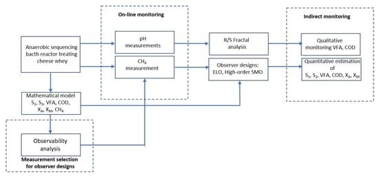
2. Materials and Methods
2.1. Experimental Set-Up for Cheese Whey Treatment
2.2. Mathematical Model for Cheese Whey Treatment
2.3. Observability Analysis
2.3.1. Linear Observability Analysis
- Kalman range condition.
- 2.
- Popov–Belevitch–Hautus (PBH) test.
- Rank condition using Lie derivatives.
- 2.
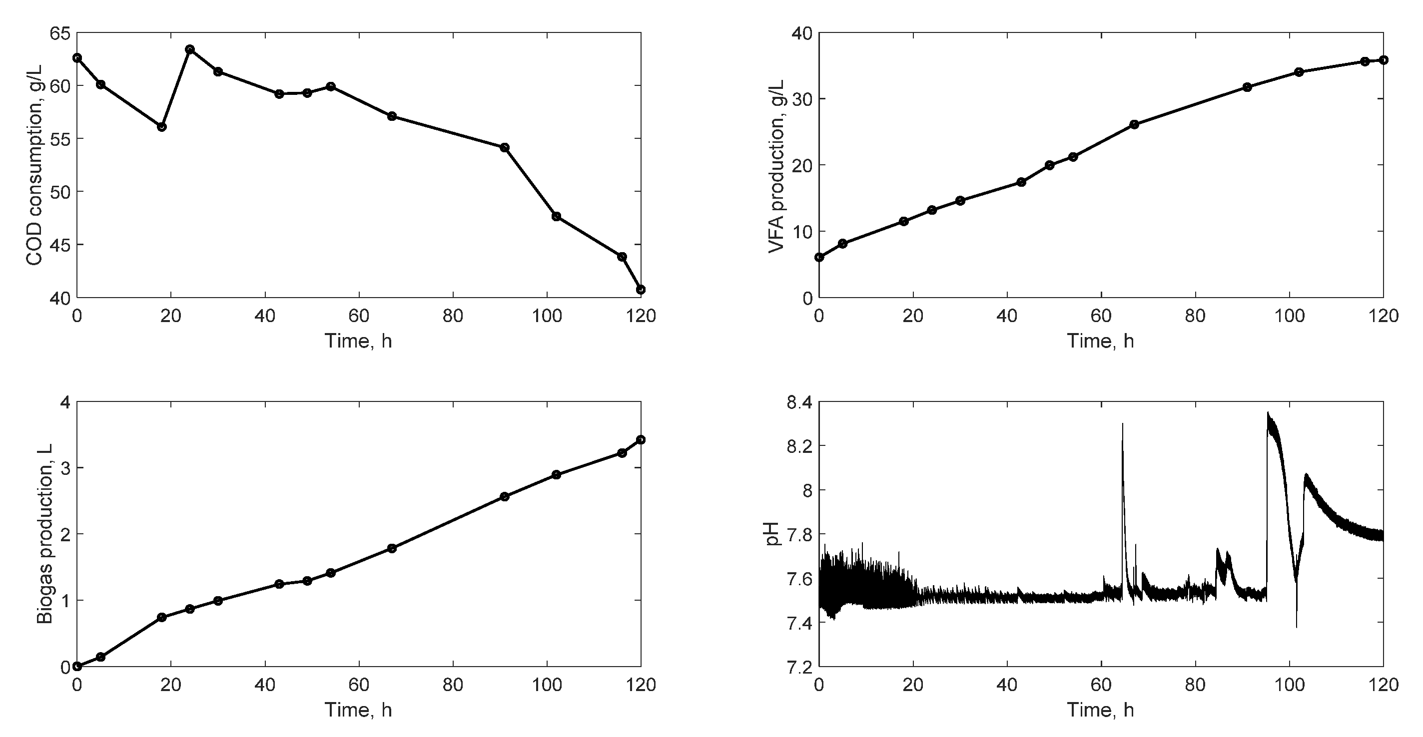
- Incidence diagrams.
- A link is drawn, xi → xj, if xj appears in the differential equation of xi. This implies that one can collect information from xj by monitoring xi as a function of time;
- The inference diagram is broken down into sets of firmly connected maximum components (SCCs), which are select graphs that directly link to each node of another sub-graph. Usually, they are enclosed in dotted circles;
- At least one node is selected from each root of the SCCs, which do not have input axes, to ensure system observability.
2.3.2. Observability Index
2.4. Observer Designs
2.4.1. Extended Luenberger Observer
2.4.2. Sliding Mode Observers
2.5. Fractal Analysis
3. Results and Discussion
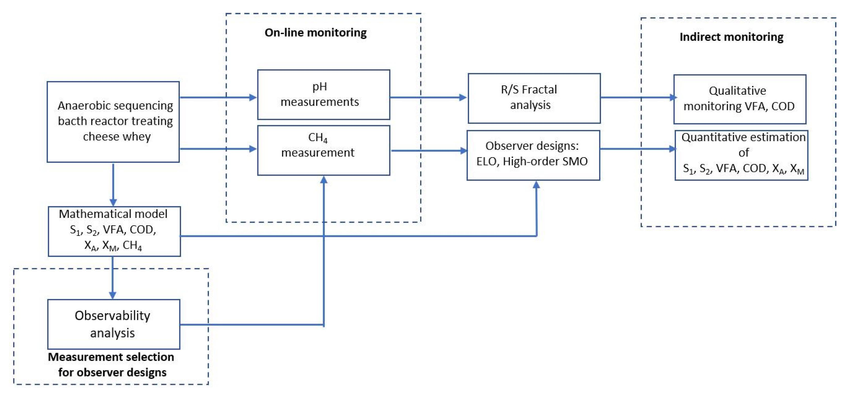
3.1. Experimental Profiles
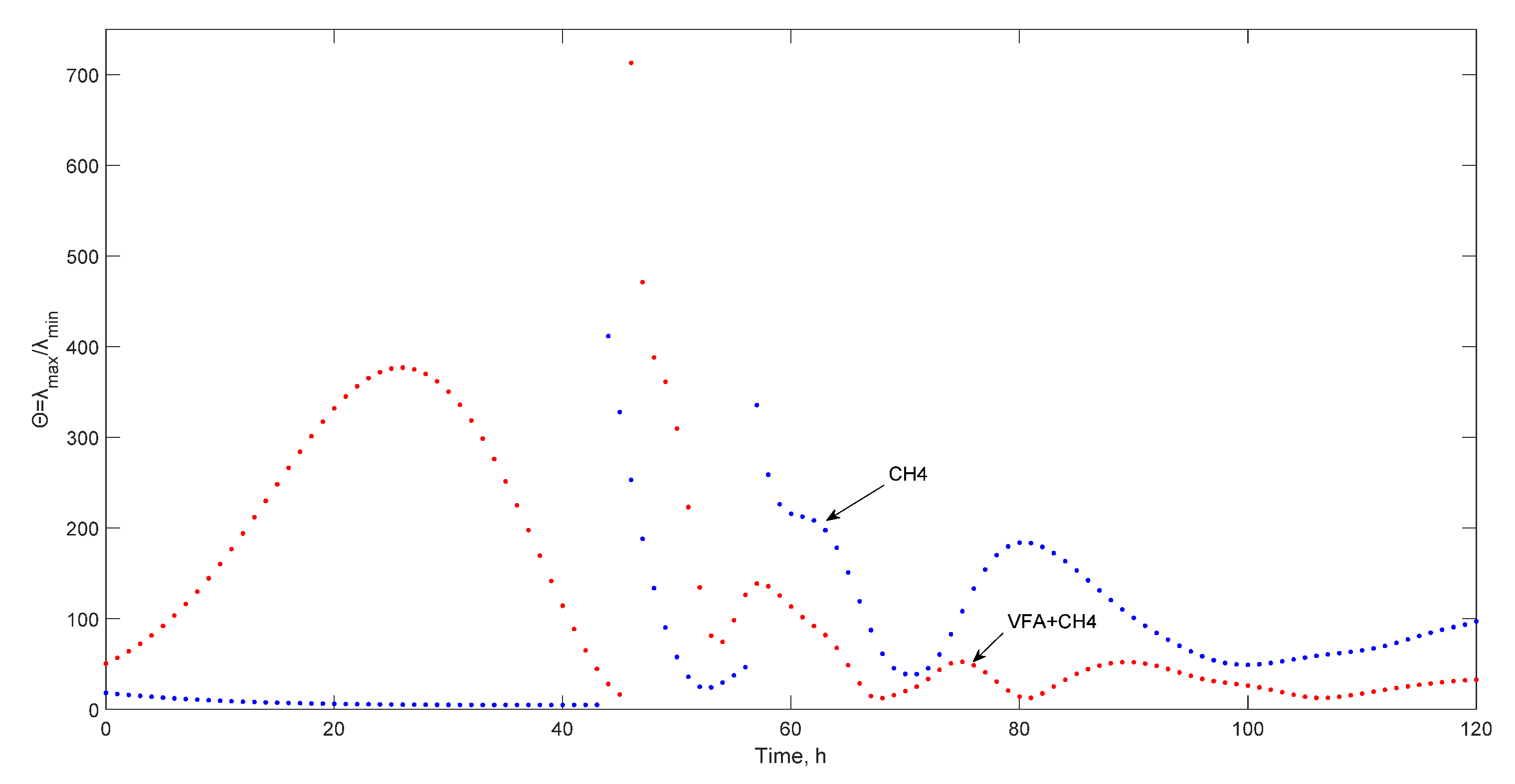
3.2. Observability Analysis
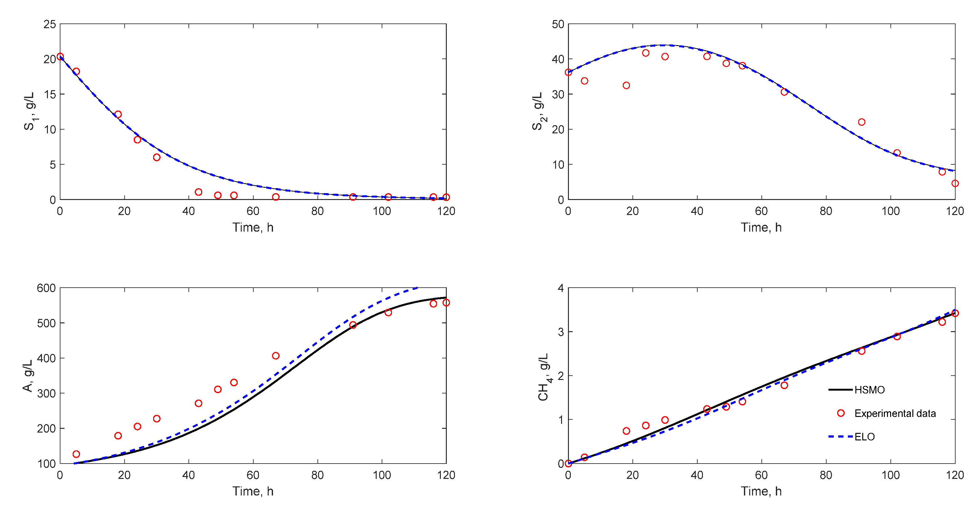
3.3. Observer Designs
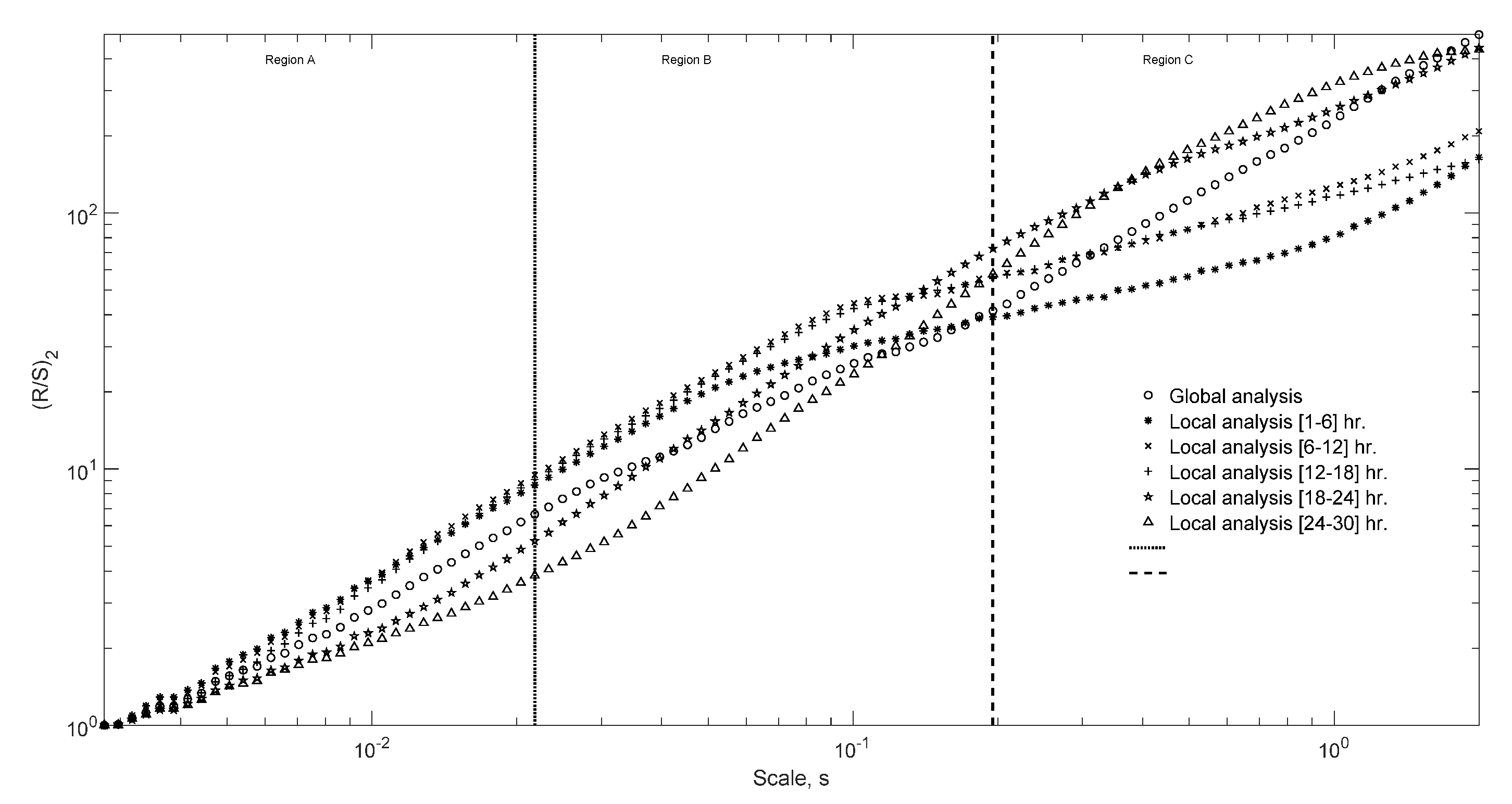
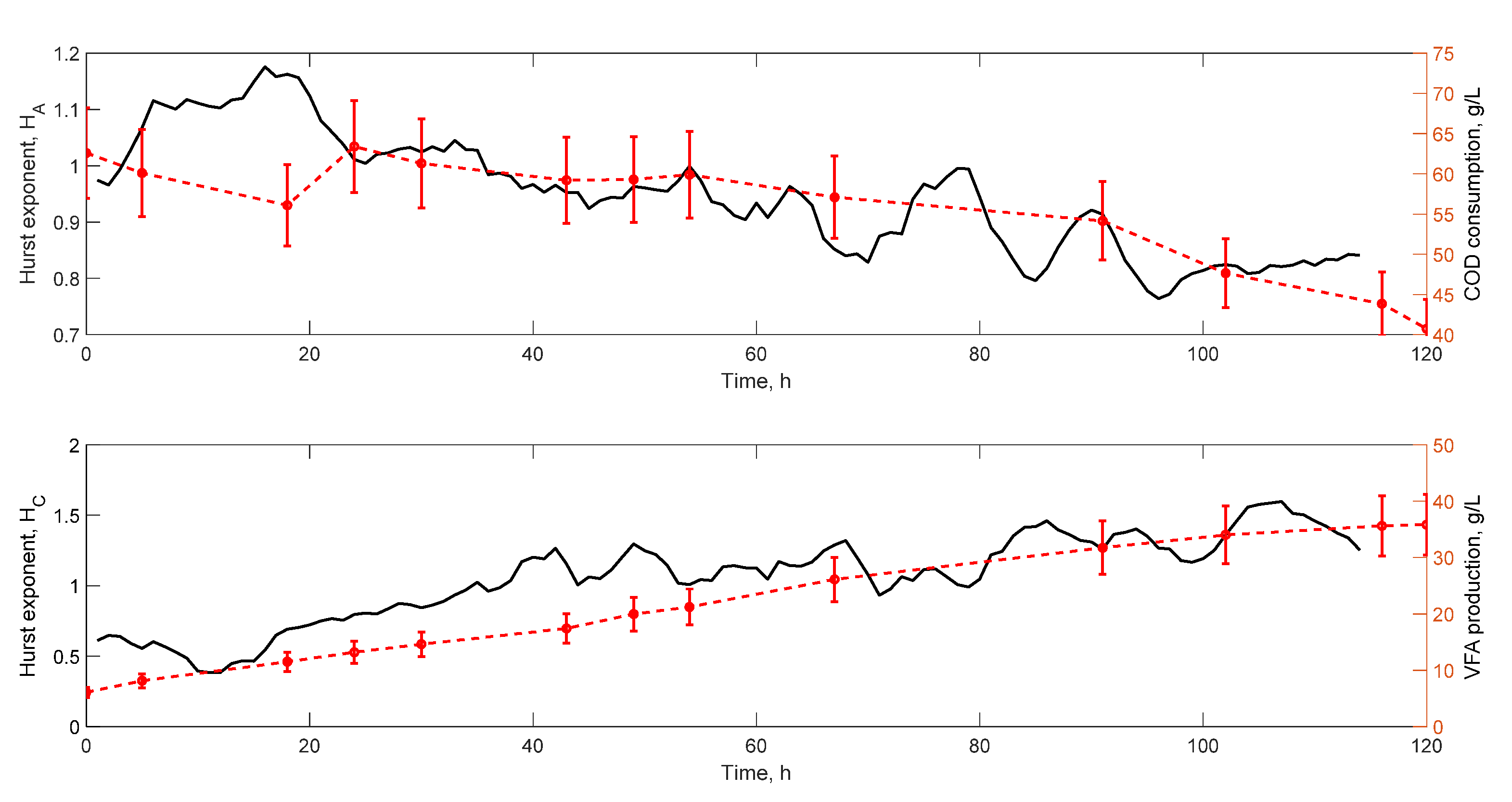
3.4. Fractal Analysis
4. Conclusions
Author Contributions
Funding
Acknowledgments
Conflicts of Interest
References
- Weiland, P.; Rozzi, A. The start-up, operation and monitoring of high rate anaerobic treatment systems: Discussers report. Water Sci. Technol. 1991, 24, 257–277. [Google Scholar] [CrossRef]
- Larroche, C.; Sanroman, M.A.; Du, G.; Pandey, A. Current Developments in Biotechnology and Bioengineering: Bioprocesses, Bioreactors and Controls; Elsevier: Amsterdam, The Netherlands, 2016. [Google Scholar]
- McCarty, P. Anaerobic waste treatment fundamentals. Part one: Chemistry and microbiology. Public Works 1964, 95, 107–112. [Google Scholar]
- Olsson, G.; Newell, B. Wastewater Treatment Systems: Modelling, Diagnosis and Control; IWA Publishing: London, UK, 2001. [Google Scholar]
- Jimenez, J.; Latrille, E.; Harmand, J.; Robles, A.; Ferrer, J.; Gaida, D.; Wolf, C.; Mairet, F.; Bernard, O.; Alcaraz-Gonzalez, V.; et al. Instrumentation and control of anaerobic digestion processes: A review and some research challenges. Rev. Environ. Sci. Bio/Technol. 2015, 14, 615–648. [Google Scholar] [CrossRef]
- Schügerl, K. Progress in monitoring, modeling and control of bioprocesses during the last 20 years. J. Biotechnol. 2001, 85, 149–173. [Google Scholar] [CrossRef]
- American Public Health Association; American Water Works Association; Water Pollution Control Federation; Water Environment Federation. Standard Methods for the Examination of Water and Wastewater; American Public Health Association: Washington, DC, USA, 1915. [Google Scholar]
- Hu, Z.; Grasso, D. Water analysis: Chemical oxygen demand. In Encyclopedia of Analytical Science, 2nd ed.; Elsevier Academic Press: Amsterdam, The Netherlands, 2005; pp. 325–330. [Google Scholar]
- Zhao, L.; Fu, H.Y.; Zhou, W.; Hu, W.S. Advances in process monitoring tools for cell culture bioprocesses. Eng. Life Sci. 2015, 15, 459–468. [Google Scholar] [CrossRef]
- Feitkenhauer, H.; von Sachs, J.; Meyer, U. On-line titration of volatile fatty acids for the process control of anaerobic digestion plants. Water Res. 2002, 36, 212–218. [Google Scholar] [CrossRef]
- Palacio-Barco, E.; Robert-Peillard, F.; Boudenne, J.L.; Coulomb, B. On-line analysis of volatile fatty acids in anaerobic treatment processes. Anal. Chim. Acta 2010, 668, 74–79. [Google Scholar] [CrossRef]
- Lamb, J.J.; Bernard, O.; Sarker, S.; Lien, K.M.; Hjelme, D.R. Perspectives of optical colourimetric sensors for anaerobic digestion. Renew. Sustain. Energy Rev. 2019, 111, 87–96. [Google Scholar] [CrossRef]
- Walker, M.; Zhang, Y.; Heaven, S.; Banks, C. Potential errors in the quantitative evaluation of biogas production in anaerobic digestion processes. Biores. Technol. 2009, 100, 6339–6346. [Google Scholar] [CrossRef] [Green Version]
- Biechele, P.; Busse, C.; Solle, D.; Scheper, T.; Reardon, K. Sensor systems for bioprocess monitoring. Eng. Life Sci. 2015, 15, 469–488. [Google Scholar] [CrossRef]
- Dochain, D. State and parameter estimation in chemical and biochemical processes: A tutorial. J. Process Cont. 2003, 13, 801–818. [Google Scholar] [CrossRef]
- Komives, C.; Parker, R.S. Bioreactor state estimation and control. Curr. Opin. Biotechnol. 2003, 14, 468–474. [Google Scholar] [CrossRef]
- Kadlec, P.; Gabrys, B.; Strandt, S. Data-driven soft sensors in the process industry. Comp. Chem. Eng. 2009, 33, 795–814. [Google Scholar] [CrossRef] [Green Version]
- Luttmann, R.; Bracewell, D.G.; Cornelissen, G.; Gernaey, K.V.; Glassey, J.; Hass, V.C.; Kaiser, C.; Preusse, C.; Striedner, G.; Mandenius, C.F. Soft sensors in bioprocessing: A status report and recommendations. Biotechnol. J. 2012, 7, 1040–1048. [Google Scholar] [CrossRef]
- Ali, J.M.; Hoang, N.H.; Hussain, M.A.; Dochain, D. Review and classification of recent observers applied in chemical process systems. Comp. Chem. Eng. 2015, 76, 27–41. [Google Scholar]
- Alexander, R.; Campani, G.; Dinh, S.; Lima, F.V. Challenges and opportunities on nonlinear state estimation of chemical and biochemical processes. Processes 2020, 8, 1462. [Google Scholar] [CrossRef]
- Méndez-Acosta, H.O.; Hernandez-Martinez, E.; Jáuregui-Jáuregui, J.A.; Alvarez-Ramirez, J.; Puebla, H. Monitoring anaerobic sequential batch reactors via fractal analysis of pH time series. Biotechnol. Bioeng. 2013, 110, 2131–2139. [Google Scholar] [CrossRef] [PubMed]
- Hernandez-Martinez, E.; Puebla, H.; Mendez-Acosta, H.O.; Alvarez-Ramirez, J. Fractality in pH time series of continuous anaerobic bioreactors for tequila vinasses treatment. Chem. Eng. Sci. 2014, 109, 17–25. [Google Scholar] [CrossRef]
- Besançon, G. Nonlinear Observers and Applications; Springer: Berling/Heidelberg, Germany, 2013; pp. 1–33. [Google Scholar]
- Meurer, T.; Graichen, K.; Gilles, E.D. Control and Observer Design for Nonlinear Finite and Infinite Dimensional Systems; Springer Science & Business Media: Berlin/Heidelberg, Germany, 2005. [Google Scholar]
- Alcaraz-González, V.; Steyer, J.P.; Harmand, J.; Rapaport, A.; González-Alvarez, V.; Pelayo-Ortiz, C. Application of a robust interval observer to an anaerobic digestion process. Dev. Chem. Eng. Mineral Process. 2005, 13, 267–278. [Google Scholar] [CrossRef]
- Morel, E.; Tartakovsky, B.; Guiot, S.R.; Perrier, M. Design of a multi-model observer-based estimator for anaerobic reactor monitoring. Comp. Chem. Eng. 2006, 31, 78–85. [Google Scholar] [CrossRef]
- Sbarciog, M.; Moreno, J.A.; Vande Wouwer, A. Application of super-twisting observers to the estimation of state and unknown inputs in an anaerobic digestion system. Water Sci. Technol. 2014, 69, 414–421. [Google Scholar] [CrossRef]
- Didi, I.; Dib, H.; Cherki, B. A Luenberger-type observer for the AM2 model. J. Process Cont. 2015, 32, 117–126. [Google Scholar] [CrossRef]
- Rodríguez, A.; Quiroz, G.; Femat, R.; Méndez-Acosta, H.O.; de León, J. An adaptive observer for operation monitoring of anaerobic digestion wastewater treatment. Chem. Eng. J. 2015, 269, 186–193. [Google Scholar] [CrossRef]
- Lara-Cisneros, G.; Aguilar-López, R.; Dochain, D.; Femat, R. On-line estimation of VFA concentration in anaerobic digestion via methane outflow rate measurements. Comp. Chem. Eng. 2016, 94, 250–256. [Google Scholar] [CrossRef]
- Chaib Draa, K.; Zemouche, A.; Alma, M.; Voos, H.; Darouach, M. A discrete-time nonlinear state observer for the anaerobic digestion process. Int. J. Robust Nonlin. Cont. 2019, 29, 1279–1301. [Google Scholar] [CrossRef]
- Lara-Cisneros, G.; Dochain, D. Software sensor for online estimation of the VFA’s concentration in anaerobic digestion processes via a high-order sliding mode observer. Ind. Eng. Chem. Res. 2018, 57, 14173–14181. [Google Scholar] [CrossRef]
- Dewasme, L.; Sbarciog, M.; Rocha-Cózatl, E.; Haugen, F.; Wouwer, A.V. State and unknown input estimation of an anaerobic digestion reactor with experimental validation. Cont. Eng. Pract. 2019, 85, 280–289. [Google Scholar] [CrossRef]
- Duan, Z.; Kravaris, C. Nonlinear observer design for two-time-scale systems. AIChE J. 2020, 66, e16956. [Google Scholar] [CrossRef]
- Liu, Y.Y.; Slotine, J.J.; Barabási, A.L. Observability of complex systems. Proc. Natl. Acad. Sci. USA 2013, 110, 2460–2465. [Google Scholar] [CrossRef] [Green Version]
- Chen, C.T.; Chen, C.T. Linear System Theory and Design; Holt, Rinehart and Winston: New York, NY, USA, 1984. [Google Scholar]
- Montanari, A.N.; Aguirre, L.A. Observability of network systems: A critical review of recent results. J. Control Automat. Elect. Sys. 2020, 31, 1348–1374. [Google Scholar] [CrossRef]
- Golabgir, A.; Hoch, T.; Zhariy, M.; Herwig, C. Observability analysis of biochemical process models as a valuable tool for the development of mechanistic soft sensors. Biotechnol. Progress 2015, 31, 1703–1715. [Google Scholar] [CrossRef] [PubMed]
- López, E.; Gómez, L.M.; Alvarez, H. A set-theoretic approach to observability and its application to process control. J. Process Cont. 2019, 80, 15–25. [Google Scholar] [CrossRef]
- Nahar, J.; Liu, J.; Shah, S.L. Parameter and state estimation of an agro-hydrological system based on system observability analysis. Comp. Chem. Eng. 2019, 121, 450–464. [Google Scholar] [CrossRef]
- Holubar, P.; Zani, L.; Hager, M.; Fröschl, W.; Radak, Z.; Braun, R. Start-up and recovery of a biogas-reactor using a hierarchical neural network-based control tool. J. Chem. Technol. Biotechnol. 2003, 78, 847–854. [Google Scholar] [CrossRef]
- Ozkaya, B.; Demir, A.; Bilgili, M.S. Neural network prediction model for the methane fraction in biogas from field-scale landfill bioreactors. Environ. Model. Soft. 2007, 22, 815–822. [Google Scholar] [CrossRef]
- Strik, D.P.; Domnanovich, A.M.; Zani, L.; Braun, R.; Holubar, P. Prediction of trace compounds in biogas from anaerobic digestion using the MATLAB Neural Network Toolbox. Environ. Model. Soft. 2005, 20, 803–810. [Google Scholar] [CrossRef]
- Kazemi, P.; Steyer, J.P.; Bengoa, C.; Font, J.; Giralt, J. Robust data-driven soft sensors for online monitoring of volatile fatty acids in anaerobic digestion processes. Processes 2020, 8, 67. [Google Scholar] [CrossRef] [Green Version]
- Gosak, M.; Markovič, R.; Dolenšek, J.; Rupnik, M.S.; Marhl, M.; Stožer, A.; Perc, M. Network science of biological systems at different scales: A review. Phys. Life Rev. 2018, 24, 118–135. [Google Scholar] [CrossRef]
- Jalan, S.; Yadav, A.; Sarkar, C.; Boccaletti, S. Unveiling the multi-fractal structure of complex networks. Chaos Solitons Fractals 2017, 97, 11–14. [Google Scholar] [CrossRef] [Green Version]
- Sánchez-García, D.; Hernández-García, H.; Mendez-Acosta, H.O.; Hernández-Aguirre, A.; Puebla, H.; Hernández-Martínez, E. Fractal analysis of pH time-series of an anaerobic digester for cheese whey treatment. Int. J. Chem. Reactor Eng. 2018, 16. [Google Scholar] [CrossRef]
- Carvalho, F.; Prazeres, A.R.; Rivas, J. Cheese whey wastewater: Characterization and treatment. Sci. Total Environ. 2013, 445, 385–396. [Google Scholar] [CrossRef]
- Escalante, H.; Castro, L.; Amaya, M.P.; Jaimes, L.; Jaimes-Estévez, J. Anaerobic digestion of cheese whey: Energetic and nutritional potential for the dairy sector in developing countries. Waste Manag. 2018, 71, 711–718. [Google Scholar] [CrossRef]
- B-Arrollo, C.; Lara-Musule, A.; Alvarez-Sanchez, E.; Trejo-Aguilar, G.; Bastidas-Oyanedel, J.R.; Hernandez-Martinez, E. An unstructured model for anaerobic treatment of raw cheese whey for volatile fatty acids production. Energies 2020, 13, 1850. [Google Scholar] [CrossRef]
- Fridman, L.; Shtessel, Y.; Edwards, C.; Yan, X.G. Higher-order sliding-mode observer for state estimation and input reconstruction in nonlinear systems. Int. J. Robust Nonlin. Contr. 2008, 18, 399–412. [Google Scholar] [CrossRef]
- Chawengkrittayanont, P.; Pukdeboon, C. Continuous higher order sliding mode observers for a class of uncertain nonlinear systems. Trans. Instit. Meas. Cont. 2019, 41, 717–728. [Google Scholar] [CrossRef]
- Campos-Dominguez, A.; Ceballos-Ceballos, Y.; Velazquez-Camilo, O.; Puebla, H.; Hernandez-Martinez, E. Fractal analysis of temperature time series from batch sugarcane crystallization. Fractals 2019, 27, 1950004. [Google Scholar] [CrossRef]
- Hernandez-Martinez, E.; Perez-Muñoz, T.; Velasco-Hernandez, J.X.; Altamira-Areyan, A.; Velasquillo-Martinez, L. Facies recognition using multifractal Hurst analysis: Applications to well-log data. Math. Geosci. 2013, 45, 471–486. [Google Scholar] [CrossRef]
- Mandelbrot, B.B. The Fractal Geometry of Nature; WH freeman: New York, NY, USA, 1982. [Google Scholar]
- Korbicz, J.; Witczak, M.; Puig, V. LMI-based strategies for designing observers and unknown input observers for non-linear discrete-time systems. Bull. Polish Acad. Sci. Tech. Sci. 2007, 55, 31–42. [Google Scholar]


| NMSE | ELO | High-Order SMO |
|---|---|---|
| CH4 | 0.01006 | 0.0079 |
| VFA (A) | 0.0269 | 0.0304 |
| S1 | 0.0601 | 0.0601 |
| S2 | 0.01502 | 0.0153 |
Publisher’s Note: MDPI stays neutral with regard to jurisdictional claims in published maps and institutional affiliations. |
© 2021 by the authors. Licensee MDPI, Basel, Switzerland. This article is an open access article distributed under the terms and conditions of the Creative Commons Attribution (CC BY) license (http://creativecommons.org/licenses/by/4.0/).
Share and Cite
Flores-Mejia, H.; Lara-Musule, A.; Hernández-Martínez, E.; Aguilar-López, R.; Puebla, H. Indirect Monitoring of Anaerobic Digestion for Cheese Whey Treatment. Processes 2021, 9, 539. https://doi.org/10.3390/pr9030539
Flores-Mejia H, Lara-Musule A, Hernández-Martínez E, Aguilar-López R, Puebla H. Indirect Monitoring of Anaerobic Digestion for Cheese Whey Treatment. Processes. 2021; 9(3):539. https://doi.org/10.3390/pr9030539
Chicago/Turabian StyleFlores-Mejia, Hilario, Antonio Lara-Musule, Eliseo Hernández-Martínez, Ricardo Aguilar-López, and Hector Puebla. 2021. "Indirect Monitoring of Anaerobic Digestion for Cheese Whey Treatment" Processes 9, no. 3: 539. https://doi.org/10.3390/pr9030539