Testing the Accuracy of the Cell-Set Model Applied on Vane-Type Sub-Boundary Layer Vortex Generators

Abstract

Vortex Generators (VGs) are applied before the expected region of separation of the boundary layer in order to delay or remove the flow separation. Although their height is usually similar to that of the boundary layer, in some applications, lower VGs are used, Sub-Boundary Layer Vortex Generators (SBVGs), since this reduces the drag coefficient. Numerical simulations of sub-boundary layer vane-type vortex generators on a flat plate in a negligible pressure gradient flow were conducted using the fully resolved mesh model and the cell-set model, with the aim on assessing the accuracy of the cell-set model with Reynolds-Averaged Navier-Stokes (RANS) and Large Eddy Simulation (LES) turbulence modelling techniques. The implementation of the cell-set model has supposed savings of the 40% in terms of computational time. The vortexes generated on the wake behind the VG; vortical structure of the primary vortex; and its path, size, strength, and produced wall shear stress have been studied. The results show good agreements between meshing models in the higher VGs, but slight discrepancies on the lower ones. These disparities are more pronounced with LES. Further study of the cell-set model is proposed, since its implementation entails great computational time and resources savings.

1. Introduction

Vortex Generators (VGs) are passive flow control devices, whose objective is to delay or remove the flow separation, transferring the energy generated from the outer region to the boundary layer region. They are small vanes placed before the expected region of separation of the boundary layer. They are usually mounted in pairs, with an incident angle with the oncoming flow. Regarding their shape, VGs can be of various geometries, but they are mainly triangular or rectangular. Their height is typically similar to the boundary layer thickness where the VG is applied, in order to ensure a good interaction between the boundary layer and the vortex generated in the VG. However, since tall VGs lead to high drag forces, VGs with smaller heights than the local boundary thickness, i.e., Sub-Boundary-Layer Vortex Generators (SBVGs), are used in many applications, see Ashill et al. [1,2]. Aramendia et al. [3,4] comprehensively reviewed the available flow control devices, including VGs, and Lin [5] conducted an in-depth review of the control of flow separation in the boundary layer using SBVGs.

Since their introduction by Taylor [6] in the late 1940s, VGs have been used in a wide range of industries for numerous applications. Among these industries, aerodynamics and thermodynamics are the most remarkable. Øye [7] and Miller [8] implemented VGs on 1 MW and 2.5 MW wind turbines, respectively. Heyes and Smith [9] added VGs of numerous shapes on the wing tip of an aircraft, and Tai [10] studied the effect of Micro-Vortex Generators (MVGs) on V-22 aircraft. All of them showed a significant aerodynamic performance improvement when implementing VGs.

Another sector in which VGs are widely used is thermodynamics. Currently, major efforts are being made in the thermodynamics field to increase heat and mass transfer, see Agnew et al. [11]. For this reason, numerous authors have implemented in different thermodynamic systems. For example, Joardar and Jacobi [12] studied the heat transfer and pressure drop of a heat exchanger before and after the addition of VGs, showing an increase of the heat transfer coefficient between 16.5% and 44% with a single VG pair and between 30% and 68.8% with 3 VG pairs.

Although many studies use experimental techniques, the use of Computational Fluid Dynamics (CFD) tools for performing numerical studies is becoming a very popular choice for studying VGs. CFD studies of VGs are currently focused on two main goals. The first goal is to optimize the position and distribution of VGs, see the studies of Subbiah et al. [13] and Yu et al. [14]. The second goal is to analyze the swirling vortexes generated on the wake behind the VG, see the studies of Carapau and Janela [15] and Sheng et al. [16] about this phenomenon.

Many authors have studied SBVGs using CFD. Ibarra-Udaeta et al. [17] and Martinez-Filgueira et al. [18] analyzed the vortices generated by rectangular vane-type SBVGs on a flat plate under negligible pressure gradient flow conditions. They analyzed VGs with heights equal to 0.2, 0.4, 0.6, 0.8, 1, and 1.2 δ and incident angles equal to 10°, 15°, 18°, and 20°. Fernandez-Gamiz et al. [19] studied three different SBVGs with heights of 0.21, 0.25, and 0.31 δ and an incident angle equal to 18°. Gutierrez-Amo et al. [20] analyzed a rectangular, a triangular, and a symmetrical NACA0012 SBVG. Fully resolved mesh modelling technique was used in all the mentioned studies, and all of them showed good agreements with experimental data.

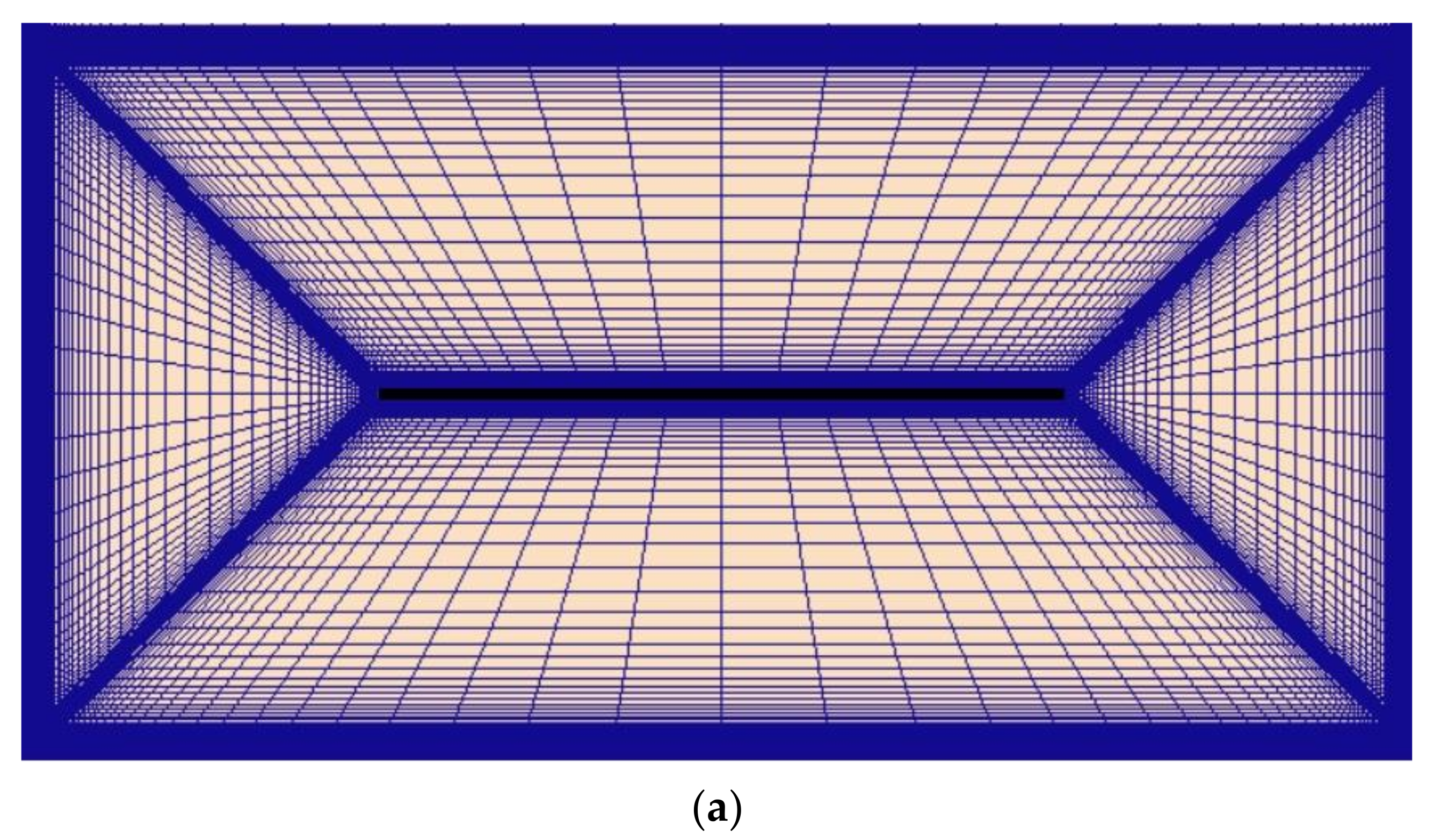
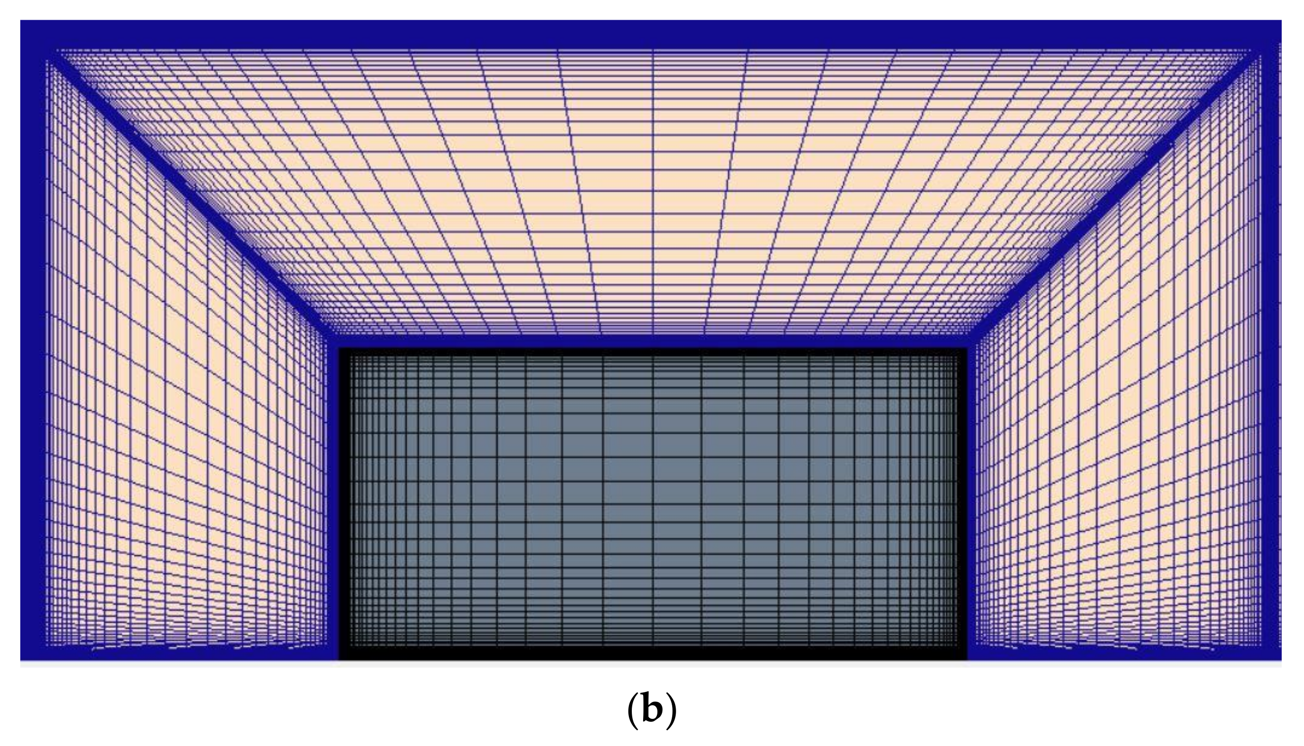
The main disadvantage of the fully resolved mesh model is the fine mesh that requires to accurately capture the physical phenomena, especially in the near-VG region and in the wake behind the VG. For that reason, numerous authors [21,22,23] have implemented alternative models. The majority of these models are based on the BAY model developed by Bender et al. [24], which models the force produced by a VG. Errasti et al. [25] implemented the jBAY source-term model developed by Jirasek [26] in vane-type SBVGs under adverse pressure flow conditions and showed accurate results in terms of vortex path, vortex decay, and vortex size.

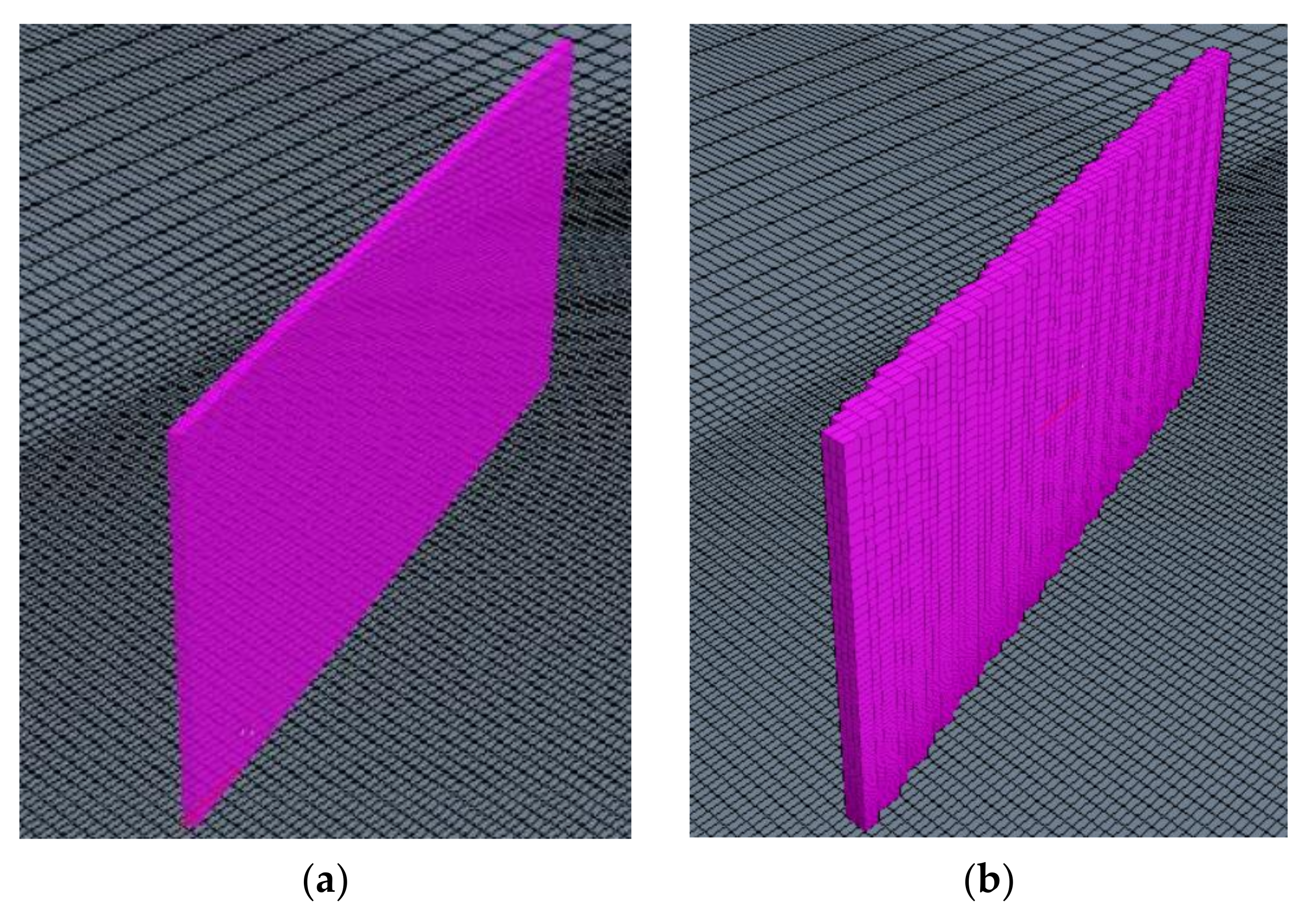
The cell-set model is another alternative model, which consists of leveraging the previously generated mesh to build the desired geometry. Besides the advantages that the cell-set model provides over the fully resolved mesh model, there are not many studies in which this model has been applied. Ballesteros-Coll et al. [21,27] used the cell-set model to generate Gurney flaps and microtabs on DU91W250 airfoils, and Ibarra-Udaeta et al. [28] modelled conventional vane-type VGs with this model.

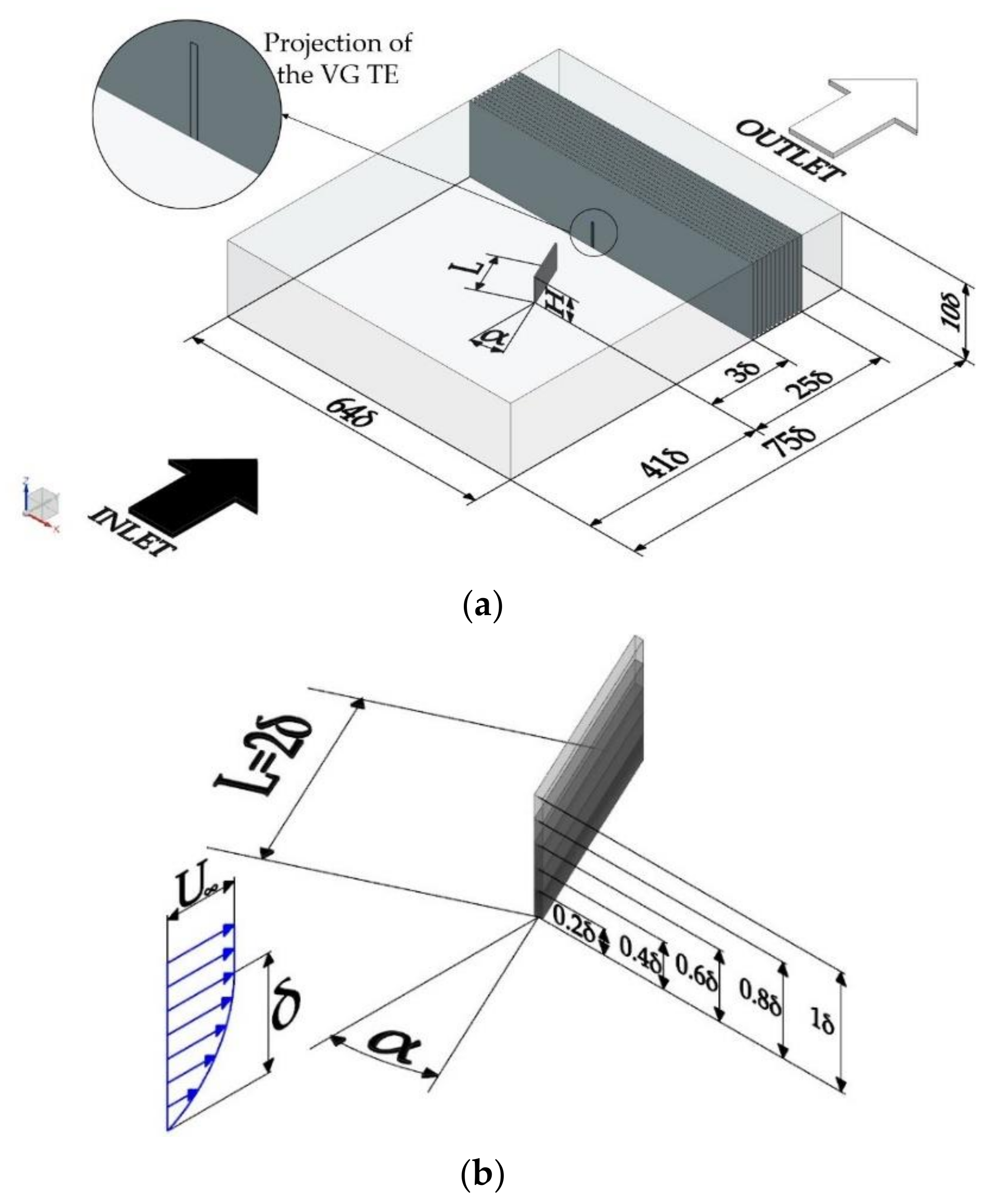
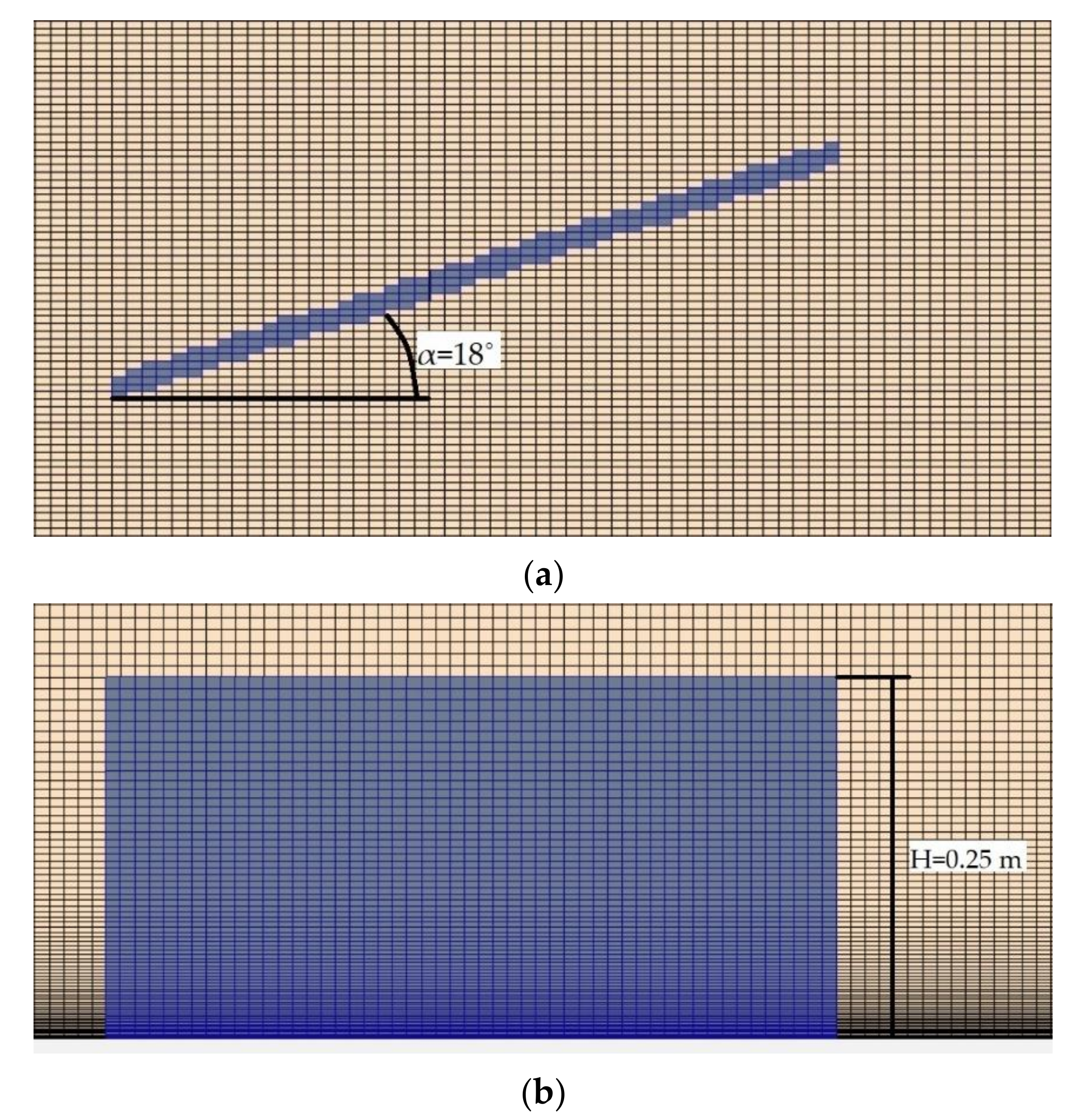
The goal of the present paper is to evaluate the accuracy of the cell-set model applied on SBVGs with heights of 0.2, 0.4, 0.6, 0.8, and 1 δ. For that purpose, CFD simulations of SBVGs on a flat plate in a negligible streamwise pressure gradient flow conditions are conducted using the fully resolved mesh model and the cell-set model, and the results obtained with the fully resolved mesh model are taken as benchmark. With the purpose of testing the cell-set model with RANS and LES, both models are used to conduct the simulations.

The remainder of the manuscript is structured as follows: Section 2 provides a general description of the used numerical domain and meshing models. Section 3 explains the results obtained in the present work. Finally, Section 4 summarizes the main conclusions reached from the results and future directions.

2. Numerical Setup

CFD simulations of sub-boundary layer vane-type VGs on a flat plate in a negligible streamwise pressure gradient flow were conducted with the intention of investigating the accuracy cell-set model. Star CCM+v14.02.012 [29] CFD commercial code was used to conduct all the simulations.

2.1. Computational Domain and Physic Models

The computational domain consists of a block with a rectangular VG situated on its lower surface. The flow goes from the upstream part of the block to its downstream part; hence, they are set as inlet and outlet, respectively. The bottom surface of the block and the faces of the VG are set as no-slip walls, and symmetry plane conditions are assigned to the rest of the surfaces, ensuring that the flow is not affected by their presence. The computational domain has been designed to ensure that the boundary layer thickness (δ) at the location of the VG is equal to 0.25 m.

Regarding the fluid, an incompressible turbulent flow is considered, in a steady-state with RANS and in an unsteady-state with LES. According to expression (1), the Reynolds number (Re) of this flow is around 27,000.

$$Re=\frac{U_{\infty }·\delta }{v},$$

(1)

where $v$ refers to the kinematic viscosity and $U_{\infty }$ to the free stream velocity of the flow, which is set at 20 m/s for this study.

As the objective of this paper is to analyze the cell-set model on SBVGs, 10 different SBVGs are considered. Five different VG heights (H), 0.2, 0.4, 0.6, 0.8, and 1 δ, and two different incident (α) angles, 18° and 25°, are considered. The length (L) of the VG is equal to 2 δ for every case. More information about the VGs and the computational domain is shown in

Table 1. Vortex Generator (VG) dimensions.

VG Height (H)	Vane Height to Boundary Layer Thickness (H/δ)	VG Length (L)	Aspect Ratio
0.05 m	0.2	0.50 m	10
0.10 m	0.4	0.50 m	5
0.15 m	0.6	0.50 m	3.33
0.20 m	0.8	0.50 m	2.5
0.25 m	1	0.50 m	2

and Figure 1.

For the simulations in which α is equal to 18°, Menter’s k-ω SST (Shear Stress Transport) [30]. RANS-based turbulence model is selected. This model has been selected since, as demonstrated by Allan et al. [31], SST models provide more accurate vortex trajectory and streamwise peak vorticity predictions than other RANS models. In contrast, Urkiola et al. [32] showed that when working with high incident angles, RANS-based models are not able to capture flow characteristics as accurately as when working with low incident angles. Hence, for the simulations in which the incident angle is equal to 25°, LES Smagorinsky SGS (sub-grid-scale) [33] model is selected. Furthermore, this selection of turbulence models allows the cell-set model to be analyzed using both RANS and LES.

For data extraction, 12 spanwise planes normal to the streamwise direction located on the wake behind the VG are considered. These planes are located from 3 to 25 δ from the LE (Leading Edge), separated 2 δ between each other.

2.2. Fully Resolved Mesh Model

Five different structured meshes of around 11.5 million hexahedral cells were generated, one for each VG height. In all the cases, the normalized height of the closest cell to the wall (Δz/δ) was set at $1.5{\times 10}^{-6}$. For the generation of these meshes, the procedure described by Urkiola et al. [32] was followed. In order to obtain more accurate results in the near-VG region, these meshes are refined in this zone. The meshes were rotated to obtain the desired incident angles (α = 18° and α = 25°). Figure 2 shows the mesh refinement around the VG for the case H = 1 δ.

The skewness angle, volume change, and face validity cell quality parameters have been selected to assess the quality of the tested meshes. The skewness angle is the angle between a face normal vector of a cell and the vector connecting the centroids of this cell and the neighbor cells. The volume change is the ratio of the volume of a cell to that of its largest neighbor. The face validity is a measure of the correctness of the face normal relative to its attached cell centroid.

According to [29], the skewness angle should be as low as possible, and cells with a skewness angle greater that 85° could result in solver convergence issues, so they are considered low-quality cells. These problems appear since the diffusion term for transported scalar variables contains in its denominator the dot product between the face normal vector and the vector connecting the centroids, and therefore, skewness angles close to 90° imply very high values of this term. The volume change ratio should be close to 1, since large jump in volume from one cell to its neighbor can cause inaccuracies and instability in the solvers. Therefore, cells with volume changes below 0.01 are considered inadequate. The face validity must be equal to 1, since different values mean that the face normals do not point away from the cell centroid correctly, and values below 0.5 signify a negative volume cell. As

Table 2. Cell quality parameters of the used meshes with the fully resolved mesh model.

VG Height	Maximum Skewness Angle	Minimum Volume Change	Minimum Face Validity
0.2 δ	81.1°	0.029	1
0.4 δ	75.1°	0.029	1
0.6 δ	66.7°	0.029	1
0.8 δ	64.8°	0.03	1
1 δ	65.3°	0.03	1

shows, all the meshes fulfill these criteria.

To verify sufficient mesh resolution, two different procedures were followed, one for each turbulence model. Both mesh resolution studies were applied for the case H = 1 δ. For RANS, the General Richardson Extrapolation method [34] was performed, applied to lift and drag forces of the VG. This method consists of estimating the value of the analyzed parameter when the cell quantity tends to infinite from a minimum of three meshes. For this study, a coarse mesh (0.2 million cells), a medium mesh (1.4 million cells), and a fine mesh (the previously explained mesh, 11.5 million cells) were considered. As summarized in

Table 3. Mesh verification for Reynolds-Averaged Navier-Stokes (RANS).

Variable	Mesh Resolution			Richardson Extrapolation
	Coarse (N)	Medium (N)	Fine (N)	RE (N)	P	R
Drag force	98.0699	89.8929	87.199	85.875	1.6018	0.329
Lift force	261.605	247.715	241.39	236.1	1.135	0.455

, the convergence condition, which should be between 0 and 1 to ensure a monotonic convergence, is fulfilled, and the estimated values (RE) of the evaluated parameters are close to the ones obtained with the fine mesh. Therefore, the mesh is suitable for RANS simulations.

In LES, Taylor length-scale (λ) was examined to verify sufficient mesh resolution. According to Kuczaj et al. [35], the mesh resolution ($\Delta =\sqrt[3]{V_{cell}}$) should at least be in order of λ to completely solve the Taylor length-scale. As explained in [35], Taylor length-scale calculation procedure consists of obtaining the autocorrelation function from the Taylor expansion coefficient, then, calculating the Taylor time-scale, and finally, estimating λ from the Taylor hypothesis [36]. This method has been applied on the wake behind the VG, at y/δ = 1, since this area is expected to be the area where the effects of the turbulence are most noticeable, and therefore, the area where the best resolution is required. As Figure 3 shows that the criteria proposed by Kuczaj et al. [35] is fulfilled along the whole wake behind the VG, which means that the mesh is suitable for LES simulations.

2.3. Cell-Set Model

In the present work, the accuracy of the cell-set model applied on sub-boundary layer VGs is evaluated. This model consists of generating the desired geometry in a mesh that initially does not contain such geometry. To apply the cell-set model, the place where the geometry should be located in the mesh is indicated, as displayed in Figure 4a. Later, the cells that correspond to this geometry are selected by means of their cell ID. Finally, with the selected cells a new cell-set region is created, as shown in Figure 4b, and wall conditions are assigned to this new region.

With the cell-set model, meshes of around 7.2 million cells have been generated. Thus, the meshes are coarser with this model than with the fully resolved mesh model. In addition, the mesh design and generation processes are faster with the cell-set model. As in the fully resolved mesh, Δz/δ is equal to $1.5{\times 10}^{-6}$. Figure 5 shows the top and side views of the VG generated with the cell-set model for H = 1 δ and α = 18°.

As with the fully resolved mesh model, the quality of the meshes generated with the cell-set model has been evaluated with skewness angle, volume change and face validity parameters. As shown in

Table 4. Cell quality parameters of the used meshes with the cell-set model.

VG Height	Maximum Skewness Angle	Minimum Volume Change	Minimum Face Validity
0.2 δ	83.8°	0.365	1
0.4 δ	83.8°	0.365	1
0.6 δ	87.2°	0.359	1
0.8 δ	81.5°	0.355	1
1 δ	80.6°	0.352	1

, and according to the previously explained criteria, the cell quality of the meshes generated with the cell-set model is adequate.

To verify sufficient mesh resolution, as with the fully resolved mesh model, two different procedures have been followed, one for each turbulence model. In both cases, the mesh verification has been performed with the H = 1 δ case. For RANS, the General Richardson Extrapolation method has been applied. However, in this case, the three meshes are made of 7.2 million cells (fine mesh), 3.6 million cells (medium mesh), and 1.8 million cells (coarse mesh). As

Table 5. Mesh verification for RANS.

Variable	Mesh Resolution			Richardson Extrapolation
	Coarse (N)	Medium (N)	Fine (N)	RE (N)	P	R
Drag force	101.632	98.1029	96.3945	94.5856	1.0466	0.484
Lift force	259.1973	252.912	248.5026	237.7241	0.0495	0.7015

shows, the results fulfill the convergence condition. Thus, the mesh generated using the cell-set model is adequate for RANS simulations.

For LES simulations, Taylor length-scale (λ) is examined to verify sufficient mesh resolution. As shown in Figure 6, the mesh satisfies the criteria proposed by Kuczaj et al. [35] on the whole wake behind the VG, and therefore, it is suitable for LES simulations.

3. Results and Discussion

In this study, the vortices generated in the wake behind the VGs have been analyzed. Moreover, an exhaustive analysis of the primary vortex has been performed, studying its path, size, and strength and the wall shear stress behind it.

For the interpretation of RANS results, the last obtained values have been considered, whereas for the results of LES simulations, the average values of 2 s of simulation have been considered, after the flow is completely developed.

Parallel computing with 56 Intel Xeon 5420 cores and 45 GB of RAM were used to carry out all the simulations. Simulations performed with fully resolved mesh modelling were run for about 47 h using the RANS turbulence model and for around 184 h using the LES model. In contrast, simulations in which cell-set modelling was applied were run for approximately 28 h for RANS and 111 h for LES.

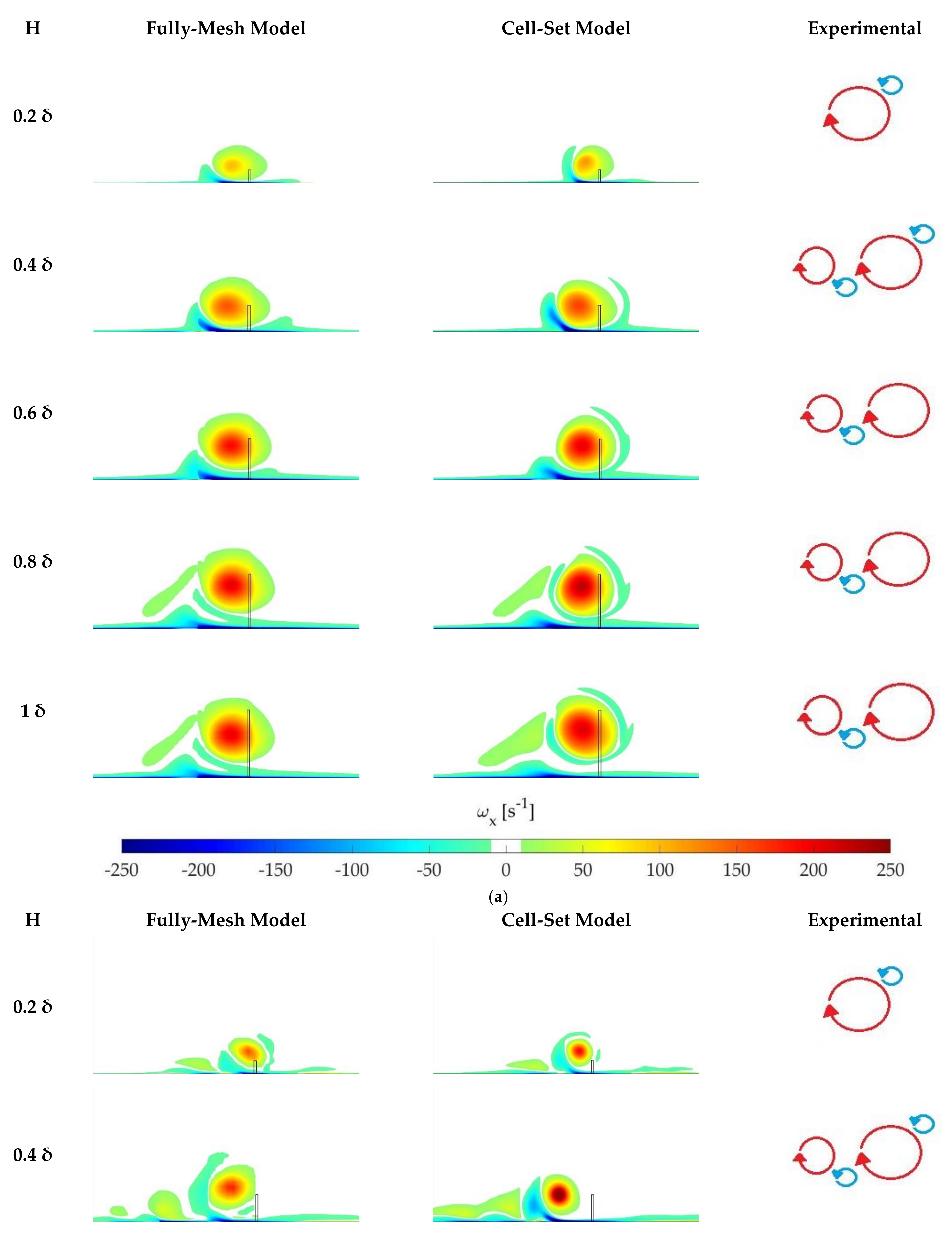
3.1. Vortex Structure Regimes in the Wake

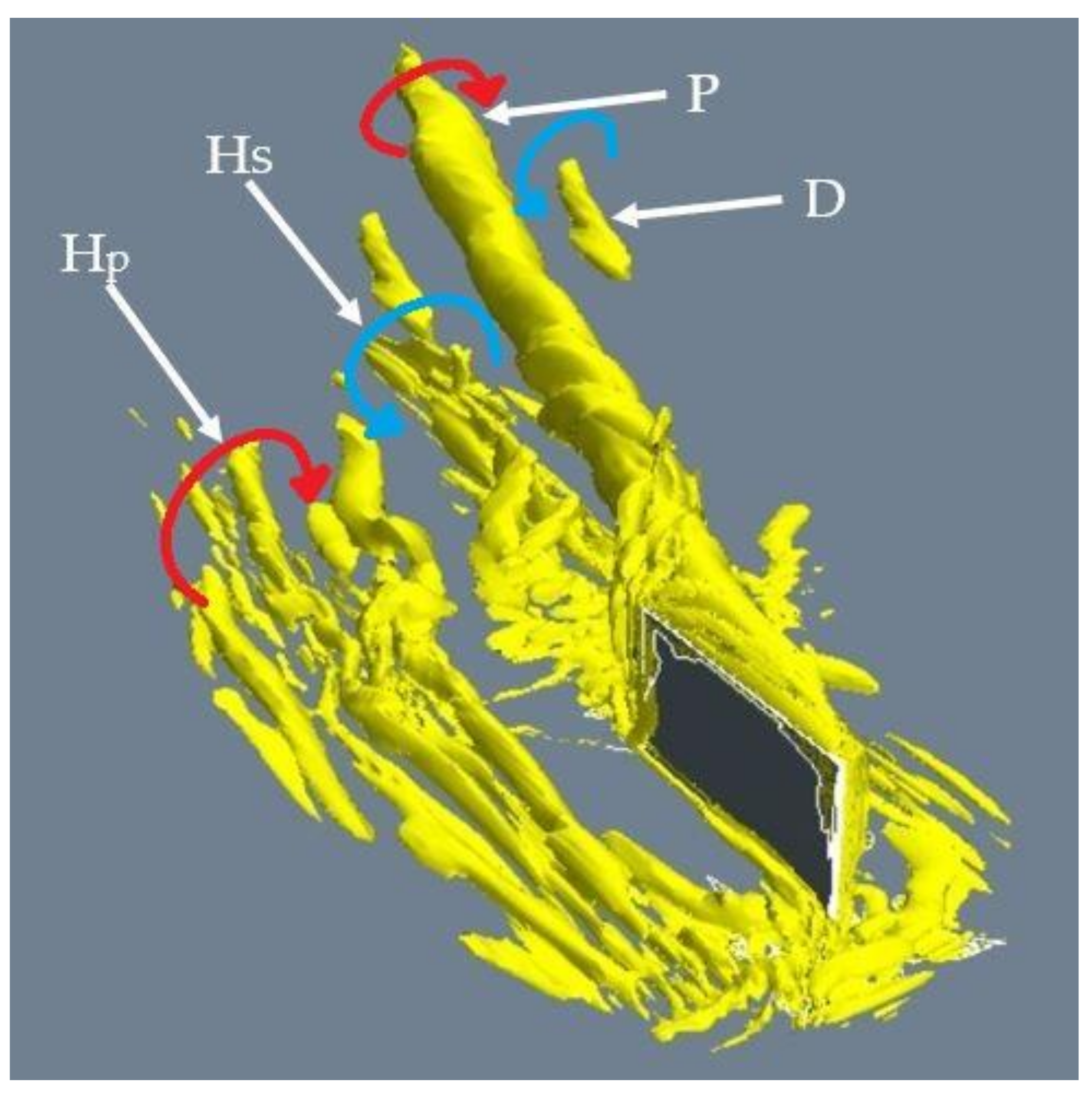
As measured by Velte [37], two basic vortex mechanism appear in the wake behind the VG. The main vortex system is composed of a primary vortex (P), which is formed on the wing tip, and a horseshoe vortex, which is generated from the rollup vortex around the LE of the VG. This horseshoe vortex is divided in two sides, the pressure side (Hp) and the suction side (Hs). As the primary vortex is stronger than these sides, the primary vortex pulls the suction side. As the primary vortex and the pressure side have the same sign, the pressure side remains undisturbed.

The secondary vortex structure is created by the local separation of the boundary layer in the lateral direction between the primary vortex and the wall. Due to the dragging of the suction side by the primary vortex, the primary vortex becomes stronger, the boundary layer region grows, and finally detaches, forming a discrete vortex (D). Figure 7 shows a representation of the primary and secondary vortexes.

Nevertheless, Velte [37] showed that these structures can vary, depending on the incident angle and the height of the VG. Figure 8 displays a comparison of the vortical structures predicted by the numerical simulations with both studied models at a distance of 5 δ from the VG Trailing Edge (TE), and the vortical structures measured by Velte [37].

Regarding the main vortex structure, the results show that both RANS and LES are able to accurately predict the primary vortex with the fully resolved mesh model and the cell-set model. In LES simulations, the horseshoe vortex, which is expected to appear in VGs with heights above 0.4 δ, is predicted for all the heights, including 0.2 δ. In contrast, RANS is not able to capture the pressure side of this horseshoe vortex for heights below 0.8 δ.

The largest discrepancies between the simulations and the experimental results appear in the secondary vortex structure. This vortex structure is expected to appear in VGs whose heights are below 0.4 δ. In LES, this vortex is only visible for H = 0.2 δ with the fully resolved mesh model. This vortex is not predicted in RANS for neither height.

Despite showing different values, the fully resolved mesh model and the cell-set model predict very similar vortexes in terms of vortex shape and direction.

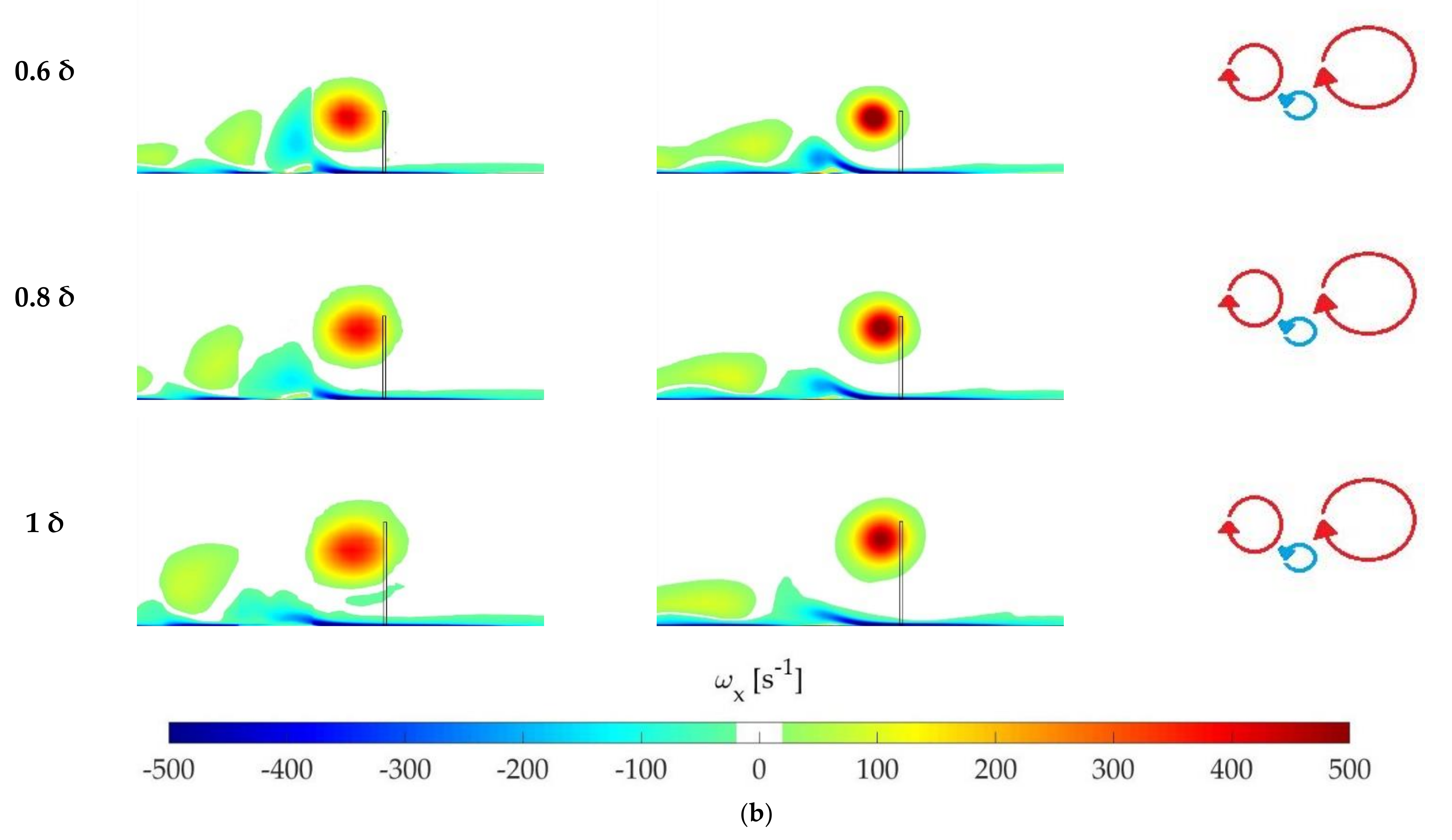
3.2. Vortical Structure of the Primary Vortex

The Q-criterion [38] method has been used to compare qualitatively the primary vortex generated by each VG in terms of shape and size. This method visualizes structures of the flow, and its value is defined by $Q=\frac{1}{2}\left({\Vert \Omega \Vert }^2-{\Vert S\Vert }^2\right)$, where Ω is the spin tensor and S the strain-rate tensor. As the value of Q is set at Q = 2500 s⁻², the vortical structures are displayed. Figure 9 shows the representation of the primary vortex at 5 δ from the VG TE by means of the Q-criterion.

The results show that for α = 18°, the taller the VG, the larger the vortex. However, for α = 25°, although this also occurs, the differences between heights are smaller, with the size of the vortices being more similar than when α = 18°.

With RANS, even if they have the same circular shape, the vortexes predicted by the cell-set model are larger than the ones predicted by the fully resolved mesh model. With LES, generally, the vortexes predicted by the cell-set model are smaller than those predicted by the fully resolved mesh model. In this case, slight disparities between models are visible in terms of vortex shape, which are attributed to the unsteadiness of the flow.

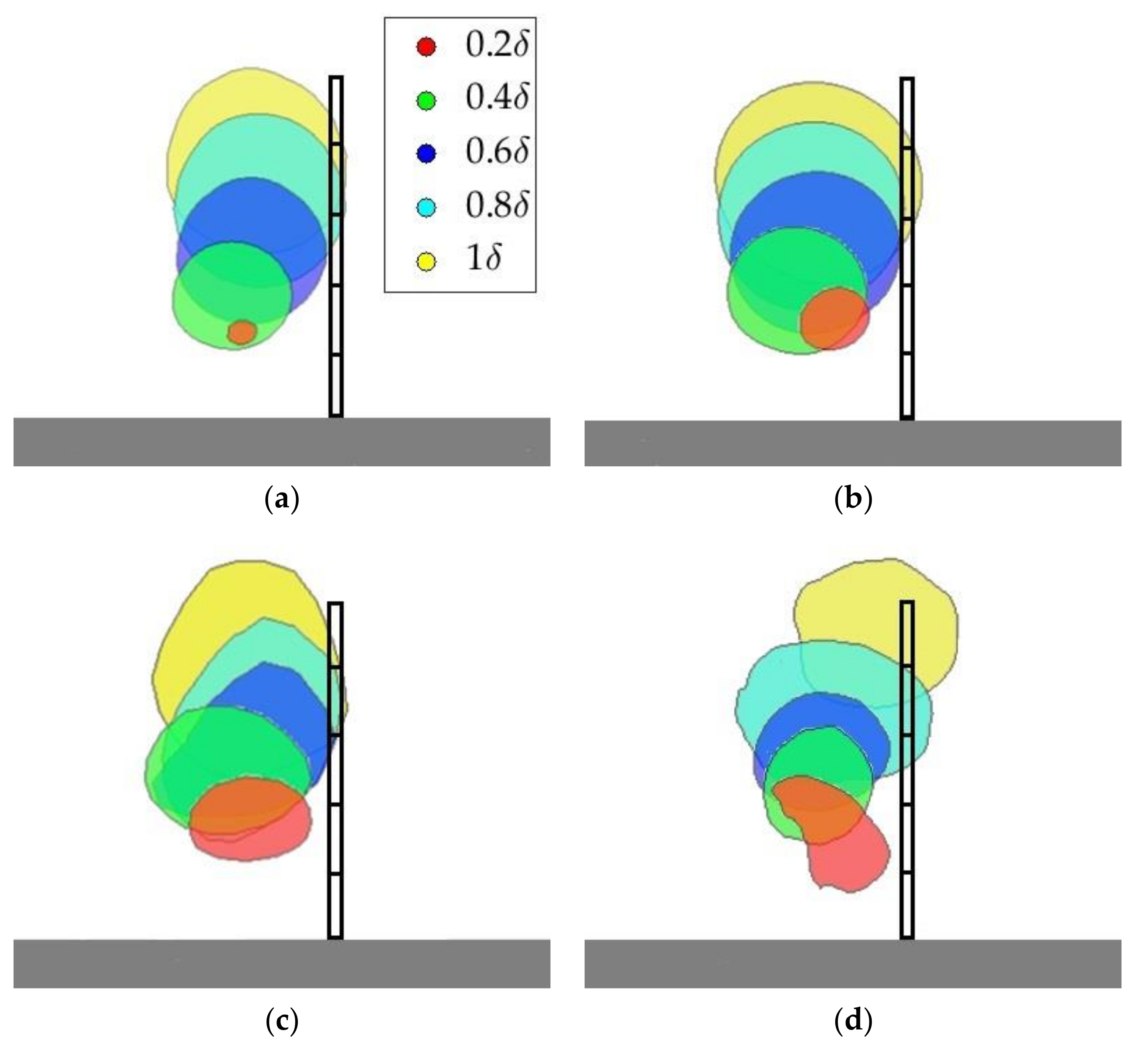
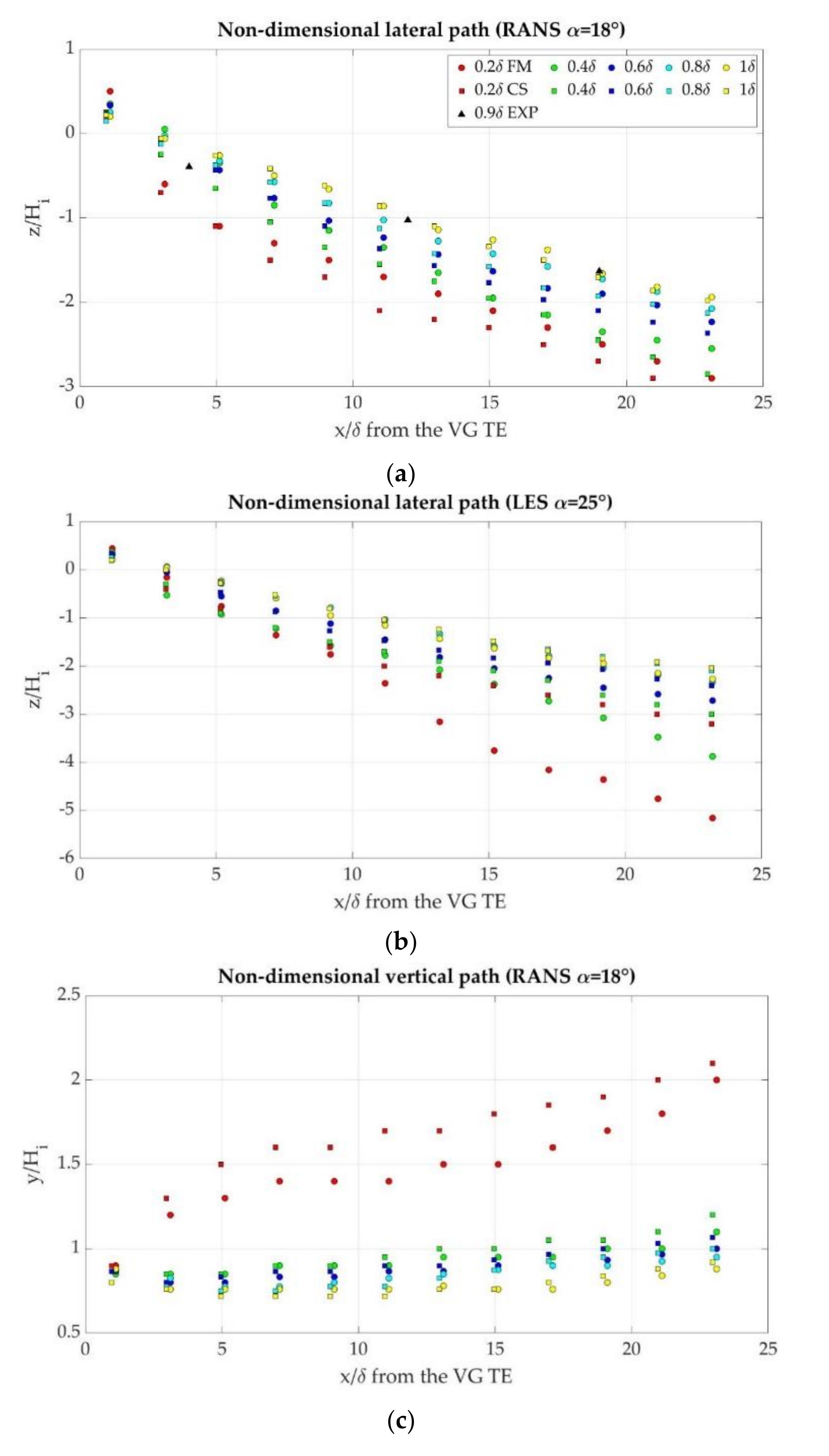
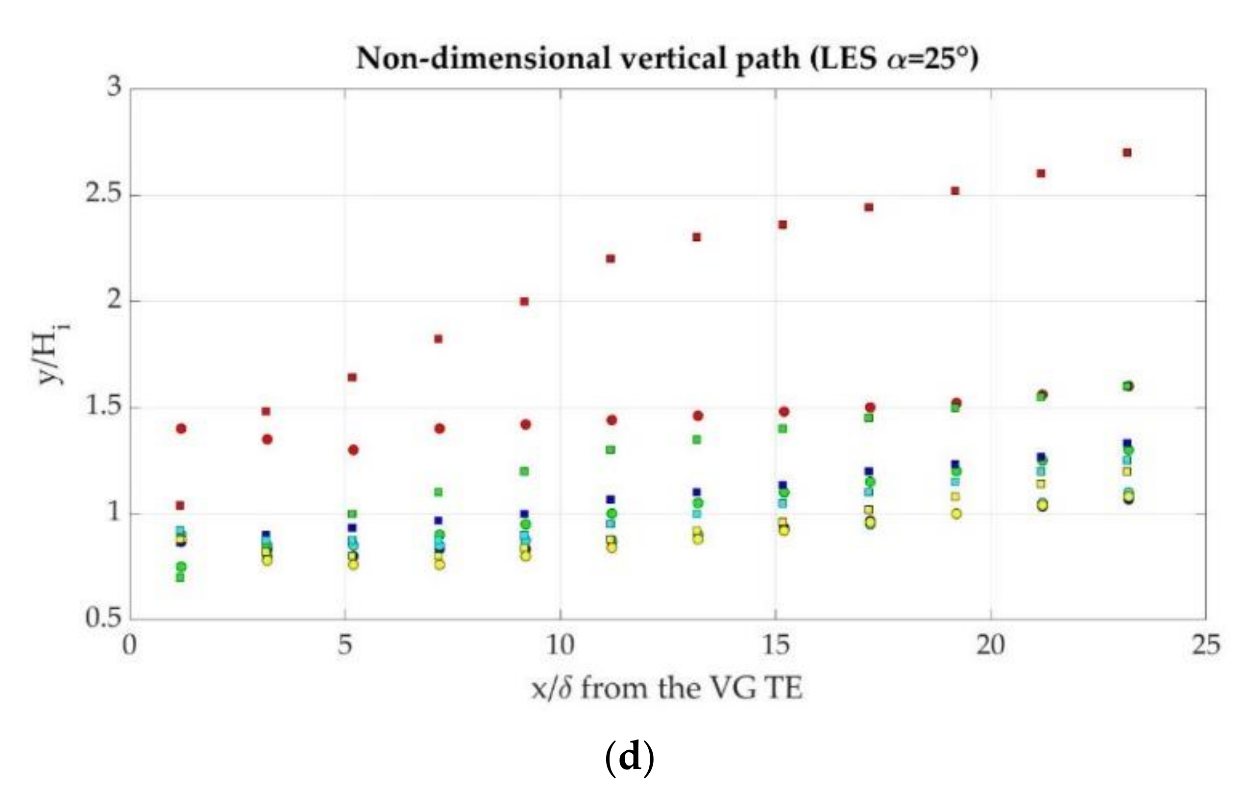
3.3. Vortex Path

In order to analyze the vortex path of the primary vortex, the location of the center of this vortex is studied. According to Yao et al. [39], the vortex center is the point in where the peak vorticity appears. Figure 10 shows the vertical and lateral path of the primary vortex normalized with the height of each VG. The lateral path obtained in the present study for α = 18° is compared to the one obtained experimentally by Bray [40].

The lateral path shows that in all the cases, the vortex tends to follow the flow direction, showing a linear trend. With both turbulence models, the lower the height of the VG, the greater the horizontal displacement. Good agreements are obtained with the experimental data reported by Bray [40]. Near the VG, the lateral displacements are nearly equal, except with H = 0.2 δ and α = 18°, but as the flow distances from the VG, the differences between cases increase, most notably with α = 25°.

Corresponding the vertical path, the results show that the vortexes tend to collapse near y/H = 1, except for the case H = 0.2 δ, in which the vortex continues its upward climb as it distances from the VG, this is more noticeable with α = 18° than with α = 25°.

The comparison between the fully resolved mesh model and the cell-set model shows that in both cases, the same trend is followed with both models. With RANS, larger lateral displacements are obtained with the cell-set model, while with LES, the larger lateral displacements are obtained with the fully resolved mesh model. The cell-set model predicts larger vertical displacements with RANS and LES. For the highest VGs, the results are very similar with both models, but as the VG height decreases, the differences between models increase, especially with LES.

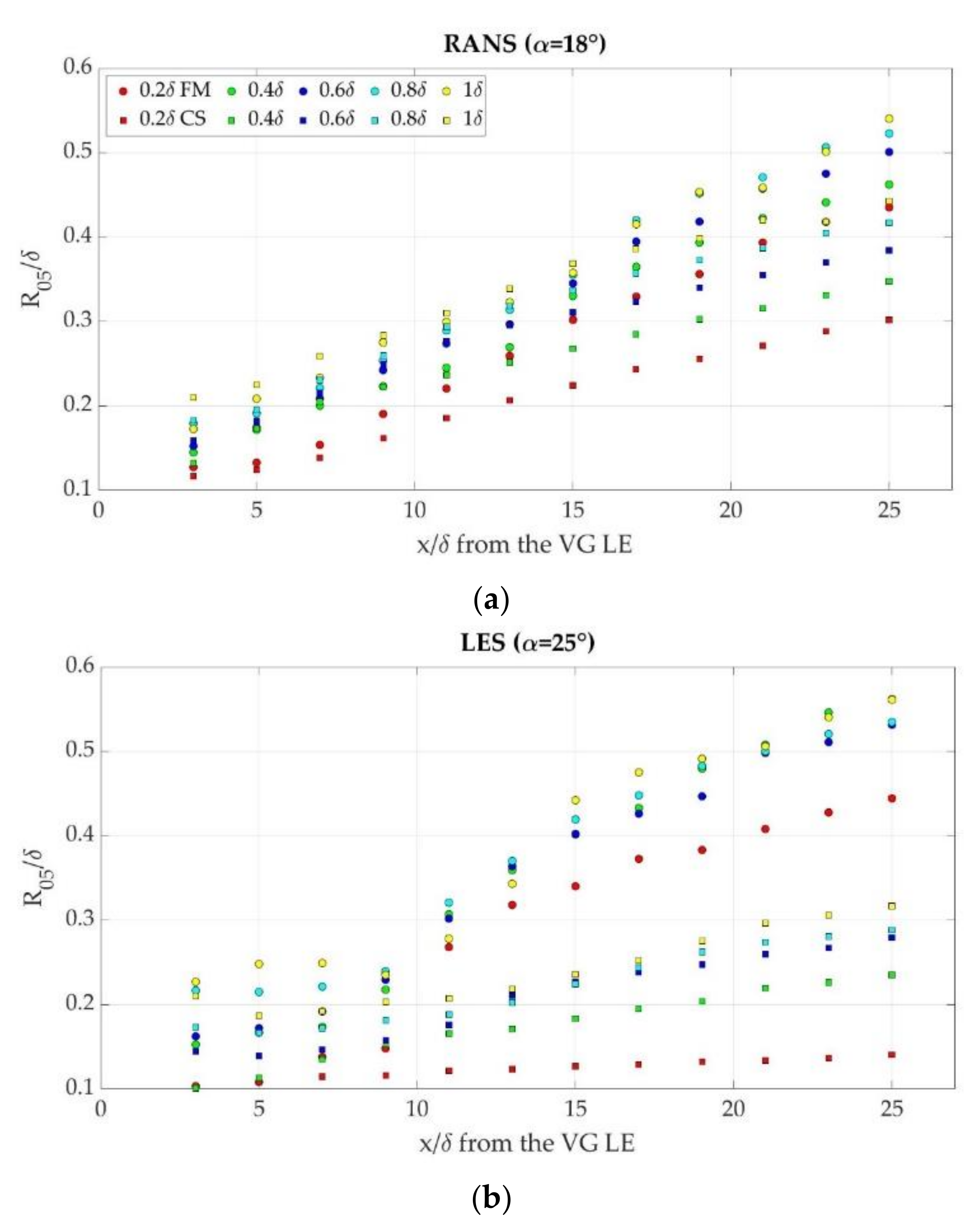
3.4. Vortex Size

The vortex size is analyzed by the Half-Life Radius (R₀₅) parameter developed by Bray [40]. This parameter determines the distance between the vortex center and the point where the local vorticity is equal to $\frac{{\omega }_{peak}}{2}$. As shown in Figure 9, the vortex shape is not always circular, therefore, R₀₅ has been estimated by averaging the values in vertical and lateral directions. Figure 11 shows the R₀₅ values normalized with δ on the wake behind the VG for the tested cases.

The results show that the greatest vortexes appear in the taller VGs. In RANS, the R₀₅ increases linearly from the near-VG region, but in LES, R₀₅ remains almost constant near the VG, and it starts increasing at 10 δ from the VG LE.

Despite showing the same trend, in all the cases, the cell-set model predicts smaller vortexes than the fully resolved mesh model, these differences are more notable with LES. The largest discrepancies between models are visible in the lower VGs, most notably with LES.

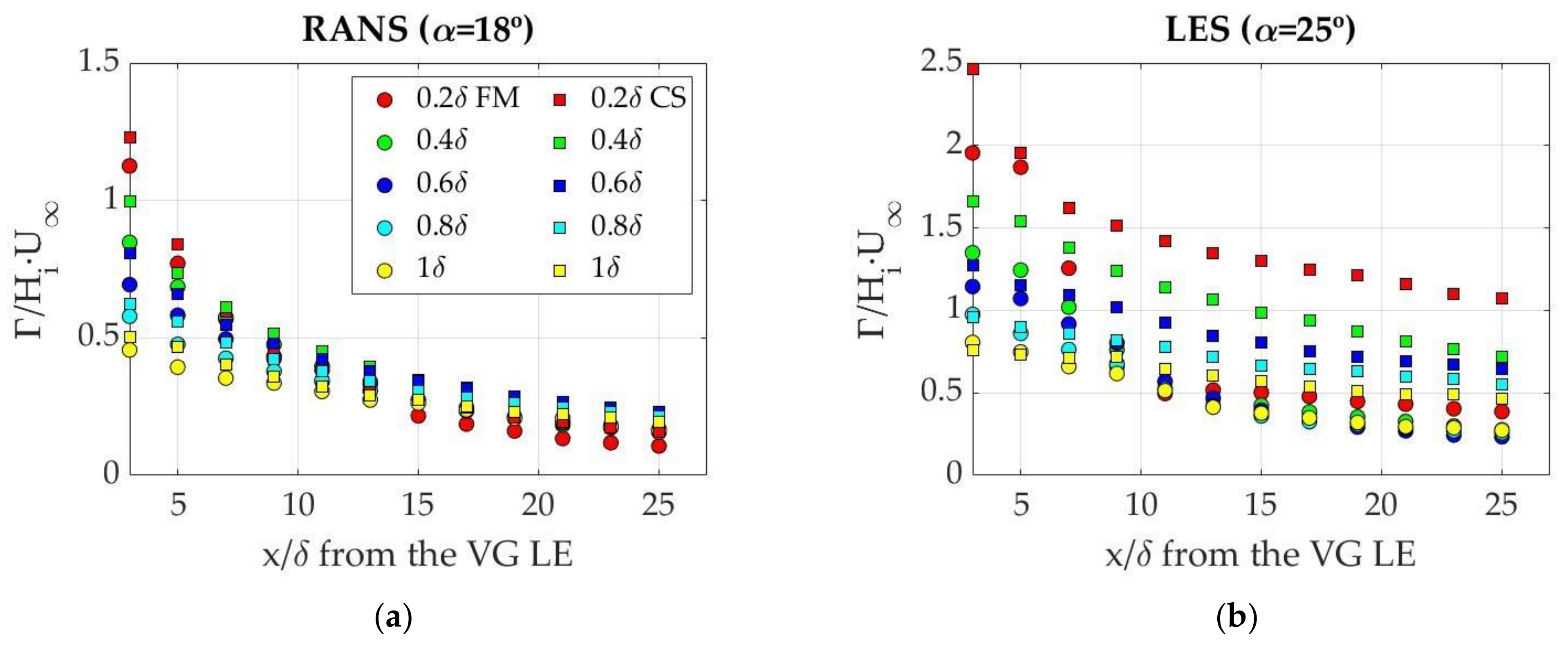
3.5. Vortex Strength

To quantify the vortex strength, vortex circulation (Γ) is considered. This parameter determines the capacity of the vortex to mix the outer flow with the boundary layer [2]. According to Yao et al. [39], the vortex circulation can be estimated by expression (2). Figure 12 shows the vortex circulation normalized with the VG height and the flow streamwise velocity.

$$\Gamma =\frac{{\omega }_{peak}\times \pi \times {R_{05}}^2}{0.693}.$$

(2)

As expected, the vortex losses its strength as it distances from the VG. Close to the VG, the stronger vortices appear in the lower VGs. With RANS, as the distance between the VG and the flow increases, the results tend to collide with both models. In contrast, with LES, this trend is only visible with fully resolved mesh modelling, since with the cell-set model, despite following a falling tendency, the collision of the results is not achieved. With this turbulence model, the normalized circulations are considerably higher with the cell-set model than with the fully resolved mesh model for the lower VGs, but for the higher ones, the differences decrease.

Although, as mentioned before, the R₀₅ values predicted with the fully resolved mesh model are higher, vortex circulation values are very similar with the RANS model. This is attributed to the consideration of the vorticity in the expression of the circulation. With LES, despite showing less differences in Γ than in R₀₅, differences are significant for low VG cases.

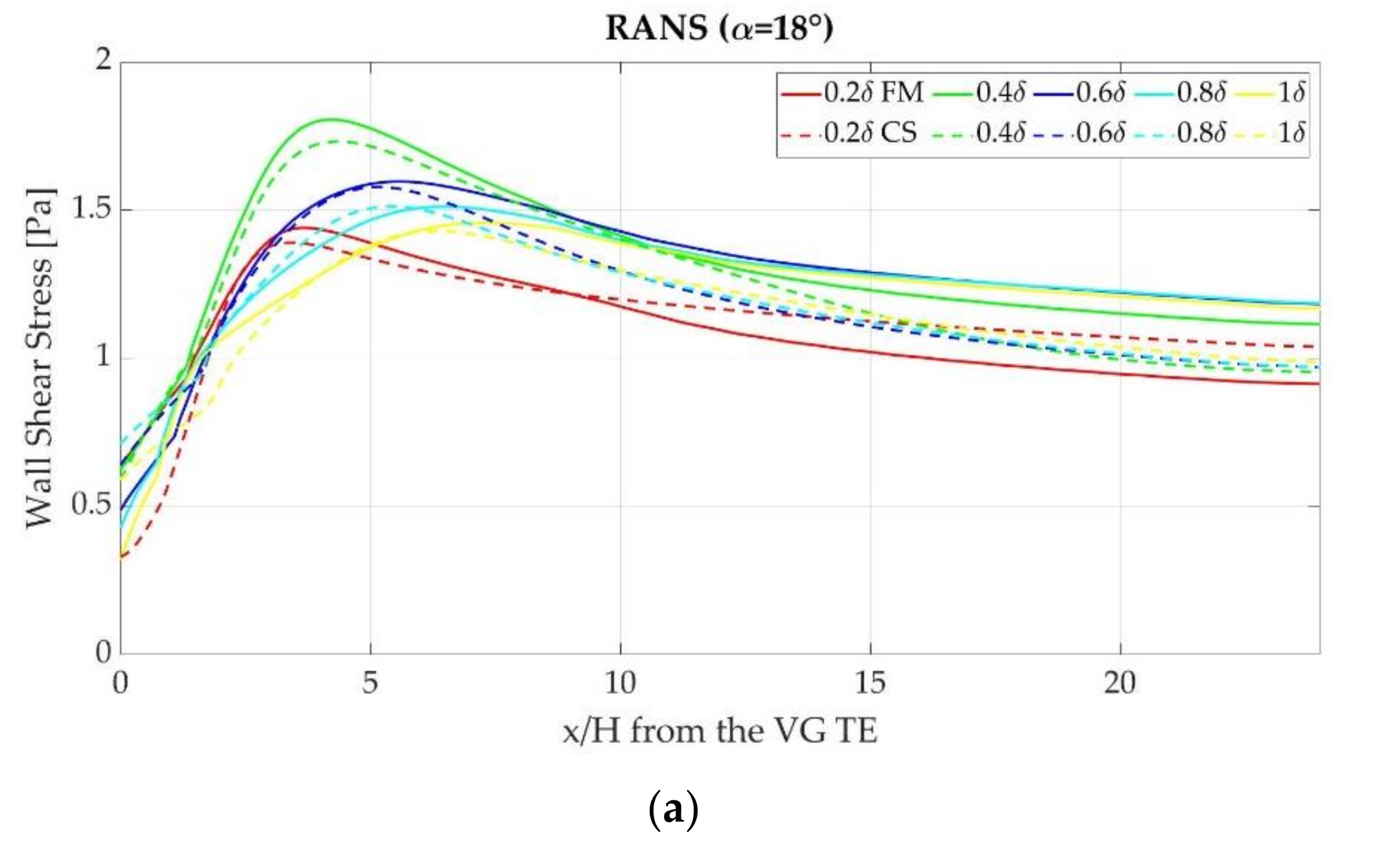
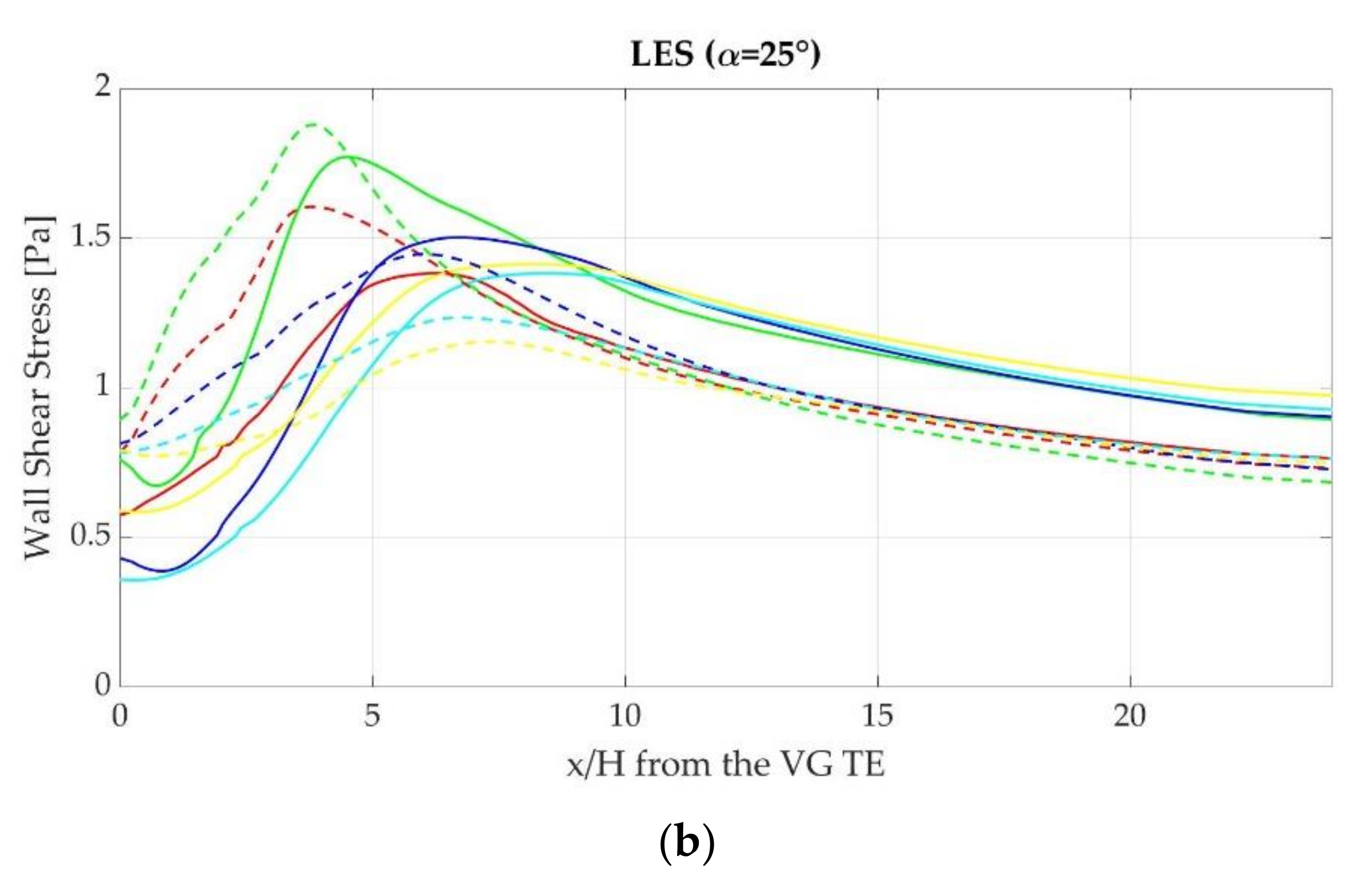
3.6. Wall Shear Stress

Wall shear stress is a major parameter to quantify the capacity of the VG to delay the flow separation. Figure 13 shows the values of the wall shear stress on the wake behind the VG for all the tested cases.

In the tested cases, the wall shear stress goes from a low value to a maximum value, which appears between x/δ = 3 and x/δ = 6, depending on the case. The lower the VG, the closer to the VG the maximum appears. Then, as expected, wall shear stress slightly decreases as it distances from the VG.

According to Godard and Stanislas [41], the optimum angle for the maximum wall shear stress is around 18°, and the wall shear stress is not very sensitive to the aspect ratio. The obtained results are in accordance to these statements, since the values obtained with α = 18° are greater than the ones obtained with α = 25°, and in the majority of the cases, very similar values are obtained, specially far away from the VG.

With RANS, nearly equal locations of the maximums are obtained with both models. Considering the values, very similar values are obtained with both models, but the biggest deviations between models appear when H = 0.2 δ and H = 0.4 δ. With LES, larger discrepancies between models are visible regarding the locations of the maximums, since the cell-set predicts the maximum closer to the VG. The values of the maximums show that the cell-set underpredicts these values for the taller VGs (H = 0.8 δ and H = 1 δ) and overpredicts the values for the lower VGs (H = 0.2 δ and H = 0.4 δ). Far away from the VG, the cell-set model underpredicts the wall shear stress value for all the cases, except for H = 0.2 δ.

The differences visible on the lower VGs for the LES case are attributed to the fact that these VGs are located on the buffer layer region, where the viscous effects are dominant and the flow is strongly turbulent. In this region, the cell-set seems not to be able to provide accurate predictions of both the viscous and turbulent shear stresses.

4. Conclusions

Numerical simulations of 10 different SBVGs on a flat plate in a negligible streamwise pressure gradient flow conditions were conducted using the fully resolved mesh model and the cell-set model with RANS and LES turbulence models, with the objective of analyzing the accuracy of the cell-set model.

The meshes generated with the fully mesh model are made of around 11.5 million cells, while the meshes generated with the cell-set model are composed of around 7.2 million cells. This fact has resulted in savings of around the 40% in terms of computational time.

This study is mainly focused on analyzing the vortexes generated on the wake behind the VG. Therefore, the vortex structure regimes on the wake behind the VG; the path, size, and strength of the primary vortex; and the wall shear stress behind it have been studied. The results demonstrate that the cell-set model is able to predict the vortexes generated on the wake behind the VG. Regarding the primary vortex, nearly equal values of its path and fairly accurate predictions of its size have been obtained. The vortex size and strength show that the cell-set models overpredict the vorticity of the core of the primary vortex, but underpredicts its size, especially with LES. This is reflected in the large differences that appear in the R₀₅, but close values obtained in Γ and wall shear stress.

The major agreements between models appear in the higher VGs, and the biggest disparities appear in the lower ones. This is attributed to the location of the VGs on the boundary layer, since the lower VGs (H = 0.2 δ) are located on the buffer layer and the higher ones (H = 0.8 δ and H = 1 δ) on the outer region. These discrepancies are more notable in LES.

In conclusion, it has been demonstrated that the cell-set model is suitable for RANS turbulence modelling with all the tested SBVGs. With LES, it is adequate for VGs whose height is around the boundary layer, but for lower VGs, the differences with the fully resolved mesh model are significant. Hence, the cell-set model presented in the current work seems to be not very accurate for vane heights within the buffer layer.

Since the cell-set model represents a great advantage in terms of computational and meshing time savings, additional research is proposed, applying the studied meshing model on VGs with different conditions and geometries, or using it for generating other devices. Furthermore, more investigations should be done in order to improve the accuracy of the cell-set modelled geometries with heights within the buffer layer.

References

1. Ashill, P.; Fulker, J.; Hackett, K. Research at DERA on Sub Boundary Layer Vortex Generators (SBVGs). In Proceedings of the 39th Aerospace Sciences Meeting and Exhibit, Reno, NV, USA, 8–11 January 2001; American Institute of Aeronautics and Astronautics: Reston, VA, USA, 2001. [Google Scholar]
2. Ashill, P.; Fulker, J.; Hackett, K. Studies of Flows Induced by Sub Boundary Layer Vortex Generators (SBVGs). In Proceedings of the 40th AIAA Aerospace Sciences Meeting & Exhibit, Reno, NV, USA, 14–17 January 2002; American Institute of Aeronautics and Astronautics: Reston, VA, USA, 2002. [Google Scholar]
3. Aramendia-Iradi, I.; Fernandez-Gamiz, U.; Sancho-Saiz, J.; Zulueta-Guerrero, E. State of the Art of Active and Passive Flow Control Devices for Wind Turbines. DYNA 2016, 91, 512–516. [Google Scholar] [CrossRef] [Green Version]
4. Aramendia, I.; Fernandez-Gamiz, U.; Ramos-Hernanz, J.A.; Sancho, J.; Lopez-Guede, J.M.; Zulueta, E. Flow Control Devices for Wind Turbines. In Energy Harvesting and Energy Efficiency; Bizon, N., Mahdavi Tabatabaei, N., Blaabjerg, F., Kurt, E., Eds.; Lecture Notes in Energy; Springer: Cham, Switzerland, 2017; Volume 37, pp. 629–655. ISBN 978-3-319-49874-4. [Google Scholar]
5. Lin, J.C. Review of Research on Low-Profile Vortex Generators to Control Boundary-Layer Separation. Prog. Aerosp. Sci. 2002, 38, 389–420. [Google Scholar] [CrossRef]
6. Taylor, H.D. Summary Report on Vortex Generators; Research Department Report No. R-05280-9; Research Department, United Aircraft Corporation: Moscow, Russia, 1947. [Google Scholar]
7. Øye, S. The Effect of Vortex Generators on the Performance of the ELKRAFT 1000 KW Turbine. In Proceedings of the 9. Symposium on Aerodynamics of Wind Turbines, Stockholm, Sweden, 11–12 December 1995. [Google Scholar]
8. Miller, G. Comparative Performance Tests on the Mod-2, 2.5-MW Wind Turbine with and without Vortex Generators; NASA TM: Cleveland, OH, USA, 1984.
9. Heyes, A.L.; Smith, D.A.R. Modification of a Wing Tip Vortex by Vortex Generators. Aerosp. Sci. Technol. 2005, 9, 469–475. [Google Scholar] [CrossRef]
10. Tai, T. Effect of Micro-Vortex Generators on V-22 Aircraft Forward-Flight Aerodynamics. In Proceedings of the 40th AIAA Aerospace Sciences Meeting & Exhibit, Reno, NV, USA, 14–17 January 2002; American Institute of Aeronautics and Astronautics: Reston, VA, USA, 2002. [Google Scholar]
11. Agnew, B.; Tam, I.C.; Shi, X. Optimization of Heat and Mass Exchange. Processes 2020, 8, 314. [Google Scholar] [CrossRef] [Green Version]
12. Joardar, A.; Jacobi, A.M. Heat Transfer Enhancement by Winglet-Type Vortex Generator Arrays in Compact Plain-Fin-and-Tube Heat Exchangers. Int. J. Refrig. 2008, 31, 87–97. [Google Scholar] [CrossRef]
13. Subbiah, G.; Allaudeen, A.S.; Janarthanam, H.; Mani, P.; Gnanamani, S.; Raja, K.S.S.; Raja, T.A. Computational Investigation and Design Optimization of Vortex Generator for a Sport Utility Vehicle Using CFD. AIP Conf. Proc. 2020, 2311, 090001. [Google Scholar] [CrossRef]
14. Yu, C.; Zhang, H.; Zeng, M.; Wang, R.; Gao, B. Numerical Study on Turbulent Heat Transfer Performance of a New Compound Parallel Flow Shell and Tube Heat Exchanger with Longitudinal Vortex Generator. Appl. Therm. Eng. 2020, 164, 114449. [Google Scholar] [CrossRef]
15. Carapau, F.; Janela, J. A One-Dimensional Model for Unsteady Axisymmetric Swirling Motion of a Viscous Fluid in a Variable Radius Straight Circular Tube. Int. J. Eng. Sci. 2013, 72, 107–116. [Google Scholar] [CrossRef]
16. Sheng, T.C.; Sulaiman, S.A.; Kumar, V. One-Dimensional Modeling of Hydrodynamics in a Swirling Fluidized Bed. IJMME 2012, 12, 13–22. [Google Scholar]
17. Ibarra-Udaeta, I.; Errasti, I.; Fernandez-Gamiz, U.; Zulueta, E.; Sancho, J. Computational Characterization of a Rectangular Vortex Generator on a Flat Plate for Different Vane Heights and Angles. Appl. Sci. 2019, 9, 995. [Google Scholar] [CrossRef] [Green Version]
18. Martínez-Filgueira, P.; Fernandez-Gamiz, U.; Zulueta, E.; Errasti, I.; Fernandez-Gauna, B. Parametric Study of Low-Profile Vortex Generators. Int. J. Hydrogen Energy 2017, 42, 17700–17712. [Google Scholar] [CrossRef]
19. Fernandez-Gamiz, U.; Errasti, I.; Gutierrez-Amo, R.; Boyano, A.; Barambones, O. Computational Modelling of Rectangular Sub-Boundary Layer Vortex Generators. Appl. Sci. 2018, 8, 138. [Google Scholar] [CrossRef] [Green Version]
20. Gutierrez-Amo, R.; Fernandez-Gamiz, U.; Errasti, I.; Zulueta, E. Computational Modelling of Three Different Sub-Boundary Layer Vortex Generators on a Flat Plate. Energies 2018, 11, 3107. [Google Scholar] [CrossRef] [Green Version]
21. Ballesteros-Coll, A.; Fernandez-Gamiz, U.; Aramendia, I.; Zulueta, E.; Lopez-Guede, J.M. Computational Methods for Modelling and Optimization of Flow Control Devices. Energies 2020, 13, 3710. [Google Scholar] [CrossRef]
22. Chillon, S.; Uriarte-Uriarte, A.; Aramendia, I.; Martínez-Filgueira, P.; Fernandez-Gamiz, U.; Ibarra-Udaeta, I. JBAY Modeling of Vane-Type Vortex Generators and Study on Airfoil Aerodynamic Performance. Energies 2020, 13, 2423. [Google Scholar] [CrossRef]
23. Fernandez-Gamiz, U.; Réthoré, P.-E.; Sørensen, N.N.; Velte, C.M.; Frederik, Z.; Egusquiza, E. Comparison of Four Different Models of Vortex Generators; European Wind Energy Association (EWEA): Copenhagen, Denmark, 2012. [Google Scholar]
24. Bender, E.E.; Anderson, B.H.; Yagle, P.J. Vortex Generator Modelling for Navier–Stokes Codes. In Proceedings of the 3rd ASME-JSME Joint Fluids Engineering Conference: FEDSM ’99, San Francisco, CA, USA, 18–23 July 1999. ASME Paper FEDSM99-6919. [Google Scholar]
25. Errasti, I.; Fernández-Gamiz, U.; Martínez-Filgueira, P.; Blanco, J.M. Source Term Modelling of Vane-Type Vortex Generators under Adverse Pressure Gradient in OpenFOAM. Energies 2019, 12, 605. [Google Scholar] [CrossRef] [Green Version]
26. Jirasek, A. Vortex-Generator Model and Its Application to Flow Control. J. Aircr. 2005, 42, 1486–1491. [Google Scholar] [CrossRef]
27. Ballesteros-Coll, A.; Fernandez-Gamiz, U.; Aramendia, I.; Zulueta, E.; Ramos-Hernanz, J.A. Cell-Set Modelling for a Microtab Implementation on a DU91W(2)250 Airfoil. Energies 2020, 13, 6723. [Google Scholar] [CrossRef]
28. Ibarra-Udaeta, I.; Portal-Porras, K.; Ballesteros-Coll, A.; Fernandez-Gamiz, U.; Sancho, J. Accuracy of the Cell-Set Model on a Single Vane-Type Vortex Generator in Negligible Streamwise Pressure Gradient Flow with RANS and LES. J. Mar. Sci. Eng. 2020, 8, 982. [Google Scholar] [CrossRef]
29. STAR-CCM+ V2019.1. Available online: https://www.plm.automation.siemens.com/ (accessed on 2 June 2020).
30. Menter, F. Zonal Two Equation K-w Turbulence Models for Aerodynamic Flows. In Proceedings of the 23rd Fluid Dynamics, Plasmadynamics, and Lasers Conference, Orlando, FL, USA, 6–9 July 1993; American Institute of Aeronautics and Astronautics: Reston, VA, USA, 1993. [Google Scholar]
31. Allan, B.; Yao, C.-S.; Lin, J. Numerical Simulations of Vortex Generator Vanes and Jets on a Flat Plate. In Proceedings of the 1st Flow Control Conference, St. Louis, MO, USA, 24–26 June 2002; American Institute of Aeronautics and Astronautics: Reston, VA, USA, 2002. [Google Scholar]
32. Urkiola, A.; Fernandez-Gamiz, U.; Errasti, I.; Zulueta, E. Computational Characterization of the Vortex Generated by a Vortex Generator on a Flat Plate for Different Vane Angles. Aerosp. Sci. Technol. 2017, 65, 18–25. [Google Scholar] [CrossRef]
33. Smagorinsky, J. General Circulation Experiments with the Primitive Equations. Mon. Weather Rev. 1963, 91, 99–164. [Google Scholar] [CrossRef]
34. Richardson, L.F.; Gaunt, J.A. The Deferred Approach to the Limit. Philos. Trans. R. Soc. Lond. Ser. A Contain. Pap. A Math. Phys. Character 1927, 226, 299–361. [Google Scholar] [CrossRef]
35. Kuczaj, A.K.; Komen, E.M.J.; Loginov, M.S. Large-Eddy Simulation Study of Turbulent Mixing in a T-Junction. Nucl. Eng. Des. 2010, 240, 2116–2122. [Google Scholar] [CrossRef] [Green Version]
36. Tennekes, H.; Lumley, J.L. A First Course in Turbulence; MIT Press: Cambridge, MA, USA, 1972; ISBN 978-0-262-20019-6. [Google Scholar]
37. Velte, C.M.; Hansen, M.O.L.; Okulov, V.L. Multiple Vortex Structures in the Wake of a Rectangular Winglet in Ground Effect. Exp. Therm. Fluid Sci. 2016, 72, 31–39. [Google Scholar] [CrossRef] [Green Version]
38. Hunt, J.C.R.; Wray, A.A.; Moin, P. Eddies, Stream, and Convergence Zones in Turbulent Flows; Center for Turbulence Research Report CTR-S88; Center for Turbulence Research: Stanford, CA, USA, 1988; pp. 193–208. [Google Scholar]
39. Yao, C.; Lin, J.; Allen, B. Flowfield Measurement of Device-Induced Embedded Streamwise Vortex on a Flat Plate. In Proceedings of the 1st Flow Control Conference, St. Louis, MO, USA, 24–26 June 2002; American Institute of Aeronautics and Astronautics: Reston, VA, USA, 2002. [Google Scholar]
40. Bray, T.P. A Parametric Study of Vane and Air-Jet Vortex Generators. Ph.D. Thesis, Cranfield University, College of Aeronautics, Bedford, UK, 1998. [Google Scholar]
41. Godard, G.; Stanislas, M. Control of a Decelerating Boundary Layer. Part 1: Optimization of Passive Vortex Generators. Aerosp. Sci. Technol. 2006, 10, 181–191. [Google Scholar] [CrossRef]
Figure 1. (a) Numerical domain (not to scale). (b) Vortex Generator (VG) parameters.
Processes 09 00503 g001
Figure 2. Refined mesh around the VG for H = 1 δ. (a) Top view and (b) side view.
Processes 09 00503 g002aProcesses 09 00503 g002b
Figure 3. Mesh resolution and Taylor length scale on the wake behind the VG at y/δ = 1 for the case H = 1 δ with the fully resolved mesh model.
Processes 09 00503 g003
Figure 4. Sketch of the selected cells when using the cell-set model. (a) Geometry of the VG and (b) cell-set representation.
Processes 09 00503 g004
Figure 5. Cell-set construction of the VG with the cell-set model for α = 18° and H = 1 δ. (a) Top view and (b) side view.
Processes 09 00503 g005
Figure 6. Mesh resolution and Taylor length scale on the wake behind the VG at y/δ = 1 for the case H = 1 δ with the cell-set model.
Processes 09 00503 g006
Figure 7. Vortex mechanisms in the wake behind a VG.
Processes 09 00503 g007
Figure 8. Vortical structures predicted on the wake behind the VG. (a) Reynolds-Averaged Navier-Stokes (RANS) (α = 18°) and (b) Large Eddy Simulation (LES) (α = 25°).
Processes 09 00503 g008aProcesses 09 00503 g008b
Figure 9. Primary vortex represented by the Q-criterion with a value of Q = 2500 s−2. The black squares are the projections of the VG Trailing Edges: (a) RANS Fully Resolved Mesh model (α = 18°), (b) RANS cell-set model (α = 18°), (c) LES fully resolved mesh model (α = 25°), and (d) LES cell-set model (α = 25°).
Processes 09 00503 g009
Figure 10. Non-dimensional path of the primary vortex obtained with the fully resolved mesh model (FM), the cell-set model (CS), and experimentally (EXP). (a) Non-dimensional lateral path with RANS, (b) non-dimensional lateral path with LES, (c) non-dimensional vertical path with RANS, and (d) non-dimensional vertical path with LES.
Processes 09 00503 g010aProcesses 09 00503 g010b
Figure 11. R05 normalized with δ. (a) RANS and (b) LES.
Processes 09 00503 g011
Figure 12. Vortex circulation normalized with the VG height and the flow streamwise velocity. (a) RANS and (b) LES.
Processes 09 00503 g012
Figure 13. Wall shear stress on the wake behind the Trailing Edge (TE) of the VG. (a) RANS and (b) LES.
Processes 09 00503 g013aProcesses 09 00503 g013b