Position Output Adaptive Backstepping Control of Electro-Hydraulic Servo Closed-Pump Control System

Abstract

A nonlinear adaptive backstepping control method was proposed to address the system parameter uncertainty problem in the position control process of an electro-hydraulic servo closed-pump control system. This control strategy fully considers the parameter uncertainty of the nonlinear system and establishes the adaptive rate of the uncertain parameter to adjust the parameter disturbance online in real time, thereby improving the accuracy and robustness of the control system. A pump control system experiment platform was used to verify the feasibility of the controller. The experimental results showed that the proposed control strategy provided a good control effect. The pump control system can be controlled with high precision, with a steady-state control accuracy of ±0.02 mm, which serves as a good foundation for the engineering application and promotion of the pump control system.

1. Introduction

The electro-hydraulic servo control system is vital to hydraulic technology and is one of the basic technical components of modern control engineering [1]. Because of its high load-bearing capacity, dynamics, and precision, it is widely used in manufacturing, national defense, military industry, airspace, and other fields [2,3,4]. On the basis of its operating principle, electro-hydraulic servo technology can be classified into two categories: pump control and valve control. Traditional electro-hydraulic servo technology is primarily based on valve control systems. However, owing to the development of electro-hydraulic servo technology in the manufacturing field, electro-hydraulic servo technology with high response, high precision, high power–weight ratio, high power, and low energy consumption has become the goal pursued in the development of hydraulic integrated equipment [5]. In recent years, variable frequency drive and servo drive technology have been gradually perfected; therefore, electro-hydraulic servo closed-pump control (hereinafter referred to as pump control) technology has been developed considerably. Compared with the traditional electro-hydraulic servo valve control technology, pump control technology can not only effectively solve the inherent defects of the former, but also offers the advantages of energy efficiency, high power–weight ratio, and environmental friendliness [6]. Therefore, it is preferred by engineers and has become a topic of focus in the field of electro-hydraulic servo research and development.

An electro-hydraulic position servo system is a typical uncertain nonlinear system [7] that exhibits many nonlinear characteristics and model uncertainties [8]. At present, to address the problems due to of transient parameter time variation and nonlinear factors [9,10,11,12] in electro-hydraulic position servo system [13,14,15], researchers worldwide primarily adopt feedback linearization [16], sliding mode control [17,18,19,20,21,22,23], adaptive control [24,25,26,27], fuzzy control [28,29], and other technologies. As a systematic and structured design method is adopted in backstepping, uncertainties and unknown parameters can be addressed easily in the system [30]. Backstepping can ensure that the final controller exhibit Lyapunov asymptotic stability; therefore, it has been investigated and applied by many scholars.

Kaddissi et al. [31] used the regression least-squares method to estimate the uncertain parameters of a system online and designed an indirect adaptive backstepping controller based on the estimated output value. The experimental results obtained by using this controller and a non-adaptive backstepping controller were compared. The experimental results showed that the indirect adaptive controller can monitor the expected reference signal with a slight transient behavior after parameter changes. However, non-adaptive controllers cannot keep the system on track, thereby resulting in significant oscillations and instability.

Do et al. [32] proposed an anti-winding design method to improve the performance of a strictly feedback single-input adaptive control system with input saturation to solve excessive parameter adaptation under the condition of system input saturation. The over-adaptation problem under a saturated system input was solved by appropriately modifying the adaptive law of unsaturated system inputs. Finally, the simulation results showed that this method improves the control performance in the presence of input saturation constraints.

Guan et al. [33] proposed a nonlinear adaptive robust controller with an adaptive law for a single-rod electro-hydraulic actuator with unknown nonlinear parameters. They used a specific Lyapunov function and combined the inversion method to design the controller of the entire system and the update law of all unknown parameters. Finally, a comparison of position tracking control experiments proved that the proposed nonlinear adaptive robust control method performed better than the control method without adaptive law.

Ba et al. [12] proposed a pump-controlled electro-hydraulic system integrated model inversion controller based on an integrated model inversion method to address the uncertainty and nonlinearity of a hydraulic actuator system. They used an advanced backstepping technique to compensate for nonlinearities and unknowns. Under various operating conditions, a test bench based on a pump-controlled electro-hydraulic system was used to compare the position tracking of a direct backstepping controller (DBS) and a set proportional integral derivative (PID) controller. The experimental results showed that the designed DBS exhibits high controllability.

Yao et al. [34] proposed an ideal compensation adaptive controller for noise interference caused by actual state feedback in an electro-hydraulic servo system. By considering the uncertainty of the modeling of a mismatched system and the nonlinear load pressure state, they adopted a continuous function to approximate the discontinuous symbolic function and designed a strategy on the basis of the backstepping method to construct the expected value of the intermediate state variable. Finally, their comparative experimental results validated the effectiveness of the proposed control strategy.

To address the parameter uncertainty of a nonlinear system in the position control of a pump control system (such as the oil modulus of elasticity, system leakage efficiency, and load equivalent spring stiffness), we propose in this study an adaptive backstepping control strategy for a pump control hydraulic system based on the backstepping method, and its control performance was verified experimentally.

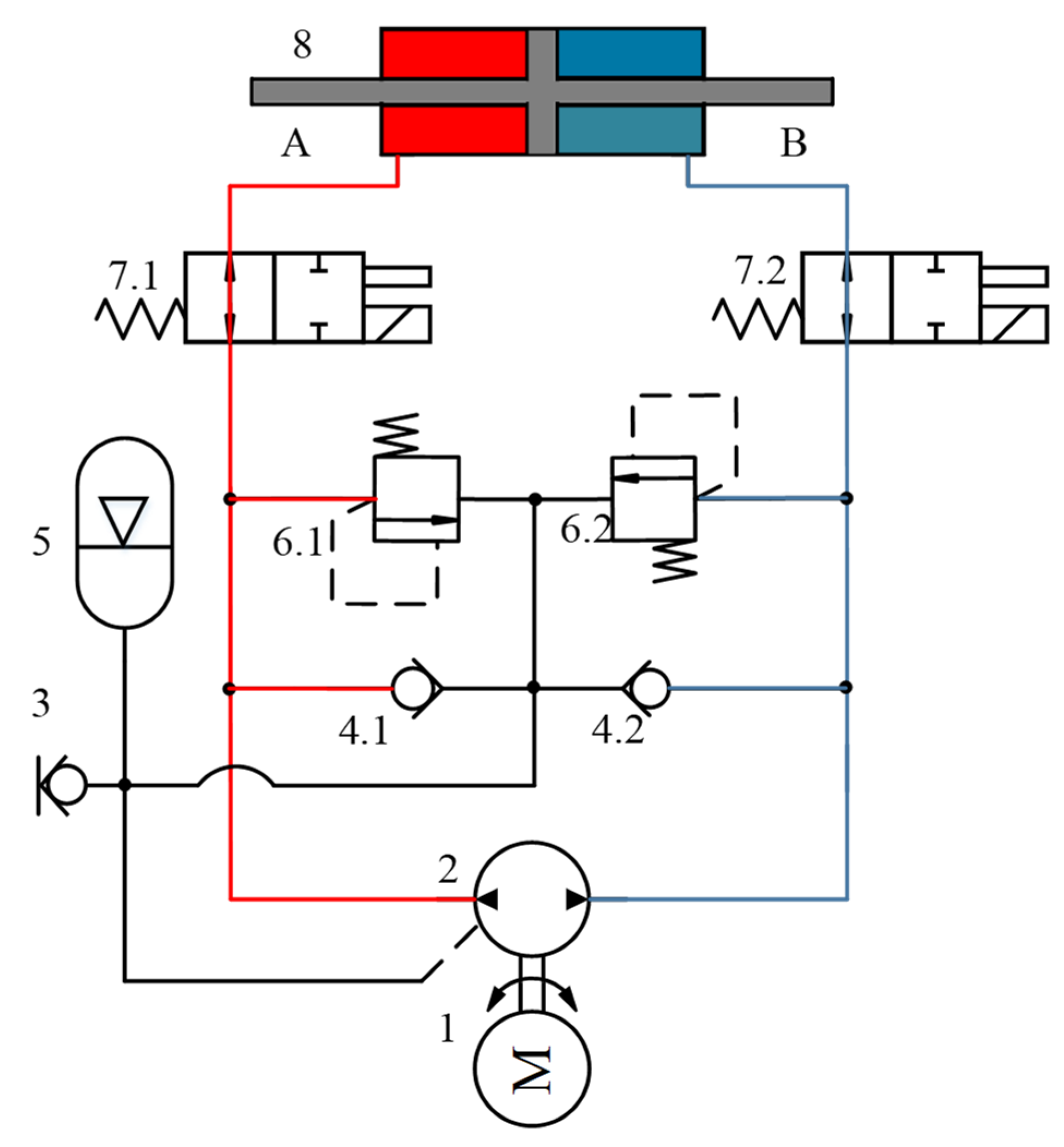
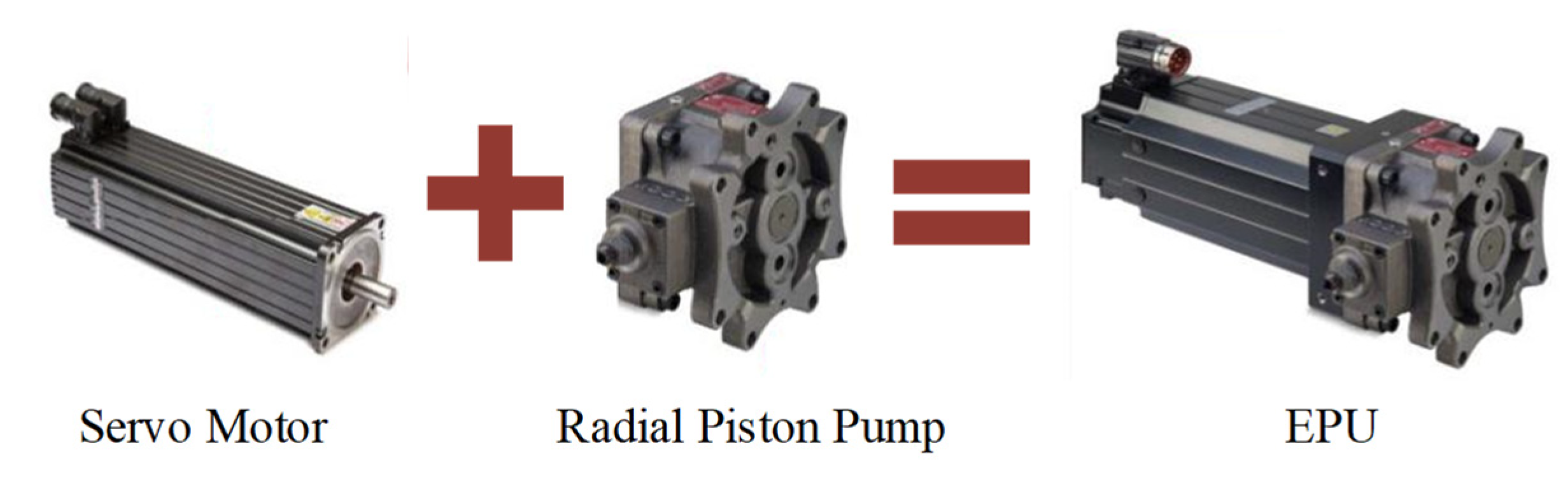
2. Operating Principle of Pump Control System

The structure of the pump control system investigated in this study is shown in Figure 1. The system adopts the integrated volume control scheme of the servo motor and comprises a fixed displacement pump and a hydraulic cylinder. The system has a small equipment volume, simple pipeline layout, no throttle overflow loss, high reliability, high safety, and high precision. In this system, a servo motor is used to drive a fixed displacement pump axially. The inlet port and oil drain of the fixed displacement pump are directly connected to the two load ports of the hydraulic cylinder. The accumulator is combined with a check valve to fill the oil for the system. The relief valve is used as a safety valve to protect the system pressure from exceeding the safety limit value [25]. The controller outputs torque and speed instructions to the servo motor to adjust the output pressure and flow of the fixed displacement pump, thereby enabling the output force and displacement of the hydraulic cylinder piston to be controlled.

The control mode of a pump control system can be typically classified into two categories: variable displacement and variable speed control. The variable speed control mode was adopted in this study to realize the position control of the pump control system by controlling the input voltage of the servo motor to adjust the output speed in real time.

3. Mathematical Model

The mathematical models of the key hydraulic components based on the pump control system are described.

3.1. Servo Motor

The AC servo motor transforms the control input voltage into the motor output speed. As the servo motor has a high response speed and a fast dynamic speed, the relationship between the motor output speed and input control signal is assumed to be a proportional loop, which is expressed as follows:

$${\omega }_p=K_m{u}_c$$

(1)

where ${\omega }_p$ is the output speed of the motor, $K_m$ is the control gain, and $u_c$ is the input voltage signal.

3.2. Fixed Displacement Pump

The flow distribution characteristics of the fixed displacement pump were analyzed considering the oil compression as well as the internal and external leakage. The two-cavity load volume flow from the pump to the controlled hydraulic cylinder can be expressed as follows:

$$\left\{\begin{array}{l}{q}_B=D_p{\omega }_p-C_{ip}(p_A-p_B)+C_{ep}{p}_B\\ q_A=D_p{\omega }_p-C_{ip}(p_A-p_B)-C_{ep}{p}_A\end{array}\right.$$

(2)

where $q_B$ is the flow in cavity B of the system, $q_A$ the flow in cavity A of the system, $p_B$ the pressure in cavity B of the system, $p_A$ the pressure in cavity A of the system, $D_p$ the displacement of the fixed displacement pump, ${\omega }_p$ the input speed of the fixed displacement pump, $C_{ip}$ the internal leakage coefficient of the fixed displacement pump, and $C_{ep}$ the external leakage coefficient of the fixed displacement pump.

3.3. Double-Acting Symmetrical Hydraulic Cylinder

Considering the load condition, oil compression, internal and external leakage, and other factors, we analyzed the flow distribution characteristics of the hydraulic cylinder, and the flow rate continuation equation of the two cavities of the hydraulic cylinder was established as follows:

$$\left\{\begin{array}{l}{q}_A=A_c{\dot{x}}_c+C_{ic}(p_A-p_B)+C_{ec}{p}_A+\frac{V_{cA}}{{\beta }_e}{\dot{p}}_A\\ q_B=A_c{\dot{x}}_c+C_{ic}(p_A-p_B)-C_{ec}{p}_B-\frac{V_{cB}}{{\beta }_e}{\dot{p}}_B\end{array}\right.$$

(3)

where $A_c$ is the efficient working area of the hydraulic cylinder, $x_c$ the displacement of the hydraulic cylinder, ${\beta }_{\mathrm{e}}$ the effective bulk modulus, $V_{cA}$ the compression volume of the hydraulic cylinder’s cavity A, $V_{cB}$ the compression volume of the hydraulic cylinder’s cavity B, $C_{ic}$ the internal leakage coefficient of the hydraulic cylinder, and $C_{ec}$ the external leakage coefficient of the hydraulic cylinder.

The force balance equation of the hydraulic cylinder is as follows:

$$A_c\left(p_A-p_B\right)=m_c{\ddot{x}}_c+B_c{\dot{x}}_c+K{x}_c+\tilde{d}$$

(4)

where $m_c$ is the total mass converted from the load to the piston, $B_c$ the viscous damping coefficient of oil, $K$ the equivalent spring stiffness of the load, and $\tilde{d}$ the external interference and unmodeled friction force.

The block diagram of the closed-pump control system can be established using the Laplace transformation expressed in Equations (1)–(4), as shown in Figure 2. On the basis of the analysis presented in [35], Equation (3) can be simplified as follows:

$${\dot{p}}_A-{\dot{p}}_B=\frac{4{\beta }_e}{V_t}\left[D_p{\omega }_p-A_c{\dot{x}}_c-C_t\left(p_A-p_B\right)\right]$$

(5)

where $V_t$ is the total compression volume.

Substituting the Laplace transformation expressed in Equations (1), (2) and (4) into Equation (5) yields.

$$X_c=\frac{A_c{D}_p{K}_m{u}_c-\left(C_t+\frac{V_t}{4{\beta }_e}s\right)\tilde{d}}{\frac{V_t}{4{\beta }_e}{m}_c{s}^3+\left(\frac{V_t}{4{\beta }_e}{B}_c+C_t{m}_c\right)s^2+\left(\frac{V_t}{4{\beta }_e}K+A_c{}^2+C_t{B}_c\right)s+C_{t}K}$$

(6)

where $C_t=C_{tc}+C_{tp}=C_{ic}+\frac{1}{2}{C}_{ec}+C_{ip}+\frac{1}{2}{C}_{ep}$.

Next, the system state variable $x$ and system output $y$ are defined as follows:

$$\left\{\begin{array}{l}\overrightarrow{x}={\left[x_1,x_2,x_3\right]}^T={\left[x_c,{\dot{x}}_c,\left(p_A-p_B\right)\right]}^T\\ y=x_1\end{array}\right.$$

(7)

On the basis of Equations (1)–(4), the state equation of the pump control system is written as follows:

$$\left\{\begin{array}{l}{\dot{x}}_1=x_2\underset{\underset{}{}}{}\\ {\dot{x}}_2=-\frac{K}{m_c}{x}_1-\frac{B_c}{m_c}{x}_2+\frac{A_c}{m_c}{x}_3+\tilde{d}\\ {\dot{x}}_3=-4\frac{{\beta }_e{A}_c}{V_t}{x}_2-4\frac{{\beta }_e{C}_t}{V_t}{x}_3+4\frac{{\beta }_e{D}_p{K}_m}{V_t}{u}_c\end{array}\right.$$

(8)

Subsequently, the following parameters are defined: ${\theta }_1=K/m_c$, ${\theta }_2=B_c/m_c$, ${\theta }_3=A_c/m_c$, ${\theta }_4=4{\beta }_e{A}_c/V_t$, ${\theta }_5=4{\beta }_e{C}_t/V_t$, and ${\theta }_6=$$4{\beta }_e{D}_p{K}_m/V_t$. Therefore, Equation (8) can be expressed as follows:

$$\left\{\begin{array}{l}{\dot{x}}_1=x_2\\ {\dot{x}}_2=-{\theta }_1{x}_1-{\theta }_2{x}_2+{\theta }_3{x}_3+\tilde{d}\\ {\dot{x}}_3=-{\theta }_4{x}_2-{\theta }_5{x}_3+{\theta }_6{u}_c\end{array}\right.$$

(9)

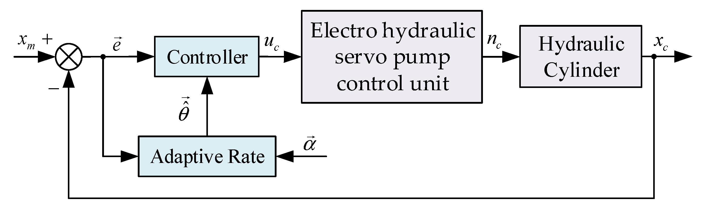
4. Controller Design

On the basis of the effects of the nonlinear and uncertain parameters of the pump-controlled system on the position control, we used the system dynamics model presented in the previous section to design the bounded controller input of the servo motor. Figure 3 shows the control framework of the pump-control system. On the basis of the backstepping criterion, the controller selects the appropriate Lyapunov function and generates the intermediate virtual control variables step by step to obtain the adaptive backstepping controller. The backstepping method ensures that the designed adaptive controller is always Lyapunov asymptotic stable [36].

The controller is designed to achieve $\underset{t\to \infty }{\lim }\left(x_m-x_c\right)=\underset{t\to \infty }{\lim }{e}_1=0$. We assume that the expected trajectory, output speed, acceleration, and acceleration derivative exist and are bounded. The design process of the controller based on backstepping is as follows:

Step 1: Define the position tracking error $e_1$ as

$$e_1=x_1-x_{1d}$$

(10)

where $x_{1d}$ is the expected value of state variable $x_1$. Subsequently, the derivative of $e_1$ with respect to time is as follows:

$${\dot{e}}_1={\dot{x}}_1-{\dot{x}}_{1d}=x_2-{\dot{x}}_{1d}$$

(11)

Next, $e_2$ is defined as the deviation between state variable $x_2$ and its virtual control variable $x_{2d}$.

$$e_2=x_2-x_{2d}$$

(12)

An alternate Lyapunov function is defined as follows:

$$V_1=\frac{1}{2}{e}_1{}^2$$

(13)

Subsequently, the derivative of $V_1$ with respect to time is as follows:

$${\dot{V}}_1=e_1{\dot{e}}_1=e_1\left(e_2+x_{2d}-{\dot{x}}_{1d}\right)$$

(14)

On the basis of Equation (11), when $x_{2d}={\dot{x}}_{1d}-k_1{e}_1-e_2$, the time derivative of $V_1$ is ${\dot{V}}_1=-k_1{e}_1{}^2\le 0$. However, because $e_2$ is the deviation between $x_2$ and $x_{2d}$, $x_{2d}$ cannot contain $e_2$. Hence, $x_{2d}$ is defined as

$$x_{2d}\triangleq {\dot{x}}_{1d}-k_1{e}_1$$

(15)

where $k_1$ is a positive constant. Substituting Equation (15) into Equation (14) yields:

$${\dot{V}}_1=e_1{e}_2-k_1{e}_1{}^2$$

(16)

The aforementioned formula indicates that when $e_2$ is 0, ${\dot{V}}_1$ is negative semidefinite, and the tracking error $e_1$ converges to zero. Therefore, the next task is to design a control law such that the value of $e_2$ approaches zero or is minimized.

Step 2: Take the derivative of $x_{2d}$ with respect to time.

$${\dot{x}}_{2d}={\ddot{x}}_{1d}-k_1\left(x_2-{\dot{x}}_{1d}\right)={\ddot{x}}_{1d}+k_1{\dot{x}}_{1d}-k_1{x}_2$$

(17)

Subsequently, take the derivative of $e_2$ with respect to time.

$${\dot{e}}_2={\dot{x}}_2-{\dot{x}}_{2d}=-{\theta }_1{x}_1-{\theta }_2{x}_2+{\theta }_3{x}_3+\tilde{d}-{\ddot{x}}_{1d}-k_1{\dot{x}}_{1d}+k_1{x}_2$$

(18)

Define the parameter error ${\tilde{\theta }}_i={\widehat{\theta }}_i-{\theta }_i$, where ${\widehat{\theta }}_i$ is an estimate of parameter ${\theta }_i$.

$${\dot{e}}_2=-\left({\widehat{\theta }}_1-{\tilde{\theta }}_1\right)x_1-\left({\widehat{\theta }}_2-{\tilde{\theta }}_2\right)x_2+{\theta }_3{x}_3+\tilde{d}-{\ddot{x}}_{1d}-k_1{\dot{x}}_{1d}+k_1{x}_2$$

(19)

Define a new alternate Lyapunov function as follows:

$$V_2=V_1+\frac{1}{2}{e}_2{}^2+\frac{1}{2{\alpha }_1}{\tilde{\theta }}_1{}^2+\frac{1}{2{\alpha }_2}{\tilde{\theta }}_2{}^2$$

(20)

where ${\alpha }_i$ is the adaptive gain of parameter ${\theta }_i$. Hence, the derivative of $V_2$ with respect to time is expressed as follows:

$$\begin{array}{cc}{\dot{V}}_2& ={\dot{V}}_1+e_2{\dot{e}}_2+\frac{1}{{\alpha }_1}{\tilde{\theta }}_1{\dot{\widehat{\theta }}}_1+\frac{1}{{\alpha }_2}{\tilde{\theta }}_2{\dot{\widehat{\theta }}}_2\hfill \\ & =-k_1{e}_1{}^2+e_2\left[e_1-{\widehat{\theta }}_1{x}_1-{\widehat{\theta }}_2{x}_2+{\theta }_3{x}_3\right.\left.-{\ddot{x}}_{1d}-k_1{\dot{x}}_{1d}+k_1{x}_2\right]\hfill \\ & +e_2\tilde{d}+e_2{\tilde{\theta }}_1{x}_1+e_2{\tilde{\theta }}_2{x}_2+\frac{1}{{\alpha }_1}{\tilde{\theta }}_1{\dot{\widehat{\theta }}}_1+\frac{1}{{\alpha }_2}{\tilde{\theta }}_2{\dot{\widehat{\theta }}}_2\hfill \end{array}$$

(21)

Define $e_3$ as the deviation between state variable $x_3$ and its virtual control variable $x_{3d}$.

$$e_3=x_3-x_{3d}$$

(22)

Similarly, use Equation (21) to design virtual control variable $x_{3d}$.

$$x_{3d}=\frac{1}{{\theta }_3}\left[-k_2{e}_2+{\ddot{x}}_{1d}+k_1{\dot{x}}_{1d}\right.\left.-k_1{x}_2+\widehat{\theta }{x}_1+{\widehat{\theta }}_2{x}_2-e_1\right]$$

(23)

Here, if $k_2>0$, then Equation (21) can be simplified as Equation (23).

$${\dot{V}}_2=-k_1{e}_1{}^2-k_2{e}_2{}^2+{\theta }_3{e}_2{e}_3+e_2\tilde{d}+{\tilde{\theta }}_1\left(e_2{x}_1+\frac{1}{{\alpha }_1}{\dot{\widehat{\theta }}}_1\right)+{\tilde{\theta }}_2\left(e_2{x}_2+\frac{1}{{\alpha }_2}{\dot{\widehat{\theta }}}_2\right)$$

(24)

On the basis of the aforementioned formula, when $e_3$ and $\tilde{d}$ are equal to 0, ${\dot{V}}_2$ is negative semidefinite. Therefore, the next step is to ensure that $e_3$ and $\tilde{d}$ are equal to zero or as small as possible.

Step 3: Because the final control variable $x_3$ is visualized and the control variable $u_c$ exists on its own, virtual control variables are not necessitated in this step.

The derivative of $x_{3d}$ with respect to time can be expressed as

$${\dot{x}}_{3d}=A{\theta }_1+B{\theta }_2+C+D\tilde{d}$$

(25)

where

$$\left\{\begin{array}{cc}A& =\frac{1}{{\theta }_3}\left[k_2{x}_1+k_1{x}_1-{\widehat{\theta }}_2{x}_1\right]\hfill \\ B& =\frac{1}{{\theta }_3}\left[k_2{x}_2+k_1{x}_2-{\widehat{\theta }}_2{x}_2\right]\hfill \\ C& =\frac{1}{{\theta }_3}\left[-k_2\left(k_1{x}_2-{\ddot{x}}_{1d}-k_1{\dot{x}}_{1d}\right)+{\dot{\widehat{\theta }}}_1{x}_1\right.+{\widehat{\theta }}_1{x}_2+{\dot{\widehat{\theta }}}_2{x}_2\hfill \\ & \left.-x_2+{\dot{x}}_{1d}+k_1{\ddot{x}}_{1d}+{\stackrel{⃛}{x}}_{1d}\right]+\left({\widehat{\theta }}_2-k_1\right)x_3-k_2{x}_3\hfill \\ D& =\frac{1}{{\theta }_3}\left[{\widehat{\theta }}_2-k_2-k_1\right]\hfill \end{array}\right.$$

Therefore,

$${\dot{e}}_3={\theta }_6{u}_c-C-D\tilde{d}-A\left({\widehat{\theta }}_1-{\tilde{\theta }}_1\right)-B\left({\widehat{\theta }}_2-{\tilde{\theta }}_2\right)-\left({\widehat{\theta }}_4-{\tilde{\theta }}_4\right)x_2-\left({\widehat{\theta }}_5-{\tilde{\theta }}_5\right)x_3$$

(26)

Next, the Lyapunov function is defined as

$$V_3=V_2+\frac{1}{2}{e}_3{}^2+\frac{1}{2{\alpha }_4}{\tilde{\theta }}_4{}^2+\frac{1}{2{\alpha }_5}{\tilde{\theta }}_5{}^2$$

(27)

Therefore, the derivative of $V_3$ with respect to time is expressed as follows:

$$\begin{array}{cc}{\dot{V}}_3=& -k_1{e}_1{}^2-k_2{e}_2{}^2+e_3\left[{\theta }_3{e}_2-{\widehat{\theta }}_4{x}_2-{\widehat{\theta }}_5{x}_3\right.+{\theta }_6{u}_c-{\widehat{\theta }}_{1}A-{\widehat{\theta }}_{2}B-C\left.-D\tilde{d}\right]\hfill \\ & +e_2\tilde{d}+{\tilde{\theta }}_1\left(e_{3}A+e_2{x}_1+\frac{1}{{\alpha }_1}{\dot{\widehat{\theta }}}_1\right)+{\tilde{\theta }}_2\left(e_{3}B+e_2{x}_2+\frac{1}{{\alpha }_2}{\dot{\widehat{\theta }}}_2\right)\hfill \\ & +{\tilde{\theta }}_4\left(e_3{x}_2+\frac{1}{{\alpha }_4}{\dot{\tilde{\theta }}}_4\right)+{\tilde{\theta }}_5\left(e_3{x}_3+\frac{1}{{\alpha }_5}{\dot{\tilde{\theta }}}_5\right)\hfill \end{array}$$

(28)

The actual control variable $u_c$ can be designed as follows:

$$u_c=\frac{1}{{\theta }_6}\left[-k_3{e}_3-{\theta }_3{e}_2+{\widehat{\theta }}_4{x}_2+{\widehat{\theta }}_5{x}_3\right.+{\widehat{\theta }}_{1}A+{\widehat{\theta }}_{2}B+C+d_{n2}\mathrm{sgn}\left(e_3\right)\left.-\frac{e_2}{e_3}{d}_{n1}\mathrm{sgn}\left(e_2\right)\right]$$

(29)

where $k_3>0$, $d_{n1}\ge \left|\tilde{d}\right|$, and $d_{n2}\ge \left|D\tilde{d}\right|$. Furthermore, the sgn(e) function is defined as follows:

$$\mathrm{sgn}\left(e\right)=\left\{\begin{array}{l}1,\hspace{1em}e>0\\ 0,\hspace{1em}e=0\\ -1,\hspace{1em}e<0\end{array}\right.$$

(30)

On the basis of Equations (28)–(30), the derivative of $V_3$ with respect to time can be expressed as

$$\begin{array}{cc}{\dot{V}}_3& =-k_1{e}_1{}^2-k_2{e}_2{}^2-k_3{e}_3{}^2-e_3\left[D\tilde{d}\right.\left.-d_{n2}\mathrm{sgn}\left(e_3\right)\right]+e_2\left[\tilde{d}-d_{n1}\mathrm{sgn}\left(e_2\right)\right]\hfill \\ & +{\tilde{\theta }}_1\left(e_{3}A+e_2{x}_1+\frac{1}{{\alpha }_1}{\dot{\widehat{\theta }}}_1\right)+{\tilde{\theta }}_2\left(e_{3}B+e_2{x}_2+\frac{1}{{\alpha }_2}{\dot{\widehat{\theta }}}_2\right)\hfill \\ & +{\tilde{\theta }}_4\left(e_3{x}_2+\frac{1}{{\alpha }_4}{\dot{\tilde{\theta }}}_4\right)+{\tilde{\theta }}_5\left(e_3{x}_3+\frac{1}{{\alpha }_5}{\dot{\tilde{\theta }}}_5\right)\hfill \end{array}$$

(31)

The adaptive law of system parameters is expressed as follows:

$$\left\{\begin{array}{l}{\dot{\widehat{\theta }}}_1=-{\alpha }_1\left(e_{3}A+e_2{x}_1\right)\\ {\dot{\widehat{\theta }}}_2=-{\alpha }_2\left(e_{3}B+e_2{x}_2\right)\\ {\dot{\tilde{\theta }}}_4=-{\alpha }_4{e}_3{x}_2\\ {\dot{\tilde{\theta }}}_5=-{\alpha }_5{e}_3{x}_3\end{array}\right.$$

(32)

Therefore, ${\dot{V}}_3$ can be simplified as

$${\dot{V}}_3=-k_1{e}_1{}^2-k_2{e}_2{}^2-k_3{e}_3{}^2-e_3\left[D\tilde{d}-d_{n2}\mathrm{sgn}\left(e_3\right)\right]+e_2\left[\tilde{d}-d_{n1}\mathrm{sgn}\left(e_2\right)\right]\le 0$$

(33)

As shown in Equation (27), the semi-positive Lyapunov function $V_3$ is constructed using Equations (13) and (20), separately. When we adopt Equations (29) and (32) as the input and parameter adaptive law of the system, its derivative ${\dot{V}}_3$ is semi-negative definite. According to Lyapunov stability theory, control errors $e_2$ and $e_3$ are stable at the equilibrium point. According to Barbalat’s lemma, when the state error $e_2$ converges asymptotically to zero, the system output error $e_1$ converges asymptotically to 0 as well.

Therefore, when the pump control system adopts the voltage control rate and the parameter adaptive law, as shown in Equations (29) and (32), the final output position error of the electro-hydraulic servo closed-pump control system will gradually converge to 0.

5. Experimental Results and Analysis

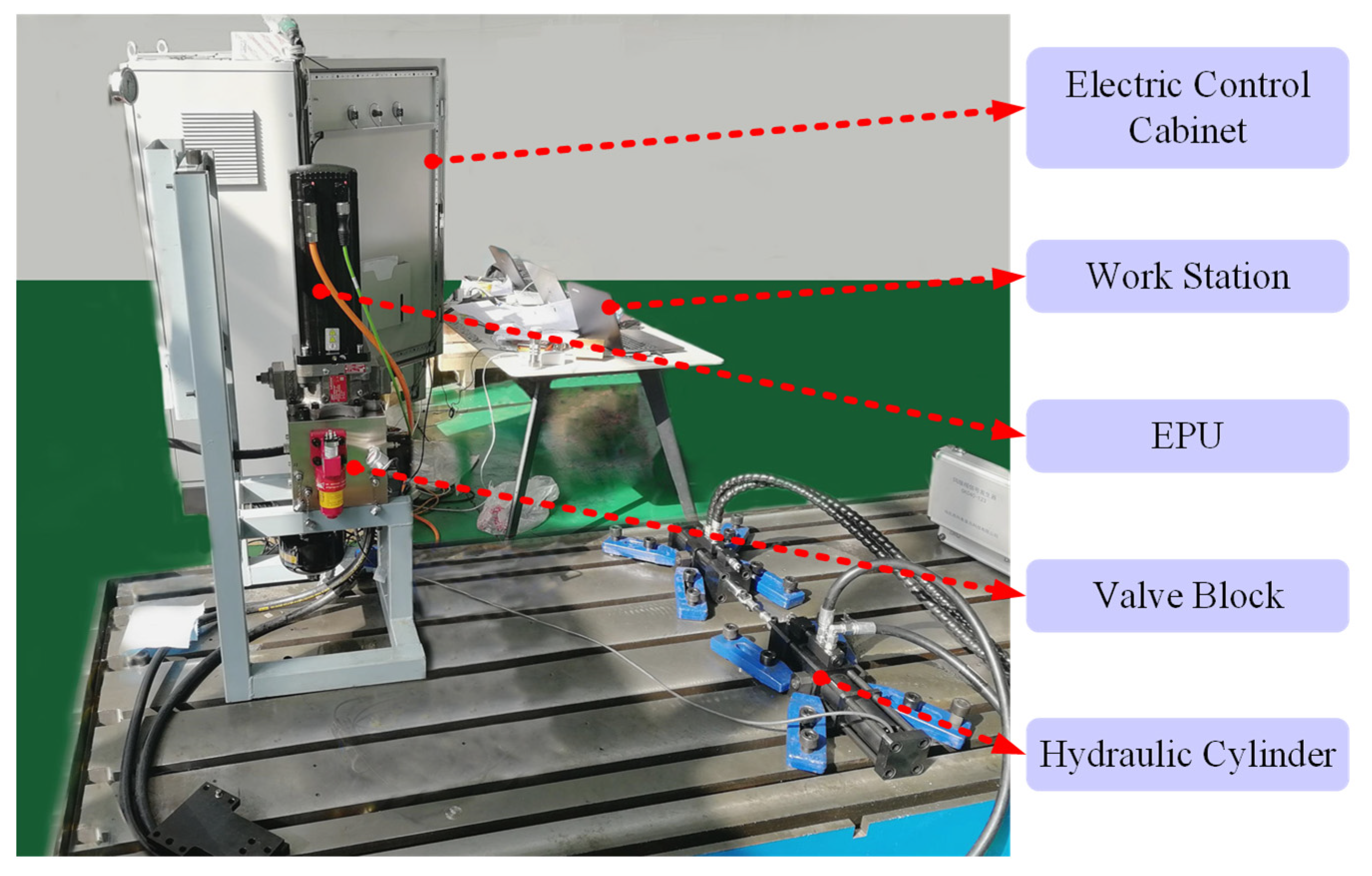
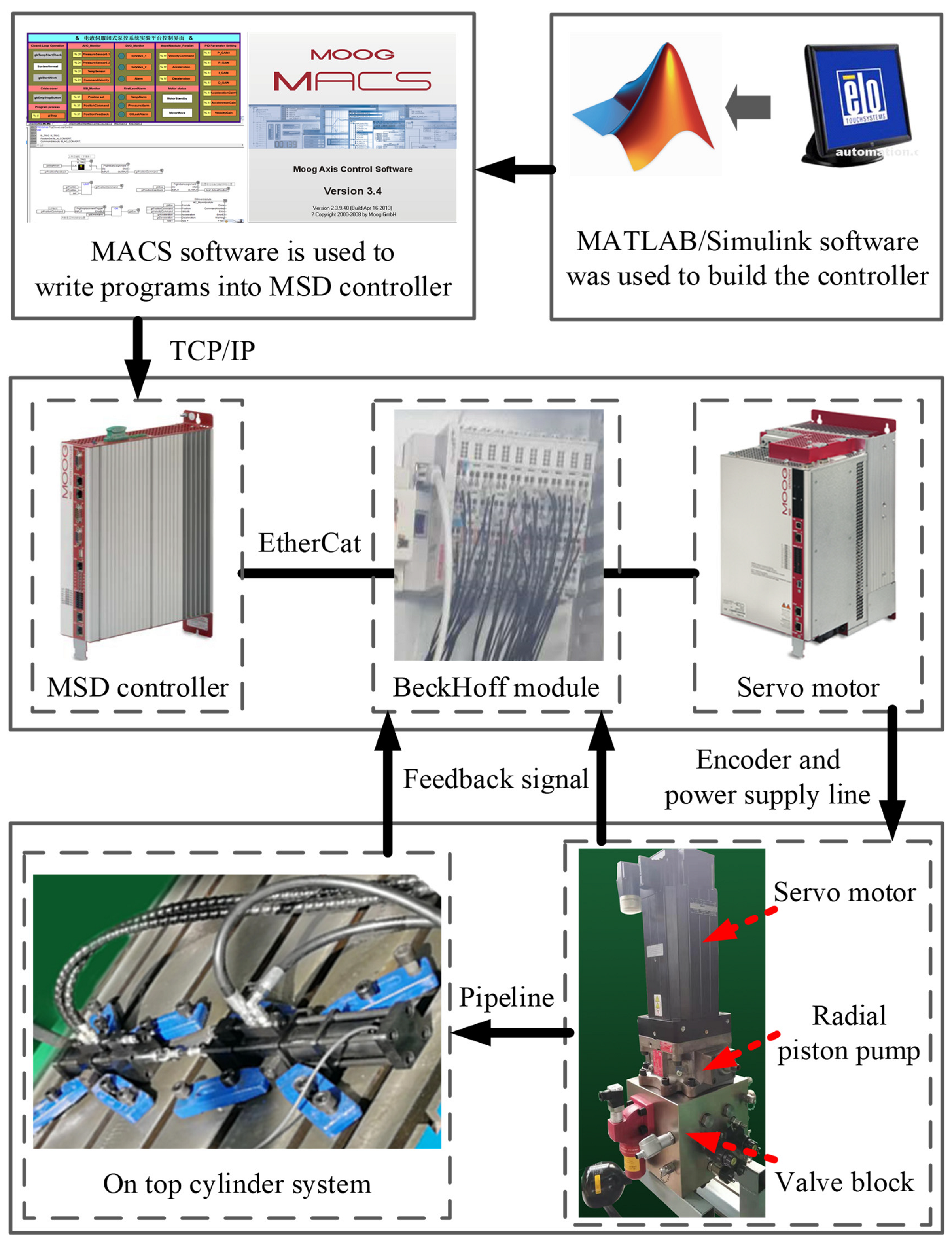
5.1. Experimental Platform

The proposed adaptive backstepping control algorithm was verified experimentally by using the electro-hydraulic servo closed-pump control system experimental platform presented in [37]. Figure 4 shows that the experimental platform is primarily composed of a power unit, a valve block, a hydraulic cylinder, and an electric control cabinet. The working and loading cylinder adopts the structure of the built-in SSI displacement sensor (the sensor model is KH10MB0060MC81S1B10, and the resolution is 1 μm). The power unit adopts an electro-hydraulic servo pump control unit, which is composed of a radial piston pump driven by a permanent magnet synchronous servo motor manufactured by MOOG, referred to as an electro-hydraulic servo pump control unit (herein referred to as EPU). The specific structures are shown in Figure 5.

Figure 6 shows the control structure of the experimental platform. The control software adopts the MOOG axis control software, MACS 3.4. The control hardware is composed of an Advantech IPC-610 computer; Beckhoff modules EK1100, EL3122, and EL2004; a host computer MOOG controller MSD; an MOOG single-axis servo driver; and other auxiliary components. The PC of the device uses MACS 3.4 to write the master control program, imports the MSD of the upper computer through TCP/IP, sends control signals to the servo driver via EtherCat communication, and receives feedback signals from the Beckhoff acquisition module simultaneously.

5.2. Experimental Analysis

The main parameters of the experimental platform are listed in

Table 1. Operating parameters of experimental platform.

Parameter	Symbol	Units	Value
Total compression volume	$V_t$	${\mathrm{m}}^3$	4.15 × 10−2
Efficient working area cylinder	$A_c$	${\mathrm{m}}^2$	7.9 × 10−4
Total mass converted from the load to the piston	$m_c$	$\mathrm{kg}$	150
Viscous damping coefficient	$B_c$	$\mathrm{N}{\left({\mathrm{ms}}^{-1}\right)}^{-1}$	0.0345
Equivalent spring stiffness of the load	$K$	${\mathrm{Nm}}^{-1}$	5 × 107
Total leakage coefficient of hydraulic system	$C_t$	${\mathrm{m}}^3{\left(\mathrm{s}\cdot \mathrm{Pa}\right)}^{-1}$	9 × 10−11
Effective volume modulus of oil	${\beta }_{\mathrm{e}}$	${\mathrm{Nm}}^{-2}$	7 × 108
Control gain	$K_m$	$\left(\mathrm{r}/\min \right)/\mathrm{V}$	300
Displacement of fixed displacement pump	$D_p$	${\mathrm{m}}^3/\mathrm{rad}$	8 × 10−6
External disturbance and unmodeled friction	$d$	$\mathrm{N}$	1.5 × 104

. The adaptive backstepping control algorithm (ABC) was developed using the MATLAB/Simulink software and downloaded to the MOOG MACS axis control software. In this software, the system logic control program was edited to control the position output of the electro-hydraulic servo pump control system. Using the opposite vertex, the cylinder simulated the elastic load of the system, and the expected target signals of the experimental platform were the “S” slope trajectory and sine wave signals, separately. The traditional PID controller and adaptive backstepping controller were used separately to perform the experiment.

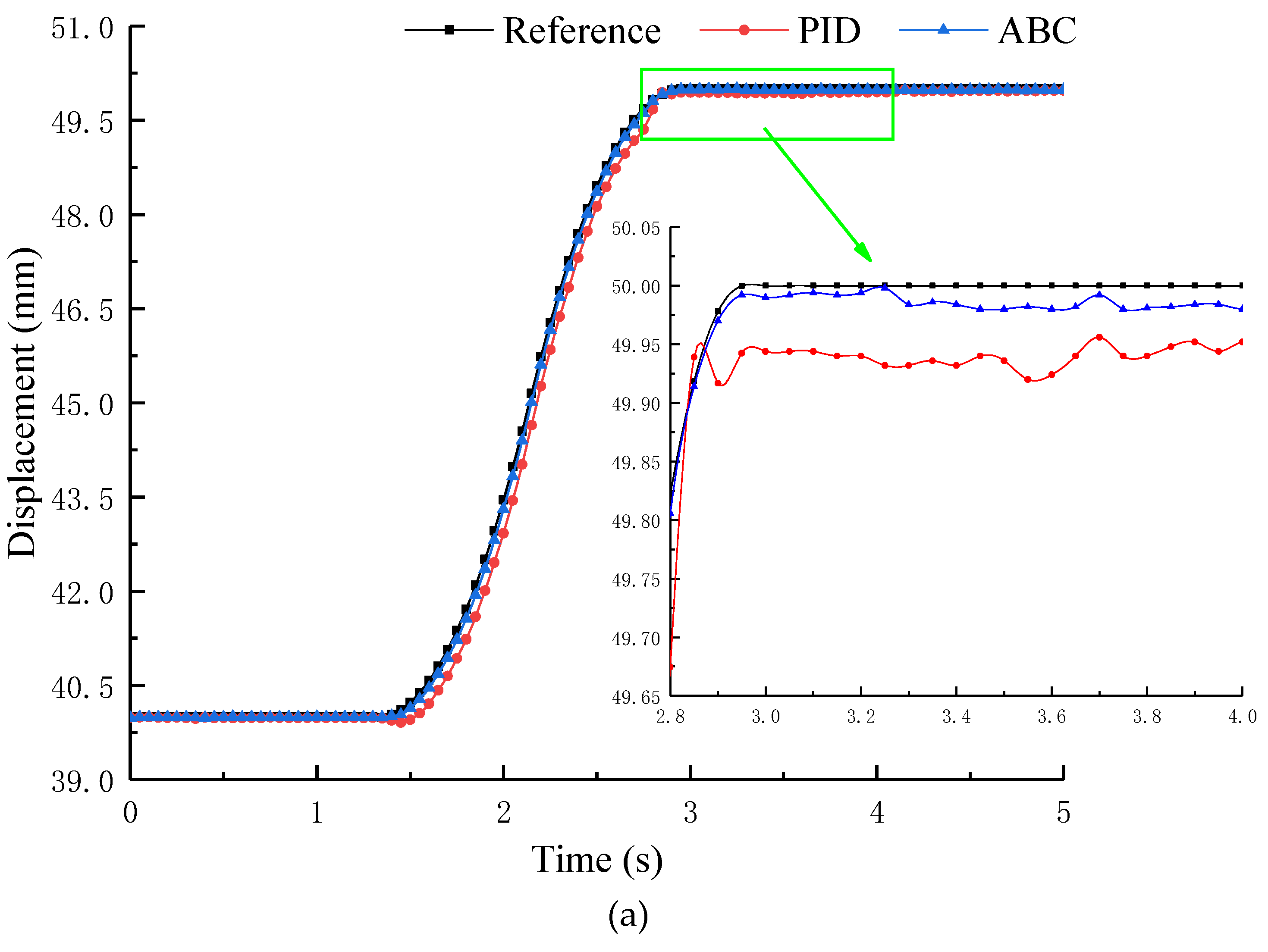
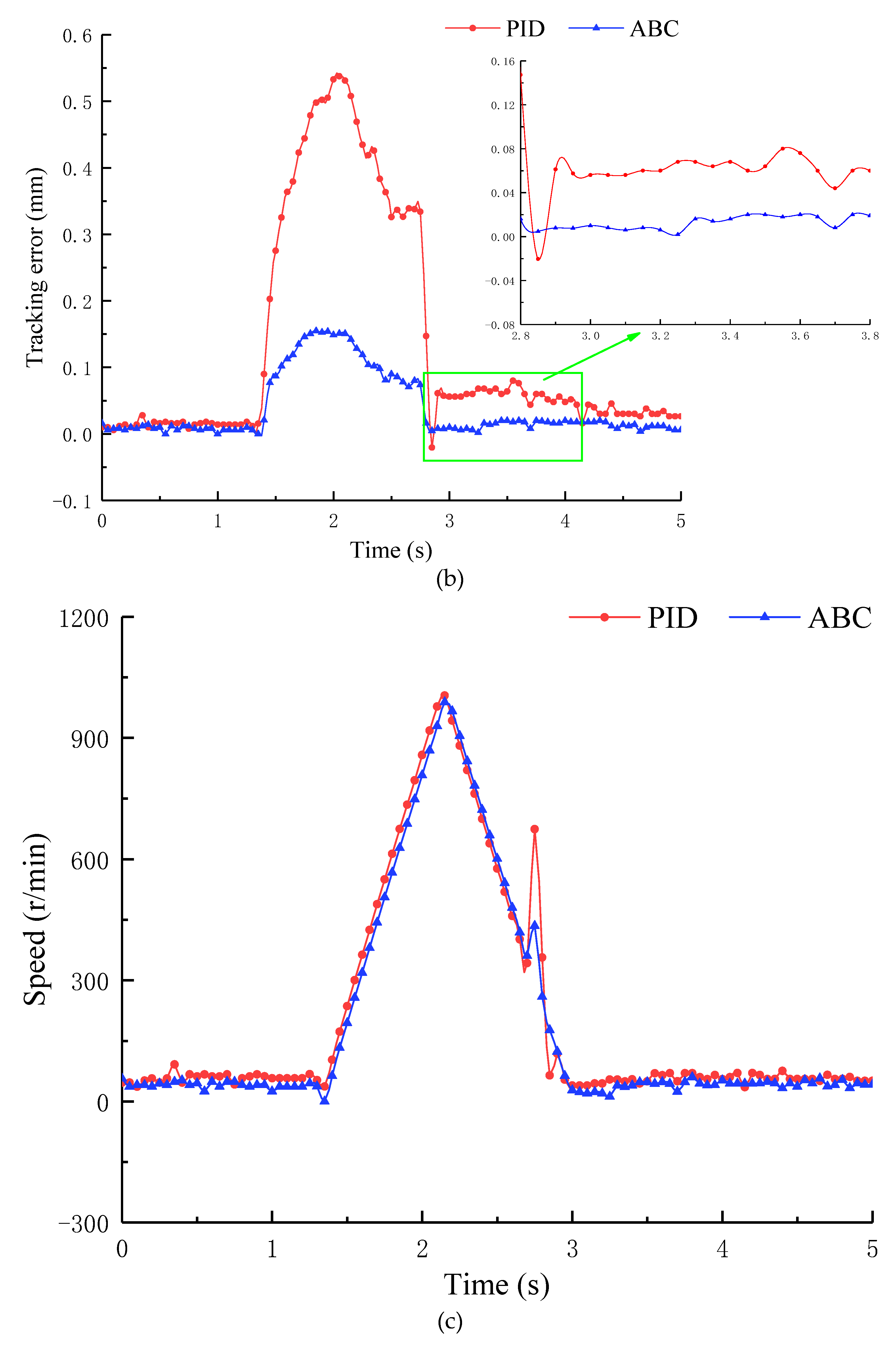
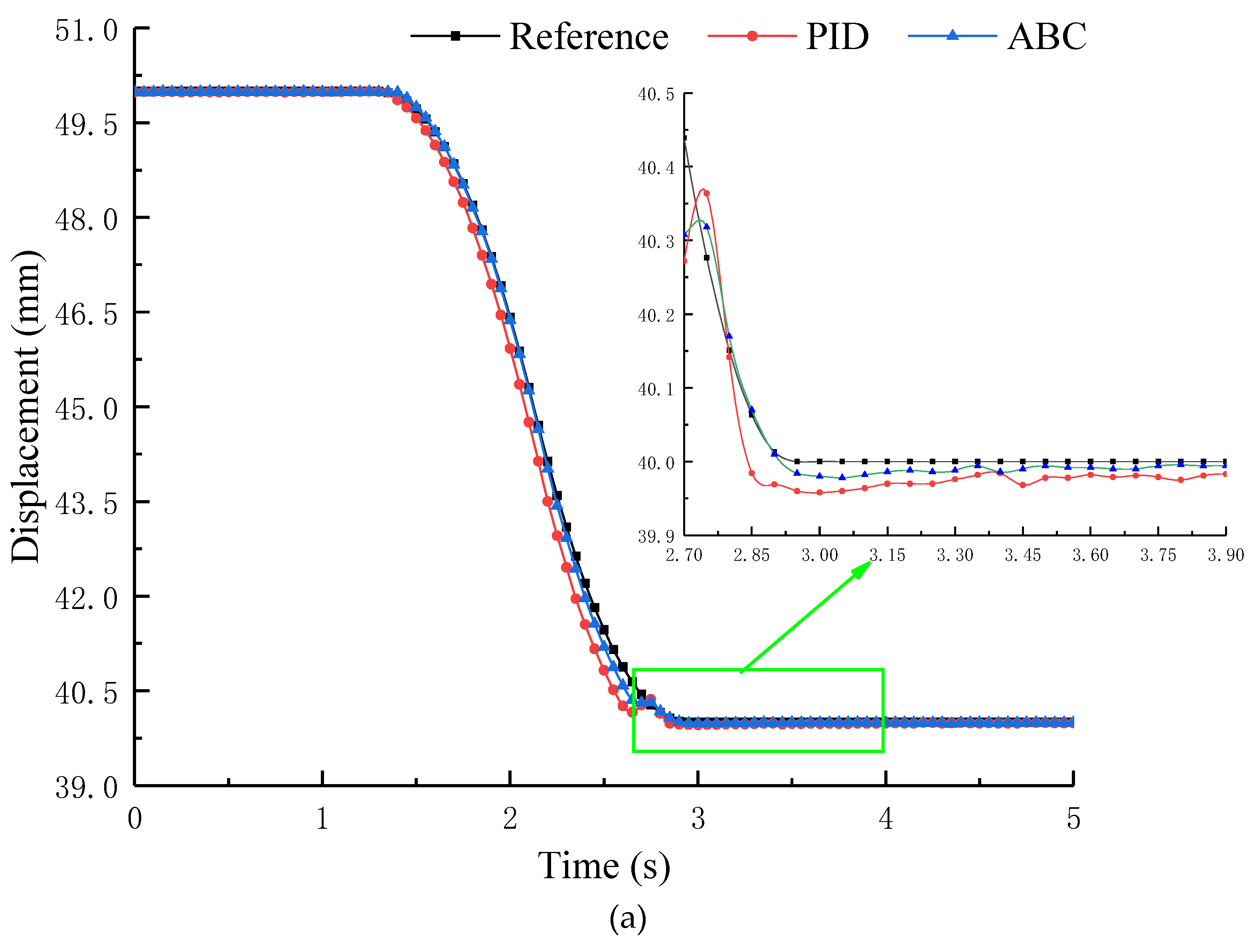
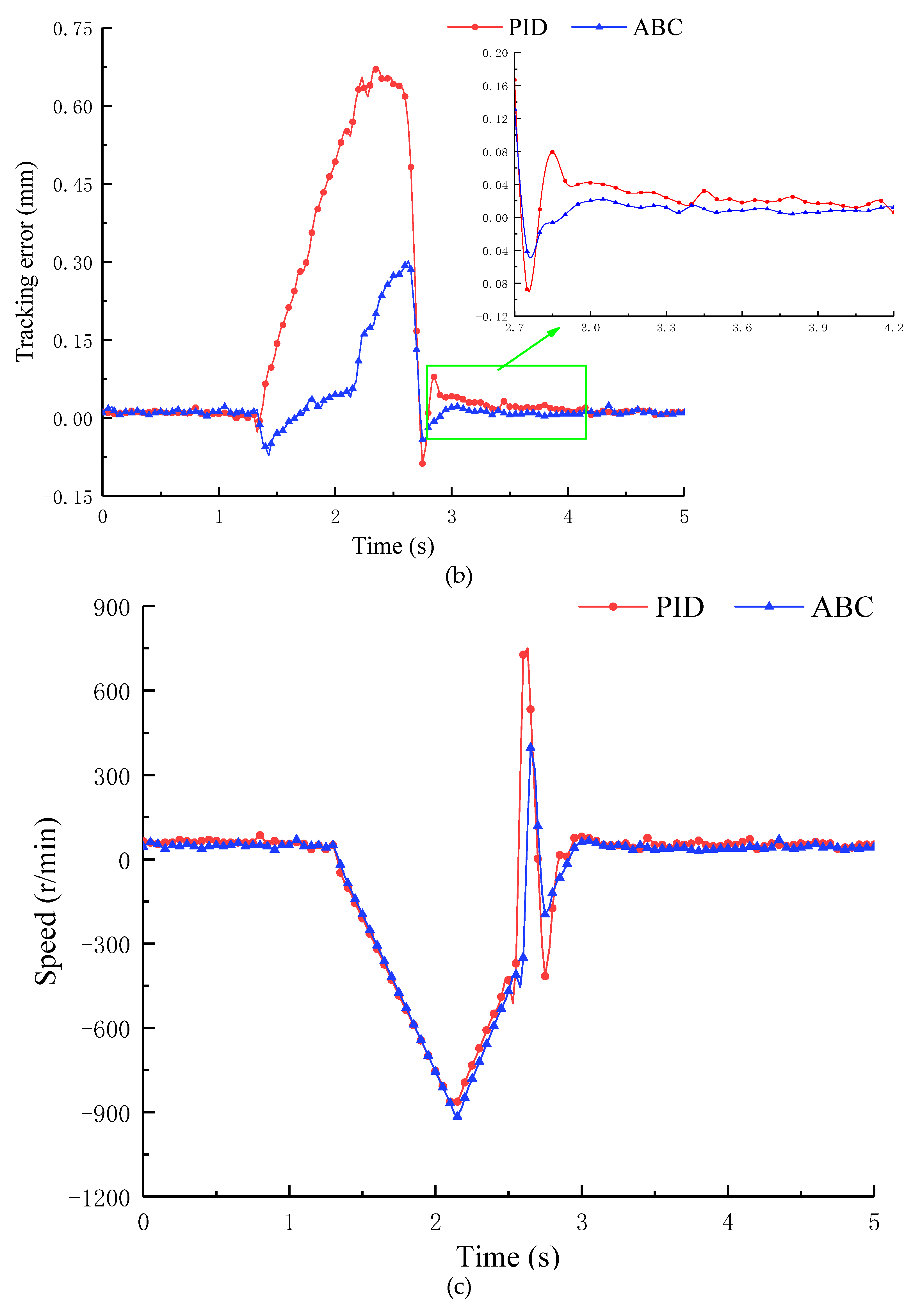
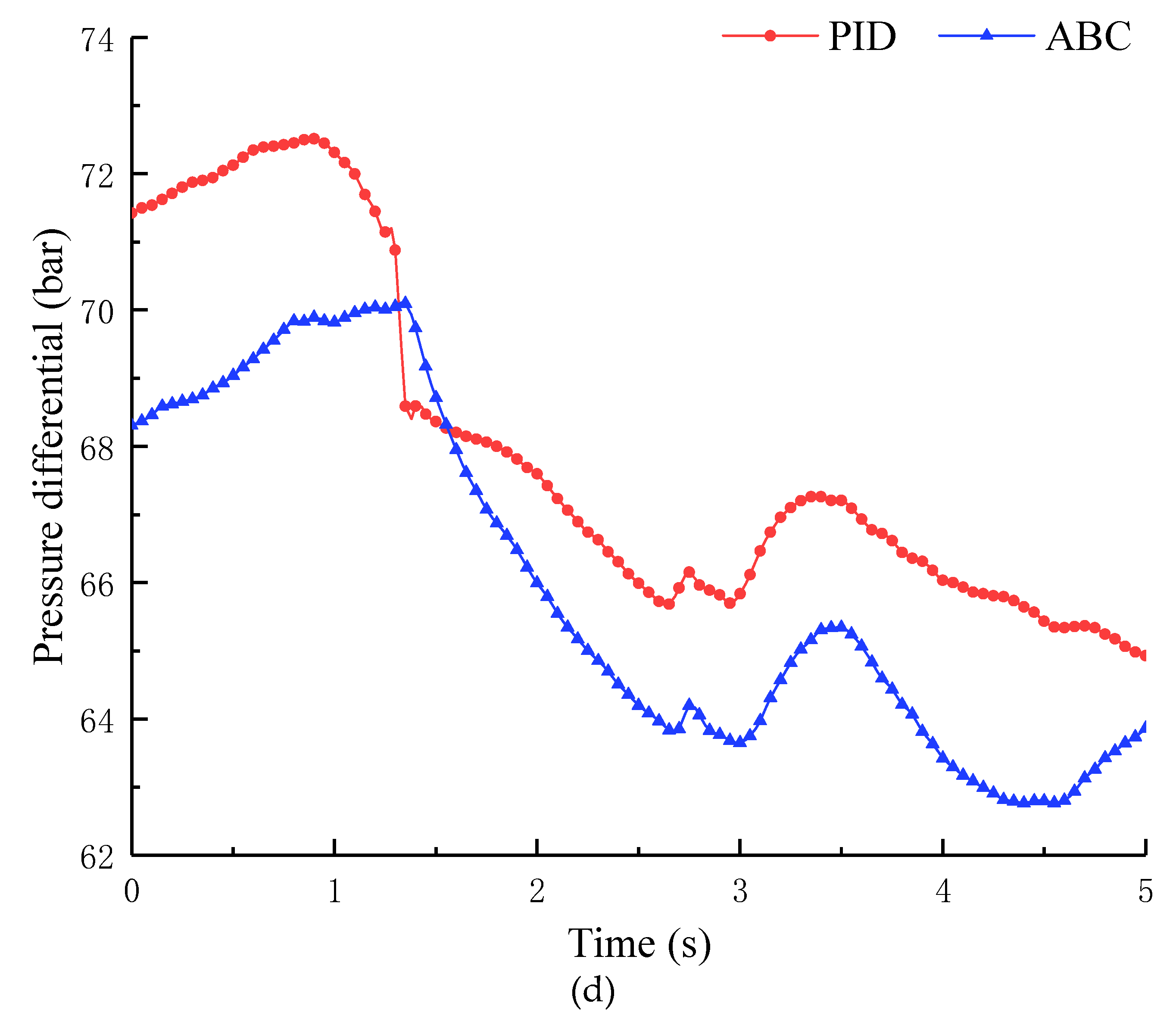
5.2.1. 10 mm “S” Ramp Signal

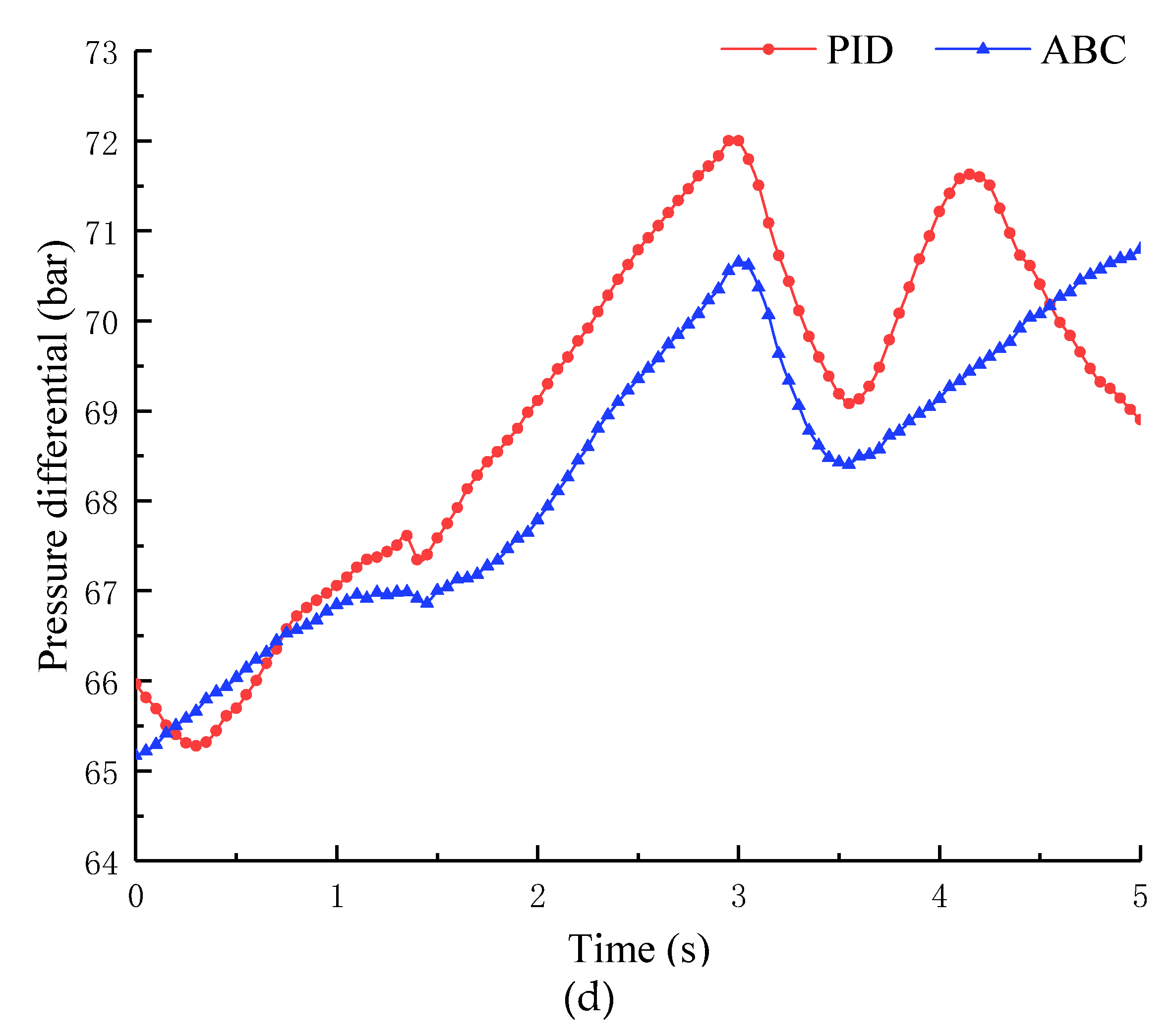
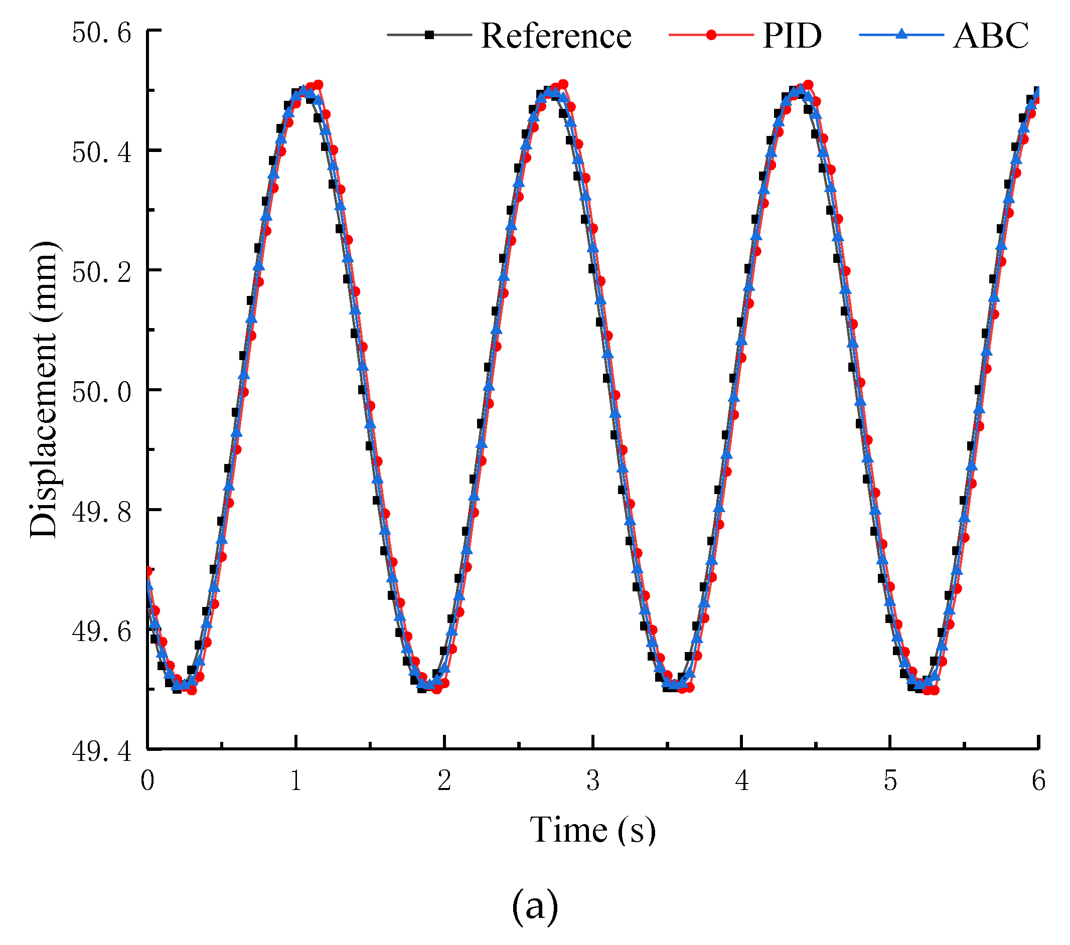
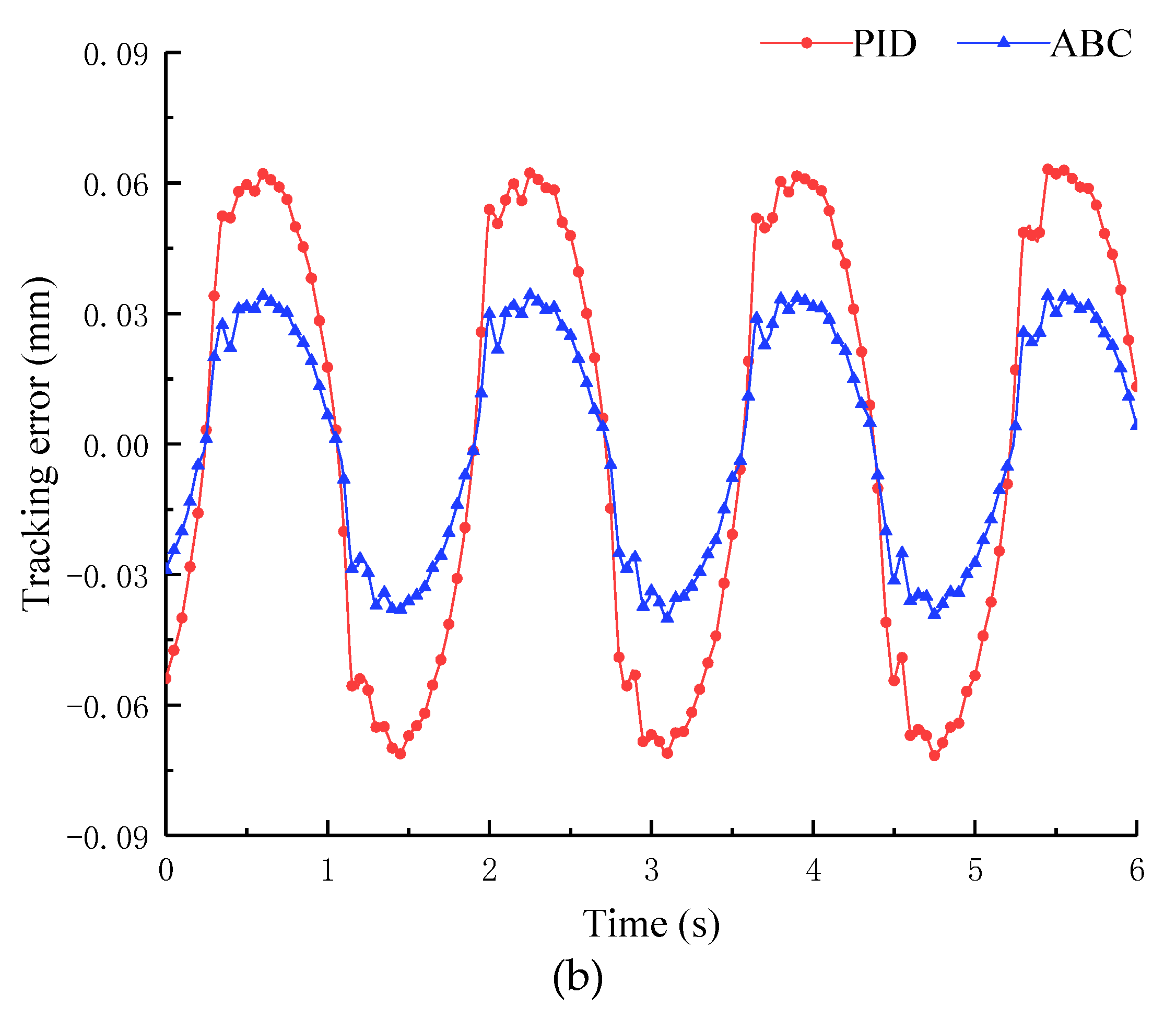
Taking the working load of the pump oil control engine of the thermal power turbine set as an example, we set the load to simulate the output of the hydraulic cylinder of 5 kN and the load fluctuation is ±0.5 kN. By providing an “S”-type ramp signal of 10 mm displacement under the load condition of the system, we obtained the experimental curves of position extension and retraction, as shown in Figure 7 and Figure 8.

Figure 7 shows that the following error of using ABC was much smaller than that of using traditional PID. The steady-state control accuracy of ABC was able to reach ±0.02 mm, while the PID steady-state control accuracy was only ±0.05 mm. Moreover, the time for the system using ABC to reach the steady state was shorter.

As shown in Figure 8, the ABC designed in this paper had better tracking performance than the traditional PID, which is beneficial in terms of alleviating chattering and overshooting in the control process. In addition, the overshoot and the time to reach the steady state of the system using ABC were far less than the time to reach the steady state of the system using PID.

5.2.2. Sine Signal

To further compare and analyze the dynamic characteristics of the traditional PID and ABC, we imposed sine signals with an amplitude of 0.5 mm and a frequency of 0.6 Hz at 50 mm; the experimental results are shown in Figure 9.

As shown in Figure 9, ABC presents better dynamic response characteristics than the traditional PID.

The tracking error of the ABC control was less than ±0.04 mm, and the tracking error of the traditional PID was approximately ±0.06 mm.

The aforementioned experiments indicated that the adaptive backstepping control strategy proposed herein exhibits good control performance in practical engineering applications.

6. Conclusions

Aiming at the position control problem of electro-hydraulic servo closed pump control system, we proposed an adaptive backstepping control strategy. Conclusions are as follows:

(1)

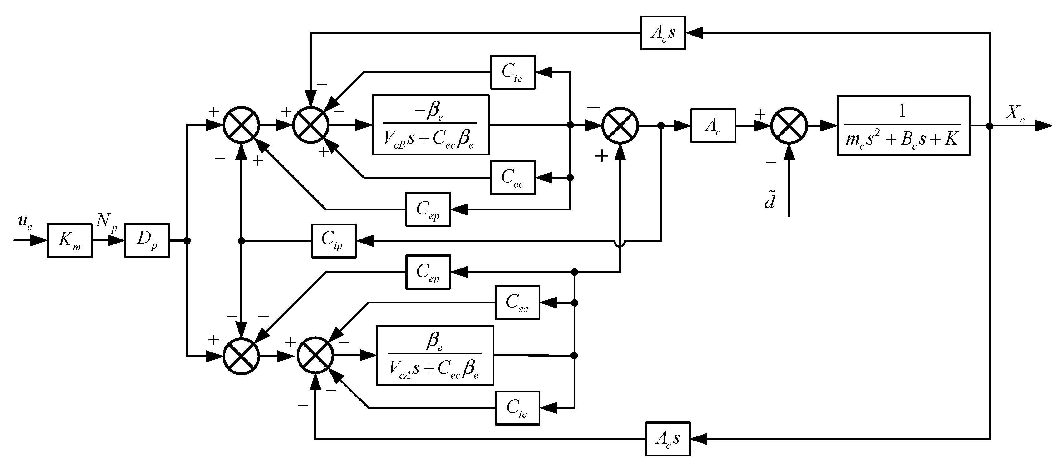
The mathematical model of the electro-hydraulic servo pump control system was established, and the position output transfer function of the system was deduced.

(2)

An adaptive backstepping control strategy was proposed on the basis of the backstepping method. The algorithm fully considers the nonlinearity and parameter uncertainty of the pump control system. When the desired control input is obtained, the adaptive adjustment rate of the uncertain parameter is derived and applied to actual position control.

(3)

Experimental analysis showed that the adaptive backstepping control strategy proposed in this paper had good control performance in practical applications. Its steady-state control accuracy was able to reach ±0.02 mm, which can lay a certain foundation for high-precision position control of the pump control system. In addition, the system dead zone characteristics are also the main factors affecting the steady-state control. In order for the control accuracy of the system to be further improved, the pump control system dead zone characteristics can be further studied.

References

1. Yan, G.; Jin, Z. Research on position control of volume servo electro-hydraulic actuator. J. Xi’an Jiaotong Univ. 2021, 55, 94–100. [Google Scholar]
2. Shao, X.; Zhang, Y.; Sun, G.; Xu, Y. Hydraulicrobot joint force compensation control. J. Electr. Mach. Control 2018, 22, 98. [Google Scholar]
3. Sun, H.; Gao, Q.; Liu, G.; Hou, Y.; Tang, Q. A homologous balance and positioning servo system of fuzzy fractional order PID control. J. Fire Control Command Control 2017, 42, 61–65+71. [Google Scholar]
4. Zuo, X.; Ruan, J.; Sun, J.; Li, S.; Liu, G. Stability analysis of two-dimensional electro-hydraulic servo valve based on extruded oil film theory. J. China Mech. Eng. 2017, 28, 537–543. [Google Scholar]
5. Feng, L.; Yan, H. Nonlinear adaptive robust control of electro-hydraulic servo system. J. Appl. Sci. 2020, 10, 2265–2270. [Google Scholar] [CrossRef]
6. Shen, G.; Zhu, Z.; Zhang, L.; Tang, Y.; Yang, C. Adaptive feed-forward compensation for hybrid control with acceleration time waveform replication on electro-hydraulic shaking table. J. Control Eng. Pract. 2013, 21, 1128–1142. [Google Scholar]
7. Khalil, H.K. Nonlinear Systems; Prentice Hall: Upper Saddle River, NJ, US, 1996. [Google Scholar]
8. Yao, J.; Jiao, Z.; Ma, D.; Yan, L. High-accuracy tracking control of hydraulic rotary actuators with modeling uncertainties. J. IEEE/ASME Trans. Mechatron. 2014, 19, 633–641. [Google Scholar] [CrossRef]
9. Hao, Y.; Xia, L.; Ge, L.; Wang, X.; Quan, L. Research on position control characteristics of hybrid linear drive system. J. Trans. Chin. Soc. Agric. Mach. 2020, 51, 379–385. [Google Scholar]
10. Maghareh, A.; Silva, C.E.; Dyke, S.J. Parametric model of servo-hydraulic actuator coupled with a nonlinear system: Experimental validation. J. Mech. Syst. Signal Process. 2018, 104, 663–672. [Google Scholar] [CrossRef]
11. Jing, H.; Xu, H.; Jiang, J. Dynamic surface disturbance rejection control for electro-hydraulic load simulator. J. Mech. Syst. Signal Process. 2019, 134, 106293.1–106293.14. [Google Scholar] [CrossRef]
12. Ba, D.X.; Ahn, K.K.; Truong, D.Q.; Park, H.G. Integrated model-based backstepping control for an electro-hydraulic system. J. Int. J. Precis. Eng. Manuf. 2016, 17, 565–577. [Google Scholar] [CrossRef]
13. Huang, W.; Quan, L.; Cheng, H.; Ge, L.; Dong, Z. Velocity and position combined control of hydraulic excavator swing system based on handle integral. J. Beijing Inst. Technol. 2020, 40, 193–197. [Google Scholar]
14. Guo, Q.; Zhao, D.; Zhao, X.; Li, Z.; Wu, L. Internal model control in position control of active suspension electro-hydraulic servo actuator. J. Trans. Chin. Soc. Agric. Mach. 2020, 51, 394–404. [Google Scholar]
15. Guo, P.; Li, Y.; Li, J.; Zhang, B.; Wu, X. Design of primary mirror position control system for large aperture telescope. J. Acta Opt. Sin. 2020, 40, 122–128. [Google Scholar]
16. Sani, S.; Chaji, A. Output feedback nonlinear control of double-rod hydraulic actuator using extended Kalman filter. In Proceedings of the IEEE 4th International Conference on Knowledge-Based Engineering and Innovation (KBEI), Tehran, Iran, 22–22 December 2017; pp. 0349–0354. [Google Scholar]
17. Zad, H.S.; Ulasyar, A.; Zohaib, A. Robust Model Predictive position Control of direct drive electro-hydraulic servo system. In Proceedings of the 2016 International Conference on Intelligent Systems Engineering (ICISE), Islamabad, Pakistan, 15–17 January 2016. [Google Scholar]
18. Shi, G.; Zhou, Q.; Wang, S.; Ju, C. High robust control strategy for electro-hydraulic composite steering system in unpilotless mode. J. Trans. Chin. Soc. Agric. Mach. 2019, 50, 395–402. [Google Scholar]
19. Ji, X.; Wang, C.; Chen, S.; Zhang, Z. Sliding mode backstepping control method for valve-controlled electro-hydraulic Position Servo System. J. Cent. South Univ. (Sci. Technol.) 2020, 51, 1518–1525. [Google Scholar]
20. Jia, C.; Wei, J.; Dong, E.; Gao, X.; He, H. A discrete-time sliding mode control method for multi-cylinder hydraulic press. In Proceedings of the IEEE International Conference on Mechatronics and Automation (ICMA), Beijing, China, 13–16 October 2020; pp. 204–205. [Google Scholar]
21. Ji, X.; Wang, C.; Zhang, Z.; Chen, S.; Guo, X. Nonlinear adaptive position control of hydraulic servo system based on sliding mode back-stepping design method. J. Proc. Inst. Mech. Eng. 2021, 235, 0349–0354. [Google Scholar] [CrossRef]
22. Guo, X.; Wang, C.; Liu, H.; Zhang, Z.; Ji, X. Sliding mode control of pump-controlled electro-hydraulic servo system based on extended state observer. J. Beijing Univ. Aeronaut. Astronsutics 2020, 46, 1159–1168. [Google Scholar]
23. Han, S.; Jiao, Z.; Wang, C.; Shang, Y.; Shi, Y. Fractional integral sliding mode nonlinear control of electro-hydraulic flight turntable. J. Beijing Univ. Aeronaut. Astronautics 2014, 40, 1411–1416. [Google Scholar]
24. Shang, X.; Zhou, H.; Yang, H. Research Status of Active Control Method for Fluid Pulsation in Hydraulic System. J. Mech. Eng. 2019, 55, 216–226. [Google Scholar]
25. Helian, B.; Chen, Z.; Yao, B.; Lyu, L.; Li, C. Accurate Motion Control of a Direct-drive Hydraulic System with an Adaptive Nonlinear Pump Flow Compensation. J. IEEE/ASME Trans. Mechatron. 2020, 26, 2593–2603. [Google Scholar] [CrossRef]
26. Tri, N.M.; Nam, D.N.C.; Park, H.G.; Ahn, K.K. Trajectory control of an electro hydraulic actuator using an iterative backstepping control scheme. J. Mechatron. 2015, 29, 96–102. [Google Scholar] [CrossRef]
27. Yin, X.; Zhang, W.; Jiang, Z.; Pan, L. Adaptive robust integral sliding mode pitch angle control of an electro-hydraulic servo pitch system for wind turbine. J. Mech. Syst. Signal Process. 2019, 133, 105704. [Google Scholar] [CrossRef]
28. Liem, D.T.; Truong, D.Q.; Park, H.G.; Ahn, K.K. A Feedforward Neural Network Fuzzy Grey Predictor-based Controller for Force Control of an Electro-hydraulic Actuator. J. Int. J. Precis. Eng. Manuf. 2016, 17, 309–321. [Google Scholar] [CrossRef]
29. Zhu, Y.; Sun, Y.; Chen, G. Simulation Research on Hydraulic Loading System of Wind Turbine Based on Particle Swarm PID Control. In Proceedings of the IEEE Conference on Telecommunications, Optics and Computer Science (TOCS), Shenyang, China, 11–13 December 2020; pp. 385–388. [Google Scholar]
30. Lin, H.; Li, E.; Liang, Z. Adaptive backstepping controller for electro-hydraulic servo system with nonlinear uncertain parameters. J. Control Theory Appl. 2016, 33, 181–188. [Google Scholar]
31. Kaddissi, C.; Kenne, J.P.; Saad, M. Indirect Adaptive Control of an Electrohydraulic Servo System Based on Nonlinear Backstepping. J. IEEE/ASME Trans. Mechatron. 2011, 16, 1171–1177. [Google Scholar] [CrossRef]
32. Do, H.M.; Basar, T.; Choi, J.Y. An anti-windup design for single input adaptive control systems in strict feedback form. In Proceedings of the 2004 American Control Conference, Boston, MA, USA, 30 June–2 July 2004; pp. 2551–2556. [Google Scholar]
33. Guan, C.; Pan, S. Nonlinear adaptive robust control of singlerod electrohydraulic actuator with unknown nonlinear parameters. J. IEEE Trans. Control Syst. Technol. 2008, 16, 434–445. [Google Scholar] [CrossRef]
34. Yao, J.; Deng, W.; Sun, W. Precision Motion Control for Electro-Hydraulic Servo Systems with Noise Alleviation: A Desired Compensation Adaptive Approach. J. IEEE/ASME Trans. Mechatron. 2017, 22, 1859–1868. [Google Scholar] [CrossRef]
35. Wang, C. Hydraulic Control System; Mechanical Industry Press: Beijing, China, 2012; pp. 41–42. [Google Scholar]
36. Zheng, J.; Yao, J. Robust adaptive tracking control of hydraulic actuators with unmodeled dynamics. J. Trans. Inst. Meas. Contro. 2019, 41, 3887–3898. [Google Scholar] [CrossRef]
37. Chen, G.; Liu, H.; Zhao, P.; Yan, G.; Ai, C. Research on Experimental Platform of Electro-hydraulic Servo Closed Pump Control System. J. Mech. Electr. Eng. 2021, 38, 363–367. [Google Scholar]
Figure 1. Schematic diagram of electro-hydraulic servo closed-pump control system. 1: servo motor; 2: hydraulic pump; 3: oil plug; 4.1/4.2: safety valve; 5: accumulator; 6.1/6.2. the relief valve; 7.1/7.2: solenoid directional valve; 8: hydraulic cylinder. A and B represent the two chambers of the oil cylinder respectively.
Processes 09 02209 g001
Figure 2. Block diagram of pump control system.
Processes 09 02209 g002
Figure 3. Control block diagram of pump control system.
Processes 09 02209 g003
Figure 4. Test platform.
Processes 09 02209 g004
Figure 5. Electro hydraulic servo pump control unit.
Processes 09 02209 g005
Figure 6. Pump control test bench control frame.
Processes 09 02209 g006
Figure 7. The 40–50 mm displacement tracking curve. (a) Position trailing; (b) Tracking error; (c) Motor speed; (d) Pressure difference.
Processes 09 02209 g007aProcesses 09 02209 g007bProcesses 09 02209 g007c
Figure 8. The 50–40 mm displacement tracking curve. (a) Position trailing; (b) Tracking error; (c) Motor speed; (d) Pressure difference.
Processes 09 02209 g008aProcesses 09 02209 g008bProcesses 09 02209 g008c
Figure 9. Sinusoidal tracking curve. (a) Position trailing; (b) Tracking error.
Processes 09 02209 g009aProcesses 09 02209 g009b