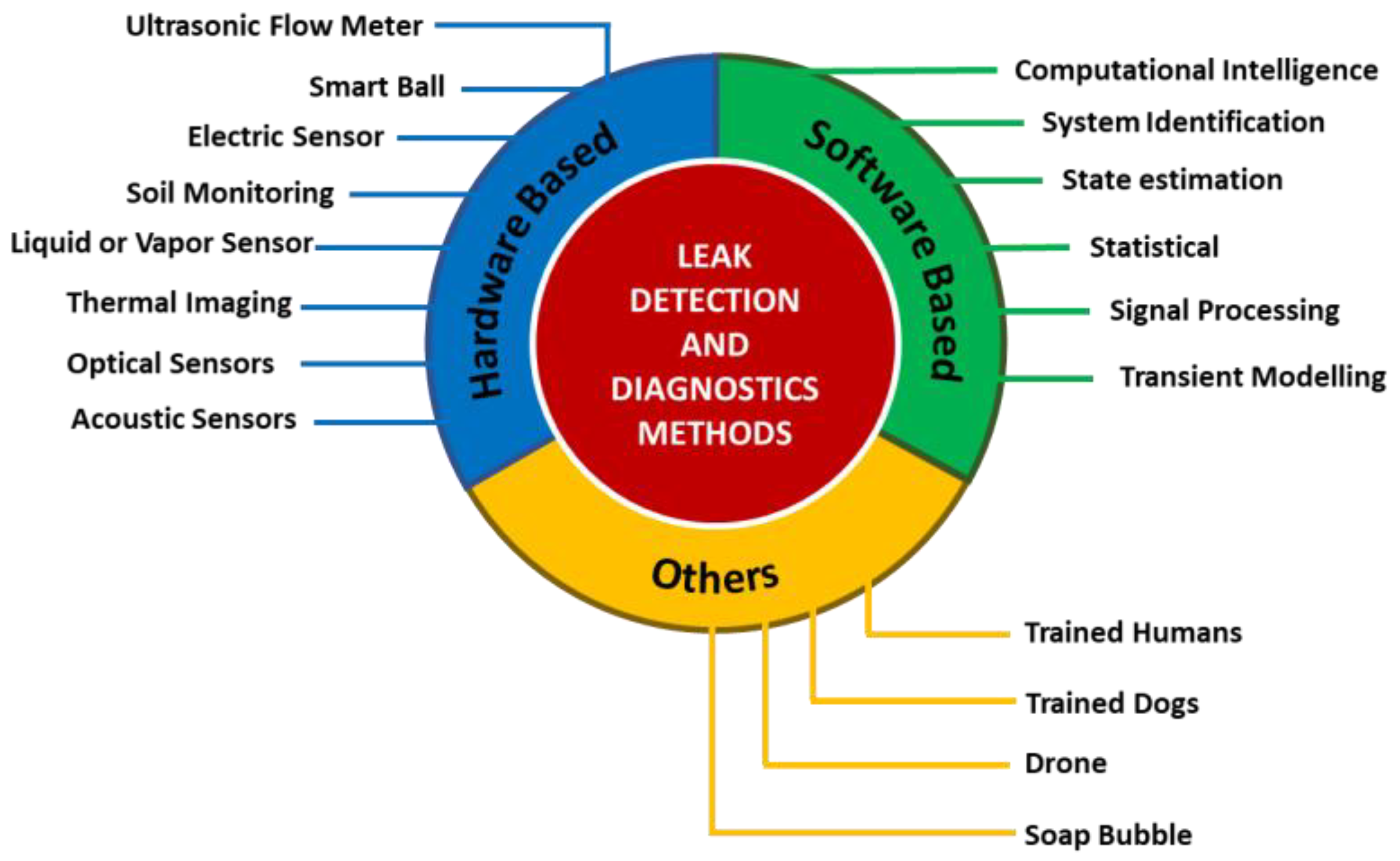
Article

Leak Detection in Gas Mixture Pipelines under Transient Conditions Using Hammerstein Model and Adaptive Thresholds

by
Syed Muhammad Mujtaba
1,
Tamiru Alemu Lemma
1,*,
Syed Ali Ammar Taqvi
2,
Titus Ntow Ofei
3 and
Seshu Kumar Vandrangi
1
1
Department of Mechanical Engineering, Universiti Teknologi PETRONAS, Seri Iskandar 32610, Malaysia
2
Department of Chemical Engineering, NED University of Engineering and Technology, Karachi 75270, Pakistan
3
Department of Geoscience and Petroleum, Norwegian University of Science and Technology, S.P Andersens veg 15a, 7031 Trondheim, Norway
*
Author to whom correspondence should be addressed.
Processes 2020, 8(4), 474; https://doi.org/10.3390/pr8040474
Submission received: 29 February 2020 / Revised: 10 April 2020 / Accepted: 15 April 2020 / Published: 17 April 2020

Abstract

:
Conventional leak detection techniques require improvements to detect small leakage (<10%) in gas mixture pipelines under transient conditions. The current study is aimed to detect leakage in gas mixture pipelines under pseudo-random boundary conditions with a zero percent false alarm rate (FAR). Pressure and mass flow rate signals at the pipeline inlet were used to estimate mass flow rate at the outlet under leak free conditions using Hammerstein model. These signals were further used to define adaptive thresholds to separate leakage from normal conditions. Unlike past studies, this work successfully detected leakage under transient conditions in an 80-km pipeline. The leakage detection performance of the proposed methodology was evaluated for several leak locations, varying leak sizes and, various signal to noise ratios (SNR). Leakage of 0.15 kg/s—3% of the nominal flow—was successfully detected under transient boundary conditions with a F-score of 99.7%. Hence, it can be concluded that the proposed methodology possesses a high potential to avoid false alarms and detect small leaks under transient conditions. In the future, the current methodology may be extended to locate and estimate the leakage point and size.

1. Introduction

Piping systems have been found to be the fastest and economical means to transport oil and gas [1]. Unfortunately, pipelines are not immune to faults such as leakage and blockage, which results in huge losses [2,3]. For instance, in September 2010, San Bruno, California, an old aged gas pipeline exploded due to leakage, resulted in 8 fatalities, 58 injuries and around 14 million-dollar losses [4]. Moreover, leakage in the natural gas pipelines is the largest anthropogenic source of CH4 emission in the USA and the second-largest globally, which significantly contributes to global warming [5]. Therefore, timely and accurate fault detection and diagnostics (FDD) in pipelines is crucial to ensure the safety of human, material, and environment.
According to the comprehensive review by Venkat et al. [6], various FDD techniques have been reported in the previous literature. In Figure 1, an updated (brief) classification of leak detection techniques is presented. Pipeline leak detection techniques can be mainly classified into hardware-based and software-based methods [7,8,9]. Hardware-based methods require the installation of external sensors to monitor signals like acoustic [10], thermal [11] and electric [12], etc. for leak detection in pipelines. Although hardware-based methods have high accuracy, these methods are not cost-effective [13]. While software-based techniques monitor the signals from internally installed sensors for leak detection in pipelines [9]. Soft techniques can be further divided into mechanistic model-based and data-driven techniques. Model-based techniques solve the mathematical models to directly estimate the state of a system [14,15]. Whereas, data-driven FDD techniques are based on measured process input and output signals [16]. While dealing with the highly complex, nonlinear systems that are too difficult to be modeled analytically, data based techniques are preferred [9]. Data-driven techniques can be further divided into statistical, computational intelligence, system identification and, signal processing, etc. as presented in Figure 1. Finally, the conventional techniques, which are also known as biologic methods in which hearing, smelling and watching senses of human beings, animals or machines are used to observe the leaks [8].
Various software-based techniques like fuzzy systems [17] support vector machine [18,19,20,21], neural networks [22,23,24,25], statistical [26,27,28] and, transient models [29,30,31], etc. are applied in faults detection studies. To draw a clear picture of current challenges in pipeline fault detection and diagnostics studies, selected studies are summarized in Table 1. Four critical issues related to leak detection in gas mixture pipelines are highlighted below.
  • Overall, it can be depicted that few studies incorporate pipeline dynamics due to transients in leak detection studies. The studies which considered system transients relied on step transient only [14,31,32]. However, for nonlinear systems, signals should exploit the full range of amplitude and frequency in order to capture all possible system dynamics [33].
  • According to Pan et al. [14], most leak detection studies assume ideal gas conditions; similar observation can be found in Table 1. For instance, Tiantian et al. [31] and Shouxi, Carroll [34] considered gas as an incompressible fluid.
  • From Table 1, it can also be noted that most studies considered small pipelines, i.e., within a length equal to or lesser than 10 km besides, gas pipelines usually have higher lengths [35,36].
  • Effects due to thermal changes is also ignored in previous studies; it can be seen in Table 1 that 3 out of 10 studies assumed constant temperature throughout the pipeline length.
In this work, the potential of system identification technique for leak detection in gas mixture pipelines is tested. Two main attractive advantages of using system identification include; less amount of data required for the training than black-box models [39], opposed to other data-driven techniques, the physical meaning of a system can be easily interpreted [33] which is essential to implement a proposed methodology in real systems. The core objective of this study is to improve the leak detection system in gas mixture pipelines under transient conditions. Following can be claimed the main contributions of this work:
  • The transient, compressible and non-isothermal flow of natural gas in a pipeline is modeled using the OLGA simulator for the purpose of generating sufficient data needed for designing, validating and testing the proposed leak detection system.
  • For leak detection study, the mass flow rate at the pipeline inlet is designed based on an amplitude modulated pseudo-random binary signals. Inlet mass flow rate and pressure signals are used to estimate outlet mass flow rate using the Hammerstein model.
  • Adaptive thresholds are defined to monitor pipeline outlet mass flow rate for leakage detection under transient conditions.
  • Effects of different leak locations, varying leak size and, various signal to noise ratio on leak detection performance are investigated using standard performance measures.

2. Proposed Leak Detection Methodology

The proposed architecture for leak detection is shown in Figure 2. It can be mainly divided into four steps: case study, model identification, adaptive thresholds calculation and, leak detection. In the case study, data for training, validation and testing are generated based on the design of Experiment (DOE). The data are then used for model identification (training). After that, the identified model is cross-validated against unseen boundary conditions. Finally, testing is performed using various sets of leakage data. The following subsections address the details of all the steps involved in the leak detection algorithm.

2.1. Case Study for Data Generation

Data for training may be acquired through supervisory control and data acquisition (SCADA) system (physical sensors) or from the mathematical models of the pipelines (virtual sensors) [19]. In this study, OLGA simulator is used to generate pipeline data which is based on transient mathematical models and used by several studies [24,40,41]. Transient conditions in actual pipelines are due to various reasons such as varying customer demand, the compressibility of a gas mixture, changes in atmospheric conditions, dynamic friction factor, line shutdown, start-up, compressor surges, etc. [42]. To study such systems, transients can be artificially generated through imposed transient signals at pipeline boundaries XU, Karney [43]. These transients can be generated using step, impulse and, pseudorandom signals. In this study, amplitude modulated pseudo-random binary signal (APRBS) of mass flow at pipeline inlet is imposed at pipeline inlet to induce system transients as defined in the paper by Deflorian, Zaglauer [44].

2.2. System Model Identification for Normal Conditions (Training)

Mass flow rate and pressure measurements at the pipeline inlet are used as input and outlet mass flow rate values are used as an output for model identification using the Hammerstein model. The model parameters are estimated using the least-squares method (LSM) in MATLAB 2019b®. Various pipeline models are estimated using several numbers of parameters. The theoretical background of Hammerstein model can be explained as in the following section.

2.2.1. Stochastic Hammerstein Model

Block diagram of single input and single output (SISO) Hammerstein model is mentioned in Figure 3. Where u ( k ) and y ( k ) are measured input and measured output at a time step k . Hammerstein model is composed of nonlinear function followed by linear, as shown in Figure 3. The linear part B ( q 1 ) / A ( q 1 ) can also be termed as memory because it utilizes the previous memory of the system to predict the model parameters. While, the nonlinear part may be selected from a variety of available functions, some examples of these functions are quadratic, cubic, sigmoid, wavelet, etc. For quadratic function Hammerstein model can be written as Equation (1) [45],
A ( q 1 ) y ( k ) = C o + B 1 ( q 1 ) u ( k ) + B 2 ( q 1 ) u 2 ( k )    
Here, A ( q 1 ) and B ( q 1 ) are referred to as the memory portions of output and input measurements, respectively, and can be written as Equations (2)–(5),
A ( q 1 ) = 1 + a 1 q 1 + + a n a q n a
B 1 ( q 1 ) = b 11 + b 12 q 1 + + b 1 n b q 1 n b
B 2 ( q 1 ) = b 21 + b 22 q 1 + + b 2 n b q 2 n b
where,
a 1 , a 2 , a n a are output data parameters.
b 11 , b 12 , b 1 n b ,   b 21 , b 22 , b 2 n b are input data parameters.
q n a and q n b are the nath and nbth past value of variables y and u , respectively.
The above model is nonlinear in parameters; thus, it requires nonlinear optimization. In order to avoid it, a generalized form of Hammerstein model in prediction from can be written as Equation (5) [45],
y ^ ( k ) = g o + i = 1 n b g 1 i u ( k d i ) + i = 1 n b g 2 i u 2 ( k d i )                            
here, g o ,   g 1 i ,   g 2 i are the linearized parameters in Hammerstein model and y ^ ( k ) is presenting the predicted output.
Above mentioned model is deterministic, as it did not consider any noise in the process. When stochastic model is considered, a random noise function e ( k ) is added to the data (Equation (6)). A common practice is to add white noise [46]. In this study, white noise of 0% to 0.5% will be added in the mass flow rate and pressure signals.
y ^ ( k ) = g o + i = 1 n b g 1 i u ( k d i ) + i = 1 n b g 2 i u 2 ( k d i ) + e ( k )

2.2.2. Parameter Estimation Using LSM

For multiple input (pressure P i n and mass flow rate M i n at inlet) and single output (mass flow rate M o u t at outlet) Hammerstein model for a time step k can be written as Equation (7),
M o u t ( k ) = g o + i = 1 n b g 1 i M i n ( k i ) + i = 1 n b g 2 i M i n 2 ( k i ) + i = 1 n b g 3 i P i n ( k i ) + i = 1 n b g 4 i P i n 2 ( k i ) + e ( k )
Above equation for various time steps can be written in matrix form as Equation (8),
[ M o u t ( 1 ) M o u t ( 2 ) M o u t ( k ) ] = [ 1 1 1 ] g o + [ M i n ( 0 ) M i n ( 1 ) M i n ( n b + 1 ) M i n ( 1 ) M i n ( 0 ) M i n ( n b + 2 ) M i n ( k 1 ) M i n ( k 2 ) M i n ( k n b ) ] [ g 11 g 12 g 1 n b ] + [ M i n 2 ( 0 ) M i n 2 ( 1 ) M i n 2 ( n b + 1 ) M i n 2 ( 1 ) M i n 2 ( 0 ) M i n 2 ( n b + 2 ) M i n 2 ( k 1 ) M i n 2 ( k 2 ) M i n 2 ( k n b ) ] [ g 21 g 22 g 2 n b ] + [ P i n ( 0 ) P i n ( 1 ) P i n ( n b + 1 ) P i n ( 1 ) P i n ( 0 ) P i n ( n b + 2 ) P i n ( k 1 ) P i n ( k 2 ) P i n ( k n b ) ] [ g 31 g 32 g 3 n b ] + [ P i n 2 ( 0 ) P i n 2 ( 1 ) P i n 2 ( n b + 1 ) P i n 2 ( 1 ) P i n 2 ( 0 ) P i n 2 ( n b + 2 ) P i n 2 ( k 1 ) P i n 2 ( k 2 ) P i n 2 ( k n b ) ] [ g 41 g 42 g 4 n b ] + e ( k )
Here, g o ,   g 11 , , g 1 n b , g 21 , , g 2 n b , g 31 , , g 3 n b , g 41 , g 4 n b are the linearized parameters in Hammerstein model associated with inlet mass flow and pressure data. The memory points with zero and the negative domain will be considered as zero. For simplicity, mass flow rate, pressure and respective parameters can be represented as A , B , C , D ,   g o , g 1 A , g 1 B , g 1 C , g 1 D then Equation (8) reduced to Equation (9),
[ M o u t ( 1 ) M o u t ( 2 ) M o u t ( k ) ] = [ O ] g o + [ A ] [ g 1 A ] + [ B ] [ g 1 B ] + [ C ] [ g 1 C ] + [ D ] [ g 1 D ] + e ( k )
All the memory points and parameters are combined in Equation (10) to form an augmented matrix,
[ M o u t ( 1 ) M o u t ( 2 ) M o u t ( k ) ] = [ O   |   A   |   B   |   C   |   D ]   [ g o g 1 A g 1 B g 1 C g 1 D ] + e ( k )
Let, Y = [ M o u t ( 1 ) M o u t ( 2 ) M o u t ( k ) ] = Model output, U = [ O   |   A   |   B   |   C   |   D ] = Model input and, G = [ g o g 1 A g 1 B g 1 C g 1 D ] = Model parameters, then we can write as Equation (11),
[ Y ] = [ U ]   [ G ]
According to Ljung [46], system parameters can be easily estimated from Equation (12) using least square method (LSM). Equations (12) and (13) below are formulations used to estimate the parameters by LSM.
[ U ]   T [ Y ] = [ U ]   T [ U ]   [ G ]
[ G ] = ( [ U ]   T [ U ] ) 1 [ U ]   T [ Y ]

2.3. Adaptive Thresholds-Based Leak Detection (ATBLD)

For cross-validation of the estimated model, new data points (unknown boundary conditions) are arranged in the form of the augmented matrix using Equation (10); After that, the predicted output mass flow rate is compared with the actual mass flow rate using modeling errors. Predicted mass flow rate Y ^ N e w can be determined as Equation (14),
[ Y ^ N e w ] = [ U ^ N e w ]   [ G ]
Modeling estimation errors can be calculated as Equation (15),
[ E r r o r ] = [ Y ^ N e w ] [ Y N e w ]
Thresholding is the drawing of the boundary that separates normal conditions with faults. In this case thresholds for the normal conditions are defined using model predictions of mass flow rate. Thresholds are calculated based on the concept of standard deviation, in which the percentage of acceptance region is defined for the variable to be monitored. As this study considers transient behavior, fixed thresholds are modified to calculate adaptive thresholds. In adaptive thresholds, the value of threshold updates at each data point according to input boundary conditions. The modified equation for adaptive thresholds can be written as Equations (16) and (17) [47].
T h ( k ) ( upper   bound ) = Y ^ N e w ( k ) + t α , N d n θ 1 { σ 2 ( 1 + U ^ N e w [ U U T ] 1 U ^ N e w T ) } 1 2
T h ( k ) ( lower   bound ) = Y ^ New ( k ) t α , N d n θ 1 { σ 2 ( 1 + U ^ N e w [ U U T ] 1 U ^ N e w T ) } 1 2
where,
t α , N d n θ 1 is the t-student distribution at α × 100 % acceptance region
N d is the total number of data points
n θ is the total number of parameters
U is the augmented matrix of input data
U ^ N e w is the augmented matrix of new/validation data
T h ( k ) (upper bound) is the upper limit of mass flow rate at the outlet
T h ( k ) (lower bound) is the lower limit of mass flow rate at the outlet
Y ^ New ( k ) is the estimated value of mass flow rate at the outlet
Parameters from the training data are used to estimate mass flow rate at the outlet for leak detection using Equation (14), given that mass flow rate and pressure is available at the pipeline inlet. At the time of the leak, the actual mass flow rate at the outlet started violating thresholds limits thus, leakage is detected. For each observation k violations can be of different amplitudes; these amplitudes can be converted into binary signals using Equation (18),
A l a r m ( k ) = { 0 ,   if   Y N e w ( k ) T h ( k ) ( upper   bound )   and     Y N e w ( k ) T h ( k ) ( lower   bound ) 1 ,   if   Y N e w ( k ) > T h ( k ) ( upper   bound )   or           Y N e w ( k ) < T h ( k ) ( lower   bound )
where,
0 refers to normal conditions
1 refers to leakage conditions

2.4. Performance Measures

For fault detection studies using a model identification approach, calculation of leak detection performance is essential. The performance of a proposed method to detect faulty and normal conditions may vary due to model estimation errors, leak size, leak location and, signal to noise ratio. To test the performance of leak detection system, various performance indicators are explained by the American petroleum institute [48], these performance measures can be calculated according to the definitions by Jiawei Han et al. [49]. In this study, accuracy (Ac) or recognition rate, error rate (ER), sensitivity (Se) or recall, specificity (Sp), precision (Pr), False alarm rate (FAR), F-score (FS) and, leak detection time (LDT) was calculated. Table 2 listed the mathematical definitions of the above-mentioned indices.
In this study, the performance of the proposed leak detection algorithm was tested for three different leak locations: 10 km near pipeline inlet, 45 km close to the midpoint and, 70 km near to outlet using various parameters (41 to 4801). The effect of increasing noise from 0% to 0.5% was also analyzed. Additionally, 1% to 5% leakage in terms of nominal flow (0.01 kg/s to 0.05 kg/s) was also tested.

3. Results and Discussion

3.1. OLGA Model Validation

A transient, one-dimensional, non-isothermal and compressible flow was simulated to generate data for gas mixture flow in pipelines using the OLGA simulator. Before the FDD study, experimental data from the study by Taylor et al. [50] was used to validate the developed model. The benchmark data were featured by a pipeline having a nominal diameter of 8.15 inches (0.20701 m), length of 44.9 miles (72,259.5 m) and pipeline roughness of 0.617 mm. Moreover, the gas mixture was proposed to have a specific gravity of 0.6962 at 15 °C (288.15 K) is simulated. The OLGA model for the system was simulated for 24 h assuming pipeline discretization of 371 nodes. The inlet pressure was maintained constant at 4205 kPa while the outlet mass flow rate varied with time as per the trend in Figure 4.
The pipeline outlet pressure simulated from the OLGA model is mentioned in Figure 5. It can be observed that the developed model is in good agreement with the experimental results [50] and other simulated studies [51,52,53]. It can be observed that pressure at the outlet is maintained constant in the start followed by constant increment while the mass flow rate was constantly decreased at the same time. There was a delay of around 1.8 h between maximum pressure and minimum mass flow rate, this difference was due to the inertia effect [53].
Similarly, when the mass flow rate was increased to its maximum, pressure decreased and reached to its lowest value in around 15.2 h. In contrast with the experimental data, our simulation results are following a similar trend throughout. At around 8.5 h, both experimental and simulated pressure has a maximum value of around 2550 kPa. After 16 h, numerical study is showing a gradual increment in pressure while the measured pressure was almost constant. This discrepancy was due to the uncertainty in the measured data after 16 h. As can be observed mass flow rate at the boundary (Figure 4) suddenly becomes constant from 18 h to onwards which was very difficult to measure from sensors due to their limited precision resulting in uncertain measurements of pressure.

3.2. Case Study

A case was developed to generate mass flow rate data required for model training, validation, and testing. Amplitude modulated pseudo-random binary signals (APRBS) of mass flow rate are used as a design of experiment (DOE) at pipeline inlet. Pressure, mass flow rate, and temperature measurements are captured at inlet and outlet of a pipeline with an interval of 10 s. Simulations were run for 50 h, first 25 h are simulated under constant boundary conditions to attain stable conditions. The last 25 h are simulated under a transient condition. For the testing case, a 5% leakage was introduced after 30 min. Other parameters used in the study are mentioned in Table 3.
There are several aspects that needs to be considered for the application of proposed technique in other pipelines. For instance, gas composition, pipeline boundary conditions, presence of system and sensor noise, length of pipeline, pipeline roughness, etc. Results obtained in this study are specified to the established conditions that are clearly mentioned above. If pipeline conditions and parameter are varied then, there is a need to tune design of experiment, number of estimated parameters and confidence interval of adaptive thresholds accordingly.

3.3. Pipeline Model Identification and Validation

A training data set with 9000 measurements are used to estimate system parameters using LSM (Equation (13)). These parameters are estimated offline. Then, these parameters are used to predict the pipeline outlet mass flow rate using Equation (14). Figure 6 presents the pipeline model identification results using 1201 parameters. Figure 6a shows the pipeline inlet mass flow rate and pressure under transient conditions. These measurements are used as the model input. Figure 6b presents the actual and estimated mass flow rate values at the pipeline (training); it can be noted that estimated flow rates from the Hammerstein model are almost the same as that of actual measurements. Figure 6c presents errors between actual and estimated mass flow rate at the pipeline outlet; it can be seen that error fluctuates between −0.05 to 0.05 kg/s, with root mean square error (RMSE) of almost zero (0.0147). Similarly, Figure 7 presents the cross-validation results of estimated model or parameters. It can be observed that the trained model was accurately predicting the mass flow rate for new boundary conditions with RMSE of 0.0129.

3.4. Adaptive Threshold-Based Leak Detection

Figure 8 shows adaptive control limits to monitor the mass flow rate under transient conditions. It can be observed that mass flow rate measurements are within upper and lower bounds of adaptive thresholds, indicating normal conditions. However, these thresholds are violated after 30 h (time of leak) thus, indicating a faulty state as shown in Figure 9. Leakage of 5% was introduced in a pipeline and it can be observed that there was a significant violation of limits for 5% leakage. The smallest detectable leak in the study was 1% but with very low accuracy.
Figure 10 presents the binary signals for the leaking pipeline. It can be observed that from 27 to approximately 30 h, signals are at 0 indicating normal conditions and, after 30 h (leak time) continuous signals of 1 (alarm) was predicted, indicating the existence of leak after 30 h. It can also be noted that some additional time of approximately 30.13 h was required to detect a first leaking signal, while, the actual leak time is exactly 30 h as shown in Figure 9.

3.5. Performance Evaluation of Fault Detection System

To test the performance of the proposed system, various performance indicators are calculated by changing the number of parameters, leak location, leak size and, percentage noise as mentioned in Section 2.4.

3.5.1. Effect of Several Parameters and Leakage Locations on Fault Detection

Fault detection performance indices are calculated for various number of parameters, i.e., 41, 81, 201, 401, 801, 1201, 1601, 2001, 2401, 2801, 3601 and 4801. To incorporate process noise, 0.2% white noise was added in the signals and leakage of 0.05 kg/s (5% of nominal flow) was assumed for all cases. Table 4 presents the performance of the proposed technique when there was a leak near the inlet (10 km from inlet) using various parameters. Table 5 and Table 6 show a leak at 45 km and 70 km, respectively, which was near the outlet of a pipeline.
Overall, accuracy, sensitivity and F-score of leak detection increased by increasing the number of parameters. This trend was true for the leakage at 45 km and 70 km, but for the leakage at 10 km and parameters higher than 1000, accuracy of leak detection started to descend as the number of parameters are increased. The reason of this decrement in performance was due to the small leak size and long-distance pipeline. When small leaks happened near the inlet, the weaker pressure signals are received at the outlet (as pressure decreases with increase in length). With high number of parameters, these weak fault signals are mixed with system transients and noise, thus reducing the performance of leak detection. In contrast, the error ratio and LDT has the opposite trend, as compared to accuracy. Specificity and precision of a system was 100% for the parameters up to 3601 (0% FAR), as the number of parameters was increased from 3601, the specificity started decreasing from 100% thus, raising false alarms.

3.5.2. Selection of Parameters

The decision on the number of parameters can be made by considering the attributes like leak detection performance, leak detection time, computational time and FAR. To select the best possible solution, one must do a trade-off among these attributes. First, for the leak detection performance, the average F-score of parameters at different locations is compared in Figure 11. It can be noted that the highest percentages of the average F-score (94.14% and 94.64%) was achieved with 1201 and 2001 parameters, respectively. Average F-score is calculated based on the individual F-score of leak detection at 10 km, 40 km, and 70 km.
The computational time required by 2001 was approximately double as compared to 1202 parameters but has almost the same F-score value. From the Table 3, Table 4 and Table 5, it can be observed that for the higher number of parameters, the leak detection time was much smaller than the lower ones. In this situation, there was a trade-off between computational time and detection time. If detection time was at utmost priority one must go for higher parameters, and if there was a limitation of computation power so low number of parameters are suggested. The average detection time difference for 1201 and 2001 parameters was found to be around 4.8 min.

3.5.3. Effect on Fault Detection by Increasing Noise

High noise in the signals notably increased leak detection time as compared to noise-free data. It can be seen in Table 7 that, when noise was 0%, the leak detection time was less than a half minute (10.2 s). When noise was increased to 0.1%, detection time suddenly increased to 3 min while maintaining the F-score. Increasing noise in the signals up to 0.5% maintains F-score to more than 99.5% but, it takes much longer time to detect leakage as noise increases. When there was varying noise from 0 to 0.5% in the system, then the average leak detection F-Score was around 99.8% and the average detection time was around 2.8 min.

3.5.4. Effect on Fault Detection Performance by Varying Leak Size

The performance results of ATBLD for various leak sizes are mentioned in Table 8. Leakages of size 3% and higher are detected with an F-score of more than 99.5% and for leaks smaller than 3% F-score started to decrease while maintaining the specificity to 100% (same as 0% FAR). As leakage size was increased, LDT was significantly reduced. For instance, 1% leak detection time was 73.3 min whereas, leakage of 2% was detected in only 8.83 min and for the leakage of 5%, the detection time was reduced to 3 min. As can be noted leakage of 0.05 kg/s (1%) was equal to the maximum modeling error of the mass flow rate (Figure 6c). Thus, 1% leakage requires significantly higher detection time than higher degree leaks.

3.6. Comparison between Proposed Methodology and Recent Studies

In Table 9, comparison is made between the proposed methodology and other reported literature. Several advantages and disadvantages related to fault detection are mentioned for each technique. The parameters that are important for fault detection studies are: type of fluid, length of a pipeline, boundary conditions, amount of data required, computational time/cost, missed and false alarms, leak detection time and accuracy.

4. Conclusions

A modified methodology for leak detection in gas mixture pipelines under transient conditions was proposed based on the monitoring of the outlet mass flow rate signals via adaptive thresholds. Effectiveness of the proposed method was proved by evaluating its leak detection performance under various leakage locations (Section 3.5.1), leakage sizes (Section 3.5.3), and signal to noise ratio (Section 3.5.4). Based on detection accuracy, required computational effort, detection time and FAR, the Hammerstein model structure with 1201 to 2001 parameters are found to be the most feasible choices (Section 3.5.2). Leakage at various pipeline locations (10 km, 45 km and, 70 km) was successfully detected with 0% FAR. Increasing the percentage of noise (up to 0.5%) in the data results in increased leak detection time while maintaining the excellent performance of the detection. Smallest leak size of 1% was tested, which was detected with an F-score of 37.32% whereas, a 2% leak was detected with an F-score of 97.6% and leaks above 2% are detected with an F-score of above 99.5% (Table 8). According to our findings, ATBLD was proved to be a reliable, robust, and cost-effective methodology to detect small leaks in long gas mixture pipelines under transient conditions.
The future research work is in progress to extend the current method to estimate leakage size and location. Leak detection for higher dimensions leaks and multiphase flow is also in line.

Author Contributions

Conceptualization, S.M.M. and T.A.L.; Formal analysis, S.M.M. and T.A.L.; Methodology, S.M.M. and T.A.L.; Writing—original draft, S.M.M. and T.A.L.; Writing—review & editing, S.A.A.T., T.N.O. and S.K.V. All authors have read and agreed to the published version of the manuscript.

Funding

This research was funded by “YUTP-FRG”, Cost Center number 015LC0-251”.

Acknowledgments

The authors are pleased to recognize the support of Universiti Teknologi PETRONAS in terms of providing a research environment and financial assistance. Constructive criticism from the reviewers is also much appreciated.

Conflicts of Interest

The authors declare no conflict of interest.

Nomenclature

FDDfault detection and diagnostics
SCADAsupervisory control and data acquisition
ARXautoregressive exogenous
NARXnonlinear ARX
ARMAXautoregressive moving average exogenous
NARMAXnonlinear ARMAX
BJBox–Jenkins
OEoutput error
HMHammerstein model
WMWeiner model
VLVolterra model
HWMHammerstein and Weiner model
ANNartificial neural network
SVMsupport vector machine
PCAprinciple component analysis (PCA)
RTTMreal time transient modeling
IRFimpulse response function
ITAinverse transient analysis
APRBSamplitude modulated pseudo-random binary signals
SNRsignal to noise ratio
DOEdesign of experiment
LSMleast square method
SISOsingle input single output
FARfalse alarm rate
LDTleak detection time
OLGAdynamic simulator
ATBLDadaptive thresholds-based leak detection
Acaccuracy
ERerror rate
Sesensitivity
Spspecificity
Prprecision
FARfalse alarm rate
FSF-score

References

  1. Zardasti, L.; Yahaya, N.; Valipour, A.; Rashid, A.S.A.; Noor, N.M. Review on the identification of reputation loss indicators in an onshore pipeline explosion event. J. Loss Prev. Process Ind. 2017, 48, 71–86. [Google Scholar] [CrossRef]
  2. TRB. Safely Transporting Hazardous Liquids and Gases in a Changing U.S. Energy Landscape; National Academy of Sciences: Washington, DC, USA, 2017; ISBN 978-0-309-46690-5. [Google Scholar]
  3. EGIG. Gas Pipeline Incidents; European Gas Pipeline Incident Data Group: Groningen, The Netherlands, 2015. [Google Scholar]
  4. NTSB. Pipeline Accident Report; National Transportation Safety Board: Washington, DC, USA, 2011. [Google Scholar]
  5. Jackson, R.B.; Down, A.; Phillips, N.G.; Ackley, R.C.; Cook, C.W.; Plata, D.L.; Zhao, K. Natural gas pipeline leaks across Washington, DC. Environ. Sci. Technol. 2014, 48, 2051–2058. [Google Scholar] [CrossRef]
  6. Venkatasubramanian, V.; Rengaswamy, R.; Yin, K.; Kavuri, S.N. A review of process fault detection and diagnosis: Part I: Quantitative model-based methods. Comput. Chem. Eng. 2003, 27, 293–311. [Google Scholar] [CrossRef]
  7. Adegboye, M.A.; Fung, W.-K.; Karnik, A. Recent advances in pipeline monitoring and oil leakage detection technologies: Principles and approaches. Sensors 2019, 19, 2548. [Google Scholar] [CrossRef] [PubMed] [Green Version]
  8. Murvay, P.-S.; Silea, I. A survey on gas leak detection and localization techniques. J. Loss Prev. Process Ind. 2012, 25, 966–973. [Google Scholar] [CrossRef]
  9. Datta, S.; Sarkar, S. A review on different pipeline fault detection methods. J. Loss Prev. Process Ind. 2016, 41, 97–106. [Google Scholar] [CrossRef]
  10. Wang, F.; Lin, W.; Liu, Z.; Qiu, X. Pipeline leak detection and location based on model-free isolation of abnormal acoustic signals. Energies 2019, 12, 3172. [Google Scholar] [CrossRef] [Green Version]
  11. Jadin, M.S.; Ghazali, K.H. Gas leakage detection using thermal imaging technique. In Proceedings of the 2014 UKSim-AMSS 16th International Conference on Computer Modelling and Simulation, Cambridge, UK, 26–28 March 2014; pp. 302–306. [Google Scholar]
  12. Huang, S.-C.; Lin, W.-W.; Tsai, M.-T.; Chen, M.-H. Fiber optic in-line distributed sensor for detection and localization of the pipeline leaks. Sens. Actuators A Phys. 2007, 135, 570–579. [Google Scholar] [CrossRef]
  13. Geiger, G.; Bollermann, B.; Tetzner, R. Leak Monitoring of an Ethylene Gas Pipeline. In Proceedings of the PSIG Annual Meeting, Palm Springs, CA, USA, 20–22 October 2004. [Google Scholar]
  14. Pan, X.; Tang, W.; Raftery, J.; Karim, M.N. Design of an Unknown Input Observer for Leak Detection under Process Disturbances. Ind. Eng. Chem. Res. 2017, 56, 989–998. [Google Scholar] [CrossRef]
  15. Reddy, H.P.; Narasimhan, S.; Bhallamudi, S.M.; Bairagi, S. Leak detection in gas pipeline networks using an efficient state estimator. Part-I: Theory and simulations. Comput. Chem. Eng. 2011, 35, 651–661. [Google Scholar] [CrossRef]
  16. Arifin, B.; Li, Z.; Shah, S.L.; Meyer, G.A.; Colin, A. A novel data-driven leak detection and localization algorithm using the Kantorovich distance. Comput. Chem. Eng. 2018, 108, 300–313. [Google Scholar] [CrossRef]
  17. Bucur, A.; Rafa, V. Detection of accidental leaks in natural gas main pipelines by fuzzy logic tools. Environ. Eng. Manag. J. 2014, 13, 1533–1536. [Google Scholar] [CrossRef]
  18. Taqvi, S.A.; Tufa, L.D.; Zabiri, H.; Maulud, A.S.; Uddin, F. Multiple Fault Diagnosis in Distillation Column Using Multikernel Support Vector Machine. Ind. Eng. Chem. Res. 2018, 57, 14689–14706. [Google Scholar] [CrossRef]
  19. Xie, J.; Xu, X.; Dubljevic, S. Long range pipeline leak detection and localization using discrete observer and support vector machine. AICHE J. 2019, 65, e16532. [Google Scholar] [CrossRef]
  20. Wan, J.; Yu, Y.; Wu, Y.; Feng, R.; Yu, N. Hierarchical leak detection and localization method in natural gas pipeline monitoring sensor networks. Sensors 2012, 12, 189–214. [Google Scholar] [CrossRef] [Green Version]
  21. Qu, Z.; Feng, H.; Zeng, Z.; Zhuge, J.; Jin, S. A SVM-based pipeline leakage detection and pre-warning system. Measurement 2010, 43, 513–519. [Google Scholar] [CrossRef]
  22. Taqvi, S.A.; Tufa, L.D.; Zabiri, H.; Maulud, A.S.; Uddin, F. Fault detection in distillation column using NARX neural network. Neural Comput. Appl. 2018, 32, 3503–3519. [Google Scholar] [CrossRef]
  23. Wu, Q.; Lee, C.-M. A modified leakage localization method using multilayer perceptron neural networks in a pressurized gas pipe. Appl. Sci. 2019, 9, 1954. [Google Scholar] [CrossRef] [Green Version]
  24. Zadkarami, M.; Shahbazian, M.; Salahshoor, K. Pipeline leak diagnosis based on wavelet and statistical features using Dempster–Shafer classifier fusion technique. Process Saf. Environ. Prot. 2017, 105, 156–163. [Google Scholar] [CrossRef]
  25. Roy, U. Leak Detection in Pipe Networks Using Hybrid ANN Method. Water Conserv. Sci. Eng. 2017, 2, 145–152. [Google Scholar] [CrossRef] [Green Version]
  26. Zhou, M.; Zhang, Q.; Liu, Y.; Sun, X.; Cai, Y.; Pan, H. An Integration Method Using Kernel Principal Component Analysis and Cascade Support Vector Data Description for Pipeline Leak Detection with Multiple Operating Modes. Processes 2019, 7, 648. [Google Scholar] [CrossRef] [Green Version]
  27. Santos-Ruiz, I.; López-Estrada, F.; Puig, V.; Pérez-Pérez, E.; Mina-Antonio, J.; Valencia-Palomo, G. Diagnosis of Fluid Leaks in Pipelines Using Dynamic PCA. IFAC-Pap. 2018, 51, 373–380. [Google Scholar] [CrossRef]
  28. Willis, A. Design of a modified sequential probability ratio test (SPRT) for pipeline leak detection. Comput. Chem. Eng. 2011, 35, 127–131. [Google Scholar] [CrossRef]
  29. Navarro, A.; Delgado-Aguiñaga, J.; Sánchez-Torres, J.; Begovich, O.; Besançon, G. Evolutionary Observer Ensemble for Leak Diagnosis in Water Pipelines. Processes 2019, 7, 913. [Google Scholar] [CrossRef] [Green Version]
  30. Guillén, M.L.; Dulhoste, J.-F.; Santos, R.; Besançon, G. Modeling flow in pipes to detect and locate leaks using a state observer approach. Rev. Tec. Fac. De Ing. Univ. Del Zulia 2016, 39, 364–370. [Google Scholar]
  31. Zhang, T.; Tan, Y.; Zhang, X.; Zhao, J. A novel hybrid technique for leak detection and location in straight pipelines. J. Loss Prev. Process Ind. 2015, 35, 157–168. [Google Scholar] [CrossRef]
  32. Elaoud, S.; Hadj-Taïeb, L.; Hadj-Taïeb, E. Leak detection of hydrogen–natural gas mixtures in pipes using the characteristics method of specified time intervals. J. Loss Prev. Process Ind. 2010, 23, 637–645. [Google Scholar] [CrossRef]
  33. Billings, S.A. Nonlinear System Identification: NARMAX Methods in the Time, Frequency, and Spatio-Temporal Domains; John Wiley & Sons: Chichester, UK, 2013. [Google Scholar]
  34. Wang, S.; Carroll, J.J. Leak Detection for Gas and Liquid Pipelines by Transient Modeling. In Proceedings of the International Oil & Gas Conference and Exhibition in China, Beijing, China, 5–7 December 2006. [Google Scholar]
  35. Sund, F.; Ytrehus, T. Form of energy equation in gas-pipeline simulations. In Proceedings of the 28th International Ocean and Polar Engineering Conference, Sapporo, Japan, 10–15 June 2018. [Google Scholar]
  36. Chaczykowski, M.; Zarodkiewicz, P. Simulation of natural gas quality distribution for pipeline systems. Energy 2017, 134, 681–698. [Google Scholar] [CrossRef]
  37. Arifin, B.; Li, Z.; Shah, S.L. Pipeline Leak Detection Using Particle Filters. IFAC-PapersOnLine 2015, 48, 76–81. [Google Scholar] [CrossRef]
  38. Nguyen, S.T.N.; Gong, J.; Lambert, M.F.; Zecchin, A.C.; Simpson, A.R. Least squares deconvolution for leak detection with a pseudo random binary sequence excitation. Mech. Syst. Signal Process. 2018, 99, 846–858. [Google Scholar] [CrossRef] [Green Version]
  39. Janczak, A. Identification of Nonlinear Systems Using Neural Networks and Polynomial Models: A Block-Oriented Approach; Springer Science & Business Media: Berlin, Germany, 2004; Volume 310. [Google Scholar]
  40. Afebu, K.; Abbas, A.; Nasr, G.; Kadir, A. Integrated leak detection in gas pipelines using OLGA simulator and artificial neural networks. In Proceedings of the Abu Dhabi International Petroleum Exhibition and Conference, Abu Dhabi, UAE, 9–12 November 2015. [Google Scholar]
  41. Oyedeko, K.; Balogun, H. Modeling and simulation of a leak detection for oil and gas pipelines via transient model: A case study of the niger delta. J. Energy Technol. Policy 2015, 5, 2224–3232. [Google Scholar]
  42. Lu, Z.; She, Y.; Loewen, M. A sensitivity analysis of a computer model-based leak detection system for oil pipelines. Energies 2017, 10, 1226. [Google Scholar] [CrossRef] [Green Version]
  43. Xu, X.; Karney, B. An overview of transient fault detection techniques. In Modeling and Monitoring of Pipelines and Networks; Springer: Cham, Switzerland, 2017; pp. 13–37. [Google Scholar]
  44. Deflorian, M.; Zaglauer, S. Design of experiments for nonlinear dynamic system identification. IFAC Proc. Vol. 2011, 44, 13179–13184. [Google Scholar] [CrossRef]
  45. Haber, R.; Bars, R.; Schmitz, U. Predictive Control in Process Engineering: From the Basics to the Applications; John Wiley & Sons: Weinheim, Germany, 2012. [Google Scholar]
  46. Lennart, L. System Identification: Theory for the User; PTR Prentice Hall Upper: Saddle River, NJ, USA, 1999; pp. 1–14. [Google Scholar]
  47. Lemma, T.A. A Hybrid Approach for Power Plant Fault Diagnostics; Springer International Publishing: Cham, Switzerland, 2018. [Google Scholar]
  48. API Standard 1155. Evaluation Methodology for Software Based Leak Detection Systems, American Petroleum Institute, USA. 1995. Available online: https://infostore.saiglobal.com/en-us/standards/api-1155-1995-96721_saig_api_api_202499/ (accessed on 29 February 2020).
  49. Han, J.; Pei, J.; Kamber, M. Data Mining: Concepts and Techniques; Elsevier: Waltham, MA, USA, 2011. [Google Scholar]
  50. Taylor, T.; Wood, N.; Powers, J. A computer simulation of gas flow in long pipelines. Soc. Pet. Eng. J. 1962, 2, 297–302. [Google Scholar] [CrossRef]
  51. Alamian, R.; Behbahani-Nejad, M.; Ghanbarzadeh, A. A state space model for transient flow simulation in natural gas pipelines. J. Nat. Gas Sci. Eng. 2012, 9, 51–59. [Google Scholar] [CrossRef]
  52. Tentis, E.; Margaris, D.; Papanikas, D. Transient gas flow simulation using an Adaptive Method of Lines. Comptes Rendus Mec. 2003, 331, 481–487. [Google Scholar] [CrossRef]
  53. Alghlam, A.S.; Stevanovic, V.D.; Elgazdori, E.A.; Banjac, M. Numerical Simulation of Natural Gas Pipeline Transients. J. Energy Resour. Technol. 2019, 141, 102002. [Google Scholar] [CrossRef]
Figure 1. Updated classification of fault detection and diagnostics techniques (FDD).
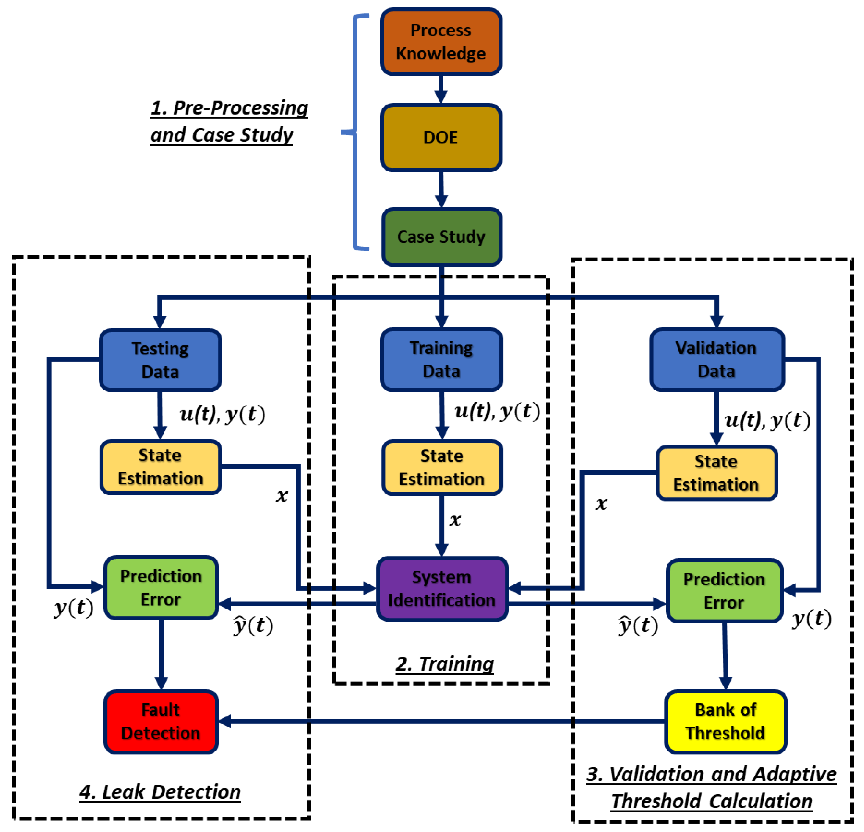
Processes 08 00474 g001
Figure 2. Novel methodology of adaptive threshold-based leak detection (ATBLD).
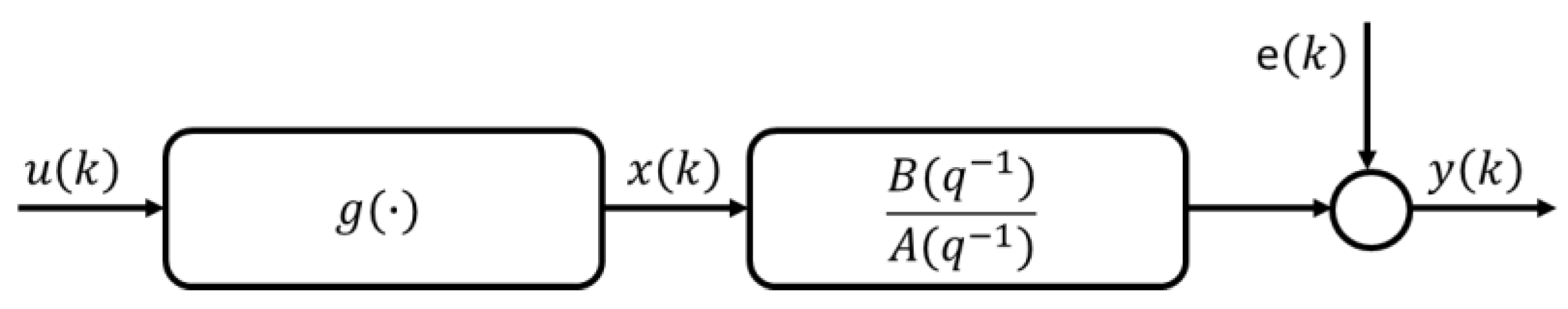
Processes 08 00474 g002
Figure 3. Block diagram representation of SISO Hammerstein model.
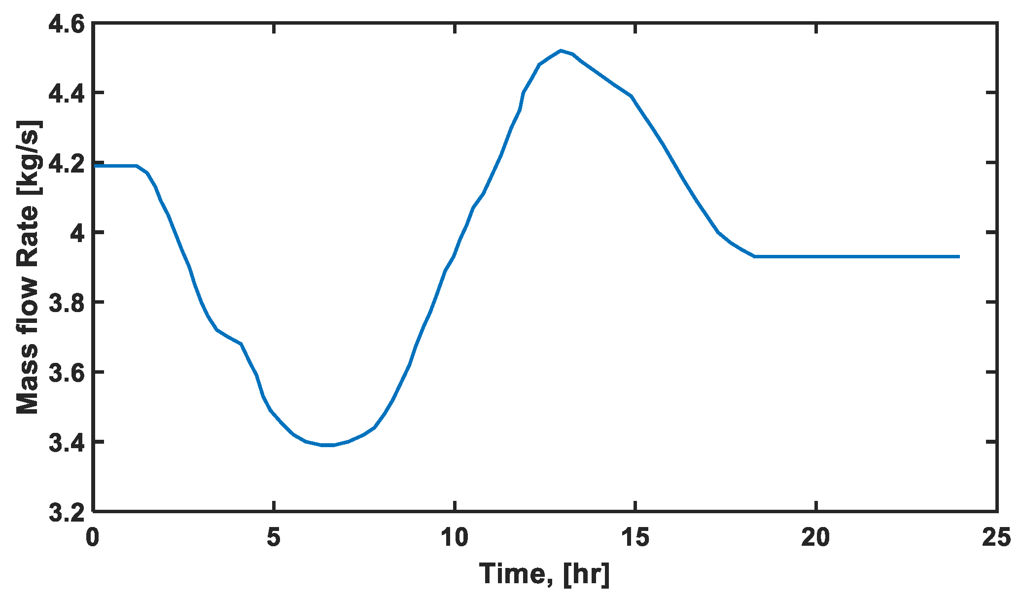
Processes 08 00474 g003
Figure 4. Mass flow rate changes at the outlet of the pipeline for validation test.
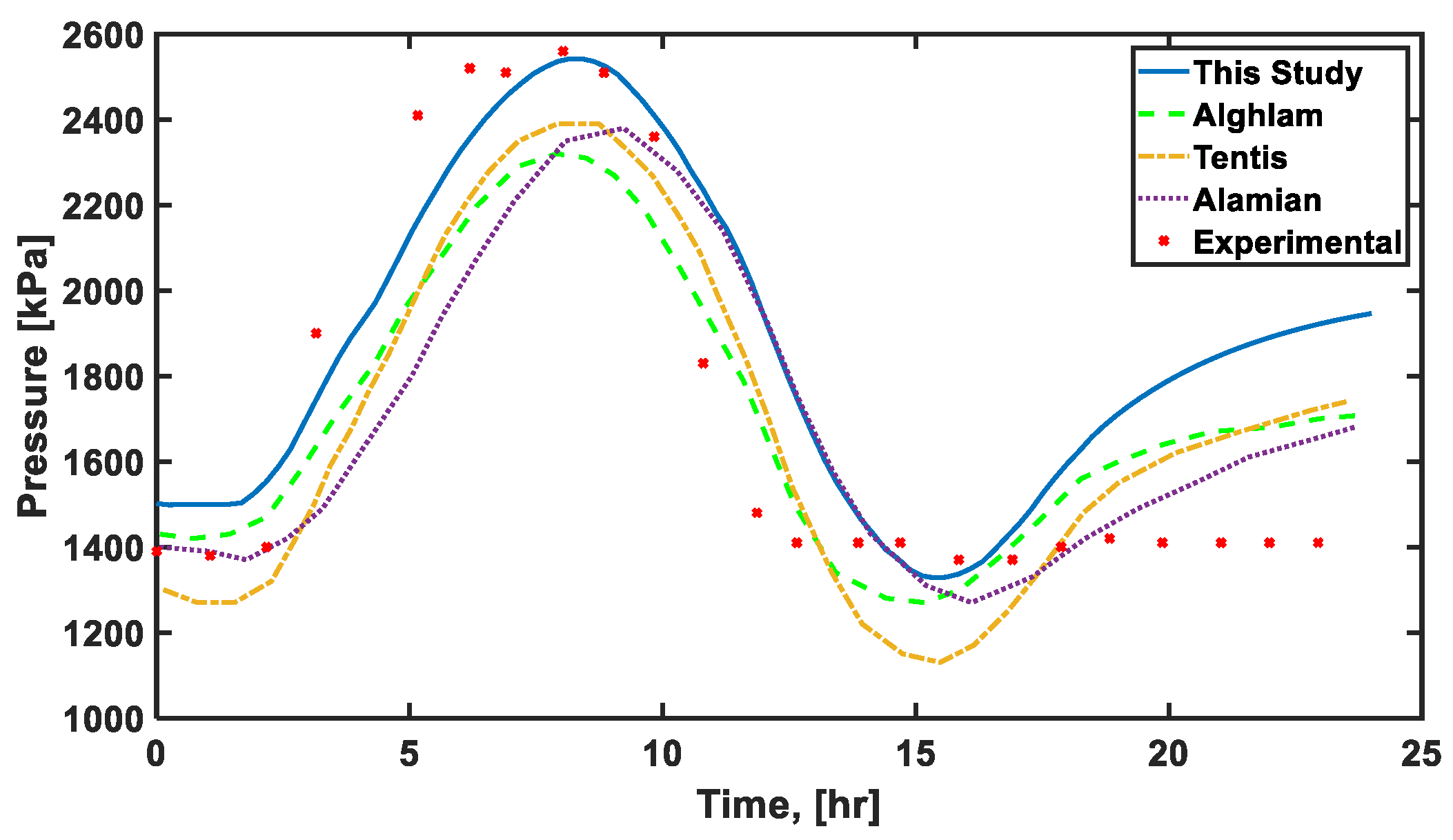
Processes 08 00474 g004
Figure 5. Pipeline outlet pressure comparison with the experimental data and other studies.
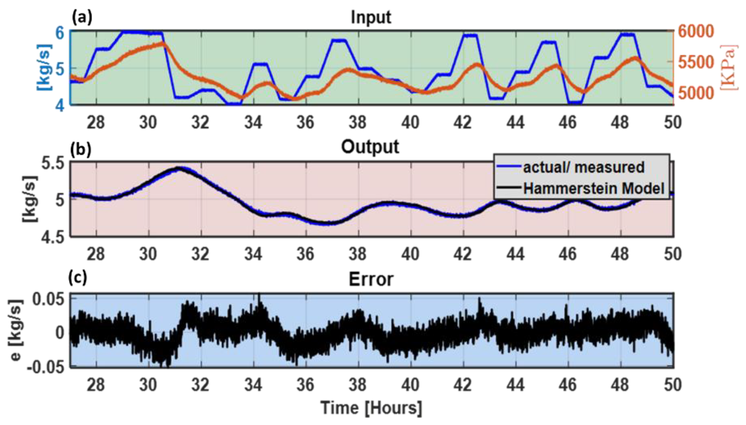
Processes 08 00474 g005
Figure 6. Hammerstein model identification results (training), (a) pressure and mass flow rate signals at inlet, used as a model input, (b) actual mass flow rate signals at outlet, used as a model output. Estimated mass flow rate sign for given input and output signals, (c) modeling errors between actual and estimated mass flow rate.
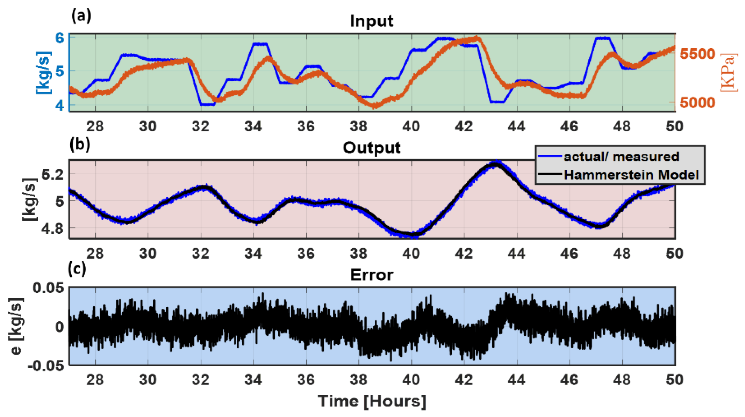
Processes 08 00474 g006
Figure 7. Validation of Hammerstein model with 1201 parameters and noise ratio of 0.2%, (a) Pressure and mass flow rate signals at inlet, used as a model input, (b) actual mass flow rate signals at outlet, used as a model output. Estimated mass flow rate sign for given input and output signals, (c) Modeling errors between actual and estimated mass flow rate.
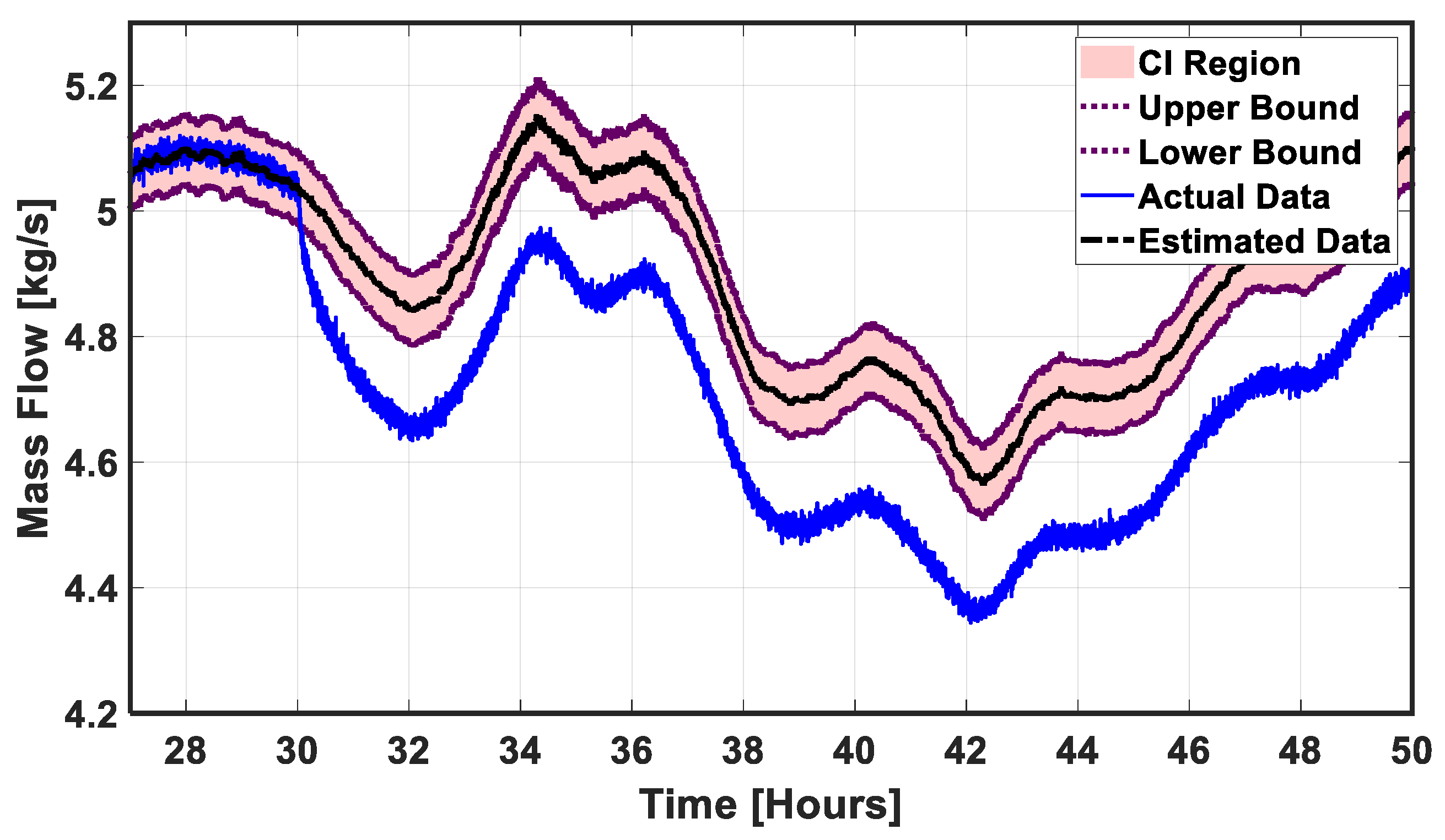
Processes 08 00474 g007
Figure 8. Testing of Hammerstein model with 0% leak at 30 h, 1201 parameters and 0.2% noise ratio.
Processes 08 00474 g008
Figure 9. Testing of Hammerstein model with 5% leak at 30 h, 1201 parameters and 0.2% noise ratio.
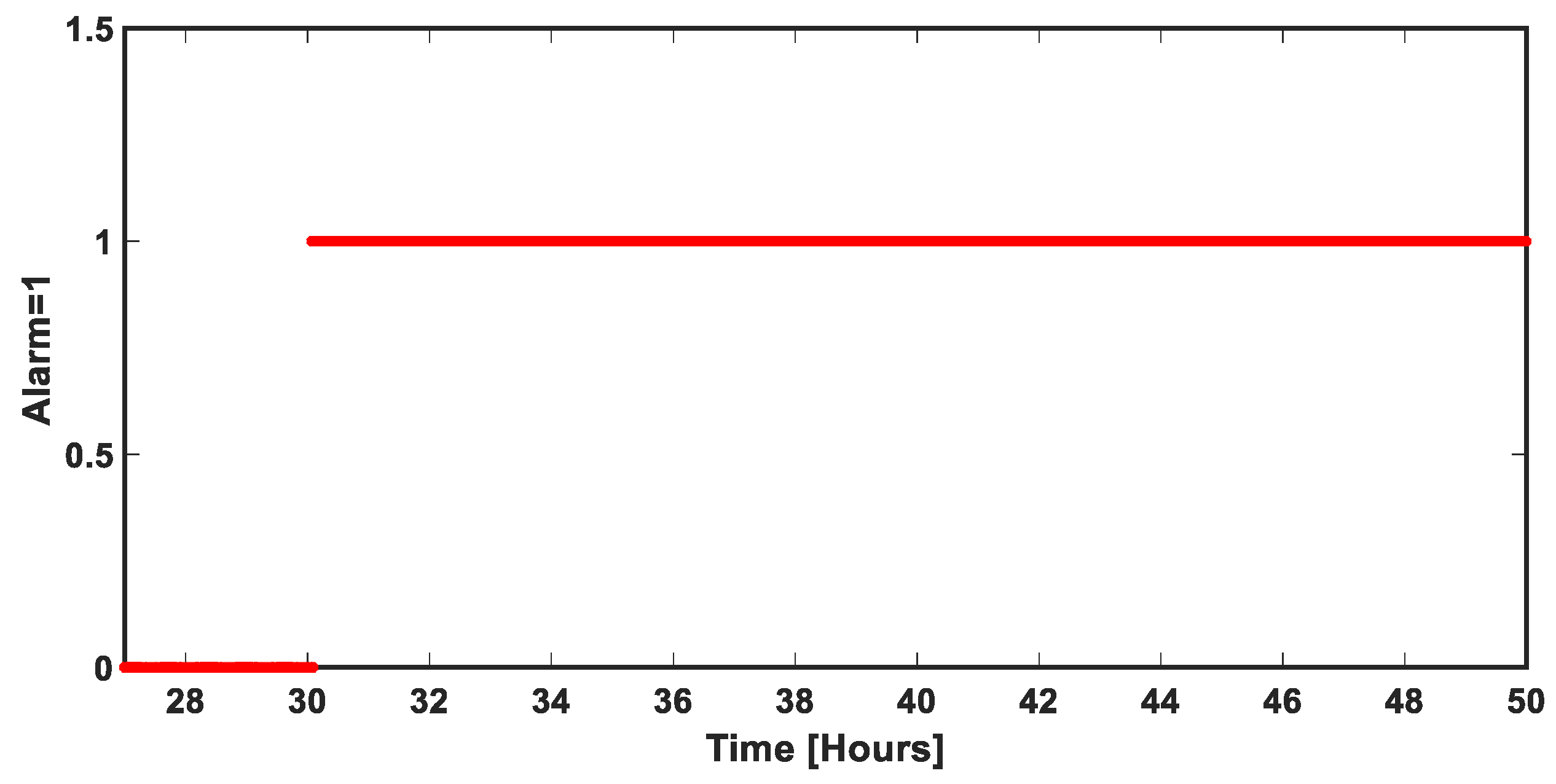
Processes 08 00474 g009
Figure 10. Binary signals indicating normal and leakage conditions.
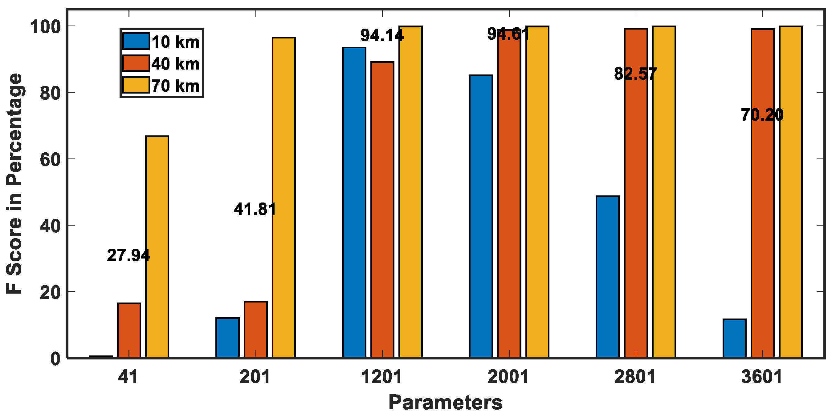
Processes 08 00474 g010
Figure 11. F-Score of 5% leak detection using various parameters at different locations.
Processes 08 00474 g011
Table 1. Variations in the parameters used by previous studies on pipeline leak detection.
FluidLength (km)1 Fluid
Compr.
2 Temp.
Variation
Detection MethodNoise (%)Leak in Terms ofFault DetectionReferences
Range/ValueAccuracy (%)
Liquid10ConstantConstantSVMNoVelocity(1–20)%99[19]
Gas Mix10TransientTransientObserver0.5Mass Flow0.7–1.5-[14]
Gas Mix0.014ConstantConstantRTTMYesOpening30 to 60 degree94[31]
Multiphase20TransientTransientANNYesOpening0.5 inch95[24]
Liquid0.0578ConstantConstantPCAYesMass Flow(4–5)%-[27]
Gas Mix35ConstantConstantObserverNoMass Flow4.1%-[34]
Liquid37TransientConstantParticle FilterYesMass Flow10%-[37]
Gas Mix0.6TransientConstantRTTMNoMass Flow30%-[32]
Liquid0.011ConstantConstantIRFYesOpening(1–2) mm-[38]
Liquid40ConstantConstantDistanceYesMass Flow1%-[16]
Gas Mix80TransientTransientHM0.0–0.5%Mass Flow(2–5)%>95This study
1 Fluid Compressibility, 2 Temperature Variation. Where, SVM = Support vector machines. RTTM = Real time transient modeling. ANN = Artificial neural network. PCA = Principle component analysis. IRF = Impulse response function HM = Hammerstein model.
Table 2. Indicators used to evaluate the performance of leak detection system.
Performance MeasureFormula
Accuracy (percentage of correct classification) T P + T N P + N × 100
Error rate (percentage of incorrect classification) F P + F N P + N × 100
Sensitivity to fault T P P × 100
Specificity (true normal condition detection) T N N × 100
False alarm rate 1 T N N × 100
Precision (true fault detection) T P T P + F P × 100
F-score 2 × p r e c i s i o n × r e c a l l p r e c i s i o n + r e c a l l × 100
Where, P = Total number of faulty samples/data points .   N = Total number of fault-free/normal samples/data points. T P = Number of correctly detected faulty samples/data points. T N = Number of correctly detected normal samples/data points. F P = Number of incorrectly detected faulty samples/data points in fault free condition. F N = Number of incorrectly detected normal samples/data points in the case of leak.
Table 3. Boundary conditions and other parameters used in case study.
ParametersCase Study
Length, Diameter80 km, 0.20701 m
Thickness of Wall0.101 m (4 inches)
Pipe materialCarbon Steel
Flowing fluidNatural Gas
Surface roughness0.617 mm
Ambient temperature283.15 K
Heat transfer coefficient 2.84   W m 2 K
Inlet temperature293.15 K
Inlet pressure-
Inlet mass flowAPRBS
Outlet pressure2 MPa
Outlet temperature283 K
Outlet mass flow-
Friction factorColebrook
CompressibilityGERG-2008
Table 4. Leak detection system performance measures with several parameters at 10 km, leak size was 5% of the nominal flow and, noise ratio was 0.2%.
Number of ParametersAc (%)ER (%)Se (%)Sp (%)Pr (%)FS (%)LDT (min)
4113.2986.700.291001000.518541.67
8113.3886.620.381001000.771083.20
20118.5981.406.3810010012.0062.83
40183.4816.5181.0010010089.5012.00
80192.367.6391.2210010095.4120.67
120189.3710.6287.7710010093.4933.17
160185.9814.0283.8710010091.2336.00
200177.9922.0074.6910010085.1622.17
240164.1335.8658.7510010074.0276.33
280141.0058.9632.1910010048.7248.70
360118.3581.646.1799.5399.8811.6316.67
480170.7029.2966.4099.3599.8579.7679.76
Table 5. Leak detection system performance measures with several parameters at 45 km, leak size was 5% of the nominal flow and, noise ratio was 0.2%.
Number of
Parameters
Ac (%)ER (%)Se (%)Sp (%)Pr (%)FS (%)LDT (min)
4120.8679.138.9910010016.51121.50
8120.7379.268.8410010016.25113.67
20121.1078.899.2710010016.97103.33
40135.3864.6125.6910010040.8726.00
80158.2441.7551.9710010068.4014.67
120182.9017.0080.3310010089.0911.00
160194.285.7193.4310010096.609.50
200197.982.0197.6810010098.828.33
240198.651.3498.4510010099.227.33
280198.501.49798.3010010099.136.33
360198.451.54798.2699.7299.9599.1012.00
480198.561.4398.4499.3599.9099.163.83
Table 6. Leak detection system performance measures with several parameters at 70 km, leak size was 5% of the nominal flow and, noise ratio was 0.2%.
Number of
Parameters
Ac (%)ER (%)Se (%)Sp (%)Pr (%)FS (%)LDT (min)
4156.6543.3450.1510010066.8091.50
8162.3437.6556.7010010072.3680.00
20194.085.9193.1910010096.4710.33
60199.420.5899.3310010099.665.50
80199.680.31499.6310010099.814.00
120199.720.2799.6810010099.843.00
160199.780.2199.7510010099.872.83
200199.730.2699.6910010099.842.67
240199.790.2099.7610010099.882.50
280199.750.24199.7210010099.863.00
360199.780.21799.7510010099.873.00
480199.570.4299.7598.4299.7699.752.50
Table 7. Leak detection system performance measures with increasing noise. Leak size was 5% of the nominal flow; 1201 parameters are used for the mass flow rate estimation.
Noise (%)Ac (%)ER (%)Se (%)Sp (%)Pr (%)FS (%)LDT (min)
0.099.730.2699.6910010099.840.17
0.199.770.2299.7310010099.863.00
0.299.750.2499.7210010099.863.00
0.399.640.3599.5910010099.793.17
0.499.560.4399.5010010099.794.00
0.599.270.7299.1610010099.583.67
Average99.620.3799.56510010099.786672.835
Table 8. Leak detection system performance measures with ascending leak sizes, noise was kept 0.2%; 1201 parameters are used for the mass flow rate estimation.
Leak Size (%)Ac (%)ER (%)Se (%)Sp (%)Pr (%)FS (%)LDT (min)
132.9967.0022.9410010037.3273.33
295.954.0695.3210010097.608.83
399.480.5199.4010010099.704.67
499.700.3399.6110010099.804.17
599.750.2499.7210010099.863.00
Table 9. Comparison between our work and recent leak detection studies.
YearDetection TechniqueAdvantageDisadvantageBest Performance UnderReference
2020Model Identification and ATBLD
-
High accuracy under transient conditions
-
Less amount of data required for training
-
Low Cost
-
Easily extended for leak localization and size estimation
-
Easy to make physical interpretations
-
Requires detailed study on design of experiment and selection of parameters
-
Detailed tuning is required for new system
Transient conditionsThis Study
2019SVM
-
Good classifier for high dimensional faults
-
Low Cost
-
Detailed tuning is required for new system
-
Difficult to make physical interpretations
-
FAR in Transients
Steady state conditions[19]
2018PCA
-
Low Cost
-
Good for Multivariate systems
-
Detailed tuning is required for new system
-
Requires addition effort to combine with other techniques, e.g., Q-Statistics
-
FAR in Transients
Steady state conditions[27]
2018IRF
-
Less amount of data are required for training
-
Low Cost
-
Easily extended for leak localization and size estimation
-
Requires detailed study on design of experiment and selection of parameters
-
Detailed tuning is required for new system
Transient conditions[38]
2017ANN
-
Low Cost
-
Once trained, then have high speed
-
Large data sets are required for training
-
Detailed tuning is required for new system
-
Very difficult to make physical interpretations
-
FAR in Transients
Steady state conditions[24]
2017Observer
-
High accuracy
-
Generic: Easily applied to any pipeline
-
Easily extended for leak localization and size estimation
-
Advanced computational facility is required
-
Required complex modeling for good results
Transient conditions[14]
2015RTTM
-
High accuracy
-
Generic: Easily applied to any pipeline
-
Easily extended for leak localization and size estimation
-
Advanced computational facility is required
-
Required complex modeling for good results
Transient conditions[31]
Where, ATBLD = Adaptive thresholds-based leak detection. SVM = Support vector machines. PCA = Principle component analysis. IRF = Impulse response function. ANN = Artificial neural network. RTTM = Real time transient modeling.

