An Improved Mathematical Model for Accurate Prediction of the Heavy Oil Production Rate during the SAGD Process

Abstract

Steam-assisted gravity drainage (SAGD) is one of the most successful thermal enhanced oil recovery (EOR) methods for cold viscose oils. Several analytical and semi-analytical models have been theorized, yet the process needs more studies to be conducted to improve quick production rate predictions. Following the exponential geometry theory developed for finding the oil production rate, an upgraded predictive model is presented in this study. Unlike the exponential model, the current model divides the steam-oil interface into several segments, and then the heat and mass balances are applied to each of the segments. By manipulating the basic equations, the required formulas for estimating the oil drainage rate, location of interface, heat penetration depth of steam ahead of the interface, and the steam required for the operation are obtained theoretically. The output of the proposed theory, afterwards, is validated with experimental data, and then finalized with data from the real SAGD process in phase B of the underground test facility (UTF) project. According to the results, the model with a suitable heat penetration depth correlation can produce fairly accurate outputs, so the idea of using this model in field operations is convincing.

1. Introduction

It goes without saying that available oil contents are recognized as an unsustainable source of fuel energy in the world, and it will not take a long time for whatever remains in conventional oil reservoirs to run out. As a result, the global demand will be more inclined toward exploiting heavy oil reservoirs, a confident energy source after the conventional one. In contrast to several other reservoir types, such as light shale reserves, where enhanced oil recovery (EOR) applications can be implemented after the primary production stage, Steam-assisted gravity drainage (SAGD) operators tend to start the process after the wells are completed. As has been vastly delineated in the literature, because it has viscosities that are too high, the oil in heavy oil reservoirs cannot move naturally. Thus, researchers have been developing various methods to give companies the ability to practically deal with the problem [1,2]. Among the different methods, it appears that thermal methods are more convincing than others. One of the thermal methods, which has a huge reputation in extracting heavy oil, is the SAGD process (or its variations). Figure 1 shows a simplified demonstration of this process. As can be seen, the reservoir is drilled with at least a pair of horizontal wells for the SAGD process to progress [3]. Steam is injected from the upper horizontal well (named injector) and the heated oil is summoned up from the well located at the bottom of the reservoir (named producer). The role that steam plays is to transport heat to the viscous, cold areas in the pay zone. There, the conduction mechanism has its foremost effect in heating the untouched oil. While the untouched heavy oil gradually becomes warmer, its viscosity sharply decreases and consequently, thanks to the gravity force, flows down toward the producer [4].

In general, the simulation of a reservoir in a SAGD process is performed by two methods. The first one originates from numerical methods, which include many equations and sheer conditions [6]. Almost all commercial software related to petroleum engineering uses this method. It is believed that numerical methods express accurate results in different EOR manners [6,7,8], since they take into account all governing equations, including all transform phenomena expressions and thermodynamic equations of state. However, its most noteworthy flaw that ought to be highlighted is the weaknesses in quickly converging on the ultimate results [7], which has made researchers seek other methods. That is why petroleum engineers have been developing an alternative to overcome this issue. SAGD analytical models, as a second method, tend to adapt the main in-situ mechanisms and processes that occur during the oil production stage. Researchers have usually made many simplifying assumptions to obtain an equation capable of rapidly predicting the oil production rate in SAGD. In addition to accurate outputs, attempts were made for the developed equation(s) to require fewer reservoir input data to yield the desired outputs [9].

The first person to model the SAGD process was Butler [10]. In 1981, according to different observations from some SAGD tests, Butler and Mac Nab [10] developed the first simple mathematical formula to predict the production rate of the heated oil in their experimental model. Similarly to what is depicted in Figure 1, they assumed that a steam chamber is formed as superheated steam is injected into the reservoir through the injector. Moreover, they defined a thin layer of oil between the steam chamber and the cold oil region as the interface. As the heated oil flows down toward the producer, the interface grows sideways to reach the walls of the bed. Therefore, Butler and Mac Nab [10], using Darcy’s law, heat conduction, and also a mass balance in the vicinity of the interface, formulated the sideways expansion of the steam chamber at steady state conditions. It should be mentioned that their outcomes were not very precise in comparison to the experimental data. Again, it was Butler [11] who came up with a new idea in 1985. To modify his previous work, he changed the steady state conditions that were assumed in the earlier work. As he stated, the major problem in all preceding equations was assuming a steady temperature distribution along the interface. It was quite non-realistic and yielded inaccurate results. Thus, to overcome this shortcoming, he divided the interface into several segments and then, applied the mass and energy balances to each. In his new model, each segment (element) independently moves sideways with its own specific velocity, and the location of interface as well as the oil drainage rate was forecasted more accurately.

Several years later, a linear geometry model was suggested by Reis [12] to find out more confident results under steady state production rates. Having introduced steam-oil interface as a straight line moving at a velocity U, Reis combined all governing equations in an element of interface to form a single oil production equation as follows:

$$q_o=\sqrt{\frac{\phi \Delta S_o{k}_{o}gH\alpha }{2a{\upsilon }_{os}m}}$$

(1)

which shows the oil drainage rate from one side of the steam-oil interface. Equation (1) has the following parameters:

$q_o$ = oil production rate

$\phi$ = porosity

$\Delta S_o$ = initial oil minus residual oil saturation of system

$k_o$ = oil permeability

$H$ = reservoir height

$\alpha$ = thermal diffusivity of reservoir

$a$ = coefficient of velocity

${\upsilon }_{os}$ = oil viscosity at steam temperature

$m$ = coefficient of viscosity

Nonetheless, Equation (1) shows the independency of the oil production rate from time, which compared with other models, does not look desirable.

Later, it was Pooladi-Darvish [13] who used Butler’s idea and the HIM (heat integral method) theorem in order to change the energy balance PDE (partial differential equation) over an interface segment into a simple ODE (ordinary differential equation). In this way, Pooladi-Darvish et al. [13] stated the SAGD process as a moving boundary layer problem and imagined an exponential or polynomial equation for the temperature distribution profile ahead of the interface layer. Eventually, he modified the performance of Butler’s model [11] in a tremendous way. Similarly to what Pooladi-Darvish et al. [13] had done in his work, Rabiei et al. [14] developed a semi-analytical model to estimate the amount of oil drainage in a steam-solvent gravity process. In fact, they involved the solvent and thermal layer in the interface layer in the expanding solvent steam assisted gravity drainage (ES-SAGD) process. HIM was used to find the distribution of the solvent concentration and temperature ahead of the steam/solvent-oil interface. Next, the inverted triangle theory first introduced by Reis [12] was employed to obtain the oil flow rate. Then, they compared their model with a numerical simulator to prove the accuracy of their model. Finally, it was postulated that the ES-SAGD process had a better potential in oil recovery than the general form of the SAGD process.

Regarding Reis’s linear geometry model, Azad and Chalaturnyk [14] suggested a circular steam chamber shape for the sideways expansion of the chamber. Like Reis, they defined the flow potential function ∇Φ such that the increase in the chamber’s diameter in each time step influences Darcy’s equation results and the production rate. Aside from that, they considered the oil reservoir as circular slices and could replace the constant relative permeability with varying relative permeability in Darcy’s equation. They assumed three different possible steam chamber locations for their circular model. Consequently, as the first researchers, they could develop a semi-analytical model to simulate the beginning of a SAGD process when the steam chamber was forming. Despite a huge success in production prediction, this model is unable to show the real chamber shape when a SAGD process is in operation. The idea of presenting a model to delineate a conical steam chamber shape is more convincing. This was why Sabeti et al. [15] proposed an exponential geometry for the interface locations to compensate the obvious problem in Reis’s [11] and Azad’s [14] models. More explanation about the exponential geometry approach will be presented in the next section. But concisely, instead of the linear assumption based on Reis’s theory, the interface location was plotted by such the exponential function of $f(x)=C(1-{\mathrm{e}}^{-bx})$. Finally, Equation (2) was derived as oil production rate related to the SAGD process:

$$q_o=\sqrt{\frac{\phi \Delta S_o{k}_{o}gH\alpha }{2a{\upsilon }_{os}m}}.\sqrt{2\left[\left(H-C\right)-\frac{H}{\ln \left(1-\frac{H}{C}\right)}\right]\sqrt{1+{\left(\frac{1}{bC}\right)}^2{e}^{-2\ln \left(1-\frac{H}{C}\right)\frac{1}{L}}}}$$

(2)

where, b and C are dimensionless coefficients and L represents the length of the steam-oil interface layer. Compared with Equation (1), Equation (2) has a second term which implicitly defines the influence of the interface curvature over the amount of the production rate. Compared with the old version of the SAGD models, this exponential geometry had a promising accuracy in both the interface location and the oil production rate. Shi and Okuno [16] took Reis’s idea and temperature variation along the edge of a steam chamber account to develop an analytical model to estimate oil production rate and steam oil ratio (SOR) in the Surmont SAGD project.

Taking into account all aforementioned studies and following our previous work, the authors of this study decided to move one step further to increase the similarity between the mathematical model and the real mechanism behind the SAGD process. To adapt the exponential geometry model to the real conditions, the assumption of $\nabla \mathsf{\Phi }=g\frac{H}{L}$ must be obviated from the model. To do so, this paper recommends that the exponential interface, as an analogy for the steam-oil interface, be divided into several segments so that the more appropriate relation, $\nabla \mathsf{\Phi }=g\sin \theta$, can be used in the mathematical formula. The present work also uses temperature variation ahead of each segment of the steam-oil interface to find the flowing oil rate.

2. Theory

At the SAGD process, steam is injected from the top well in a reservoir, and the drained oil goes out from the bottom well. Meanwhile, three different scenarios happen respectively. The operation starts by developing a steam chamber, and it may need a thermal circulation process for a while before the producer well can play its own role in the SAGD process. After the steam chamber touches the cap rock, the second stage starts. In this stage, the oil production occurs along with the sideways expansion of the steam chamber. Afterwards, when the steam chamber has completely expanded to the reservoir boundaries, the falling phase begins. In the third stage, the height of oil reservoir begins to gradually descend and at the same time, the oil production rate drops, too. The study described in this work encompasses the second and third stages of a real SAGD process, therefore, it is clear that the equations deployed here are not applicable in the first stage at all. It is worth mentioning that the first stage matters to some researchers, such as Zargar [17] and Irani [18], and they presented their own equations.

The flow of the heated oil ahead of the interface layer complies with the Darcy’s law in the porous media. As shown in Figure 2, for a tiny element ahead of the steam-oil interface, the production rate is formulated as:

$$d{q}_o=\frac{k{\rho }_o}{\mu }\nabla \mathsf{\Phi }d\xi$$

(3)

in which, the following parameters are included:

$dq$ = differential oil flow

$d\xi$ = distance from interface

$\nabla \mathsf{\Phi }$ = the flow potential function

As mentioned before, unlike the exponential geometry model [5], the flow potential function is calculated in this way:

$$\nabla \mathsf{\Phi }=g\sin \theta$$

(4)

where, θ represents the angle between the steam-oil interface and horizontal line.

To find the oil viscosity ahead of the interface layer, the equation suggested by Butler [11] is used:

$$\upsilon \left(\zeta \right)=\frac{{\upsilon }_{os}}{\exp \left(-\frac{m\zeta }{\gamma }\right)}$$

(5)

In Equation (5), Butler simply related the oil viscosity at distance $\zeta$ to heat penetration depth, $\gamma$. Now, combining Equations (3)–(5), the oil production rate is calculated:

$$q_o={\displaystyle \underset{0}{\overset{\infty }{\int }}\frac{kg\sin \theta }{\frac{{\upsilon }_{os}}{\exp \left(-\frac{am\zeta }{\gamma }\right)}}}d\zeta =\frac{k\gamma g\sin \theta }{m{\upsilon }_{os}}$$

(6)

In this survey, the steam chamber is depicted as the exponential function of Equation (7) in which C and b are coefficients that determine the curvature of the steam chamber interface during the steam injection:

$$f\left(x\right)=C\left[1-e^{-bx}\right]$$

(7)

It was shown that the above exponential function has the ability to locate the interface pertinently with respect to the linear geometry demonstrated by Reis [11], hence, the authors of this study take advantage of Equation (7) again. Using Equation (7), the amount of $\sin \theta$ can be defined as:

$$\sin \theta =\sqrt{\frac{1}{1+\frac{1}{{\left(Cb\right)}^2}{e}^{2bx}}}$$

(8)

If Equation (8) is plugged into Equation (6), the final oil production rate with respect to time is obtained:

$$q_o=\frac{k\gamma g}{m{\upsilon }_{os}}\sqrt{\frac{1}{1+\frac{1}{{\left(Cb\right)}^2}{e}^{2bx}}}$$

(9)

The only parameter that so far remains unknown is the heat penetration depth. Many studies have been conducted to find $\gamma$ [11,13,14,20,21,22]. As an example, here is an equation derived by Butler [11], which is used in developing the new flow rate equation presented in this study:

$$\frac{d\gamma }{dt}=\frac{2}{\pi }\left(\frac{\alpha }{\gamma }-U_v\right)$$

(10)

To get Equation (10), an energy balance on the element defined in Figure 2 is required (see Appendix A). This differential heat equation asserts that the gradient of penetration depth with respect to time is inversely proportional to its own amount, and that linearly varies with the velocity $U_v$ perpendicular to the interface. According to Equation (10), it makes sense that the model needs the velocity of each segment to calculate the penetration depth in each time step. By performing a lumped mass balance over the whole area of the reservoir, as is shown in Figure 3, the maximum frontal velocity $U_m$ is computed. In this case, the total oil production is equal to the swept area in the reservoir, which covers the same area as the steam chamber inside the reservoir does. Thus,

$$Q_o=\phi \Delta S_o\left(H{W}_S-{\displaystyle \underset{0}{\overset{W_s}{\int }}C\left(1-e^{-bx}\right)dx}\right)$$

(11)

where H and W_s represent the reservoir height and the half-width of the steam chamber, respectively. Equation (11) is differentiated with respect to time as shown in the following line:

$$q_o=\frac{d}{dt}\left[\phi \Delta S_o\left(H{W}_S-{\displaystyle \underset{0}{\overset{W_s}{\int }}C\left(1-e^{-bx}\right)dx}\right)\right]$$

(12)

Now, by manipulating Equation (12), the required relation for locating the steam-oil interface as well as the penetration depth is obtained:

$$U_m=\frac{q_o}{\left[\phi \Delta S_o\left[\left(H-C\right)-\frac{H}{\ln \left(1-\frac{H}{C}\right)}\right]\right]}$$

(13)

The maximum velocity, which is believed to occur at the top of the interface, has the following relationship with the velocity perpendicular to it:

$$U_m=\frac{U_v}{\sin \theta }$$

(14)

Having the maximum velocity ($U_m$) available from Equation (14), the location of the top of the interface can be found at each time step:

$$W_{s,n+1}=U_m\times \Delta t+W_{s,n}$$

(15)

where $\Delta t$ indicates a time interval and n denotes the number of the time intervals which increases with the passing of time. Following the new width of the steam chamber, an interface velocity for each segment can be calculated with the following chain of formulas:

$$H=C\left(1-e^{-b{W}_s}\right)\to b_{n+1}=\frac{-\ln \left(1-\frac{H}{C}\right)}{W_{s,n+1}}$$

(16)

$$\Delta x_i=\left(\frac{-\ln \left(1-\frac{Z_i}{C}\right)}{b_{n+1}}\right)-\left(\frac{-\ln \left(1-\frac{Z_i}{C}\right)}{b_n}\right)$$

(17)

Here, subscript i indicates each segment number of the interface:

$$\Delta U_{m,i}=\Delta x_i/\Delta t$$

(18)

In the previous paper (the exponential geometry model), the heat penetration depth through the interface does not appear in the oil drainage rate equation. But in this work, it clearly does (pay attention to Equation (9)). Please note that, the more accurately the heat penetration depth is used in Equation (9), the more accurately results are obtained through solving the equation.

The procedure for finding the amount of steam required for a SAGD process is the same as that introduced by Sabeti et al. [5]. The three main sources of energy consumption in SAGD consist of that to keep the steam chamber warm, that to keep the interface heated, and that lost to the overburden. Eventually, after some manipulating, the equation which represents the required steam rate to proceed with the SAGD process is obtained by:

$${Q^{\prime }}_{inj}=M_R\Delta T\left[U_m\left(\left(H-C\right)-\frac{H}{\ln \left(1-\frac{H}{C}\right)}\right)+\frac{\alpha }{a}\frac{d\left(\frac{L}{U_m\sin \theta }\right)}{dt}+2\sqrt{\frac{\alpha }{\pi }}{U}_m\sqrt{t}\right]$$

(19)

where ${Q^{\prime }}_{inj}$ and $M_R$ are the rate of latent heat injection and formation heat capacity of the reservoir, respectively. To get the interface length by using Equation (7), the following function can be defined:

$$L=\frac{1}{2b}{\left[\begin{array}{l}2\ln \left(1+\sqrt{1+C^2{b}^2{e}^{-2bx}}\right)-2\left(1+\sqrt{1+C^2{b}^2{e}^{-2bx}}\right)\\ -\ln \left(C^2{b}^2{e}^{-2bx}\right)\end{array}\right]}_0^x$$

(20)

3. Computation Procedure

In order to find the production rate, interface location, interface velocity, temperature distribution ahead of interface, and the amount of steam required to complete a SAGD process, the following sequence needs to be implemented. Nonetheless, before that, the height of the reservoir should be divided into some evenly distributed segments, as displayed in Figure 4.

(1)

Using Equation (2), the amount of oil production rate is calculated as a first supposition.

(2)

The value of the maximum horizontal velocity is found by Equation (13).

(3)

Equations (15)–(17) are used to find the location of the interface. Furthermore, the magnitude of horizontal velocity at each segment is obtained by Equation (18).

(4)

Having U_v and $\gamma$ and applying Equation (10), the value of the heat penetration depth $\gamma$ for the next time step is calculated. The first value of the heat penetration depth $\gamma$ at time t = 0 for each segment of the steam-oil interface needs to be estimated.

(5)

To get the value of the oil production rate, Equation (9), with its required parameters (formerly defined in the previous steps), is used.

(6)

The calculated $\gamma$ should not have a significant discrepancy with its previous value. To fulfill this, the new $\gamma$ should be recalculated with the new values from step 2.

(7)

In the end, regarding an accurate oil production rate, Equations (19) and (20) are employed to get the energy required for the SAGD process.

Repeat steps 2 through 7 until the final time step is reached.

4. Results and Discussion

This section is aimed at validating the new semi-analytical model, and then applying it to a field reservoir under real-world conditions. To do so, one of well-known experimental works recorded by Chung and Butler [23] was used.

Table 1. Property list of the SAGD experiment [23]. Reproduced with permission from (Chung and Butler), (Annual Technical Meeting); published by (Society of Petroleum Engineers), (1986).

Properties	Value
Permeability	9.44 × 10−10 ${\mathrm{m}}^2$
Thermal diffusivity	5.87 × 10−7 ${\mathrm{m}}^2/\mathrm{s}$
Porosity × Saturation ($\phi \times \Delta S$)	0.37
m	3.6
Height of the bed	0.21 $\mathrm{m}$
Formation Width	0.175 $\mathrm{m}$
Steam Temperature	109 $℃$
Oil viscosity at steam temperature	104 × 10−6 ${\mathrm{m}}^2/\mathrm{s}$
Coefficient of velocity $\left(\mathrm{a}\right)$	0.4
Thickness of the bed	0.03 $\mathrm{m}$
Oil density	980 $\mathrm{kg}/{\mathrm{m}}^3$

represents the physical properties of the oil and reservoir that they considered in their tests. They used Ottawa sand as porous media and saturated it with Cold Lake bitumen at room temperature. The experiment was conducted in two discrete well configurations, A and B. Here, well configuration B, which is in compliance with the present model, was chosen for more investigation. The distance between the producer and injector was set to 20 cm in well configuration B. In SAGD, unlike other EOR processes, the injected fluid does not push the oil back. Thus, before an experiment was started, they applied a steam circulation through the injector for 30 min to form an initial communication path between the two wells.

It must be mentioned that test B does not have the first step (rising of the chamber) in the SAGD process. Therefore, its recorded results are certainly closer to the presented mathematical model in comparison to test A. In Figure 5, the results of this new model are compared with the recorded data (test B) from Chung and Butler [23], as well as outputs from the exponential model. It was assumed that the scale coefficient C in Equation (9) and the heat penetration depth $\gamma$ had the values of 2.25 × H and 0.15 × H, respectively. 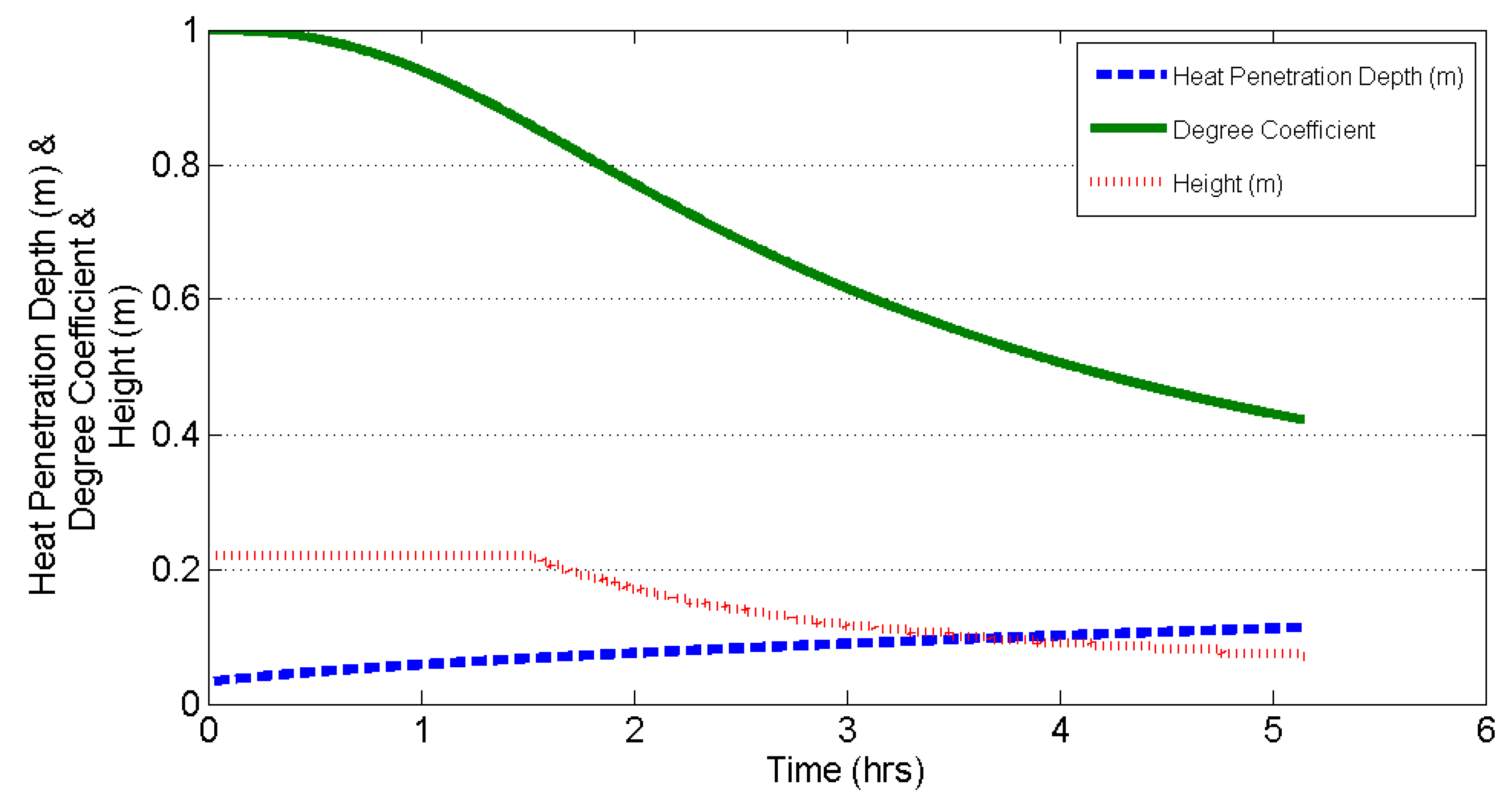The oil production rate, seen in Figure 5, is approximately constant in both the experimental data and the exponential model from the beginning of the experiment for about 1.5 h, due to the expansion of the steam chamber toward the formation boundaries. After that, the oil production rate follows a falling trend as the reservoir becomes depleted. The oil production rate follows a very similar trend, according to the results of the new model and the experiment. However, at the beginning of the process, the mathematical model predicts a lower production rate, which can be understandably attributed to the first estimation of the heat penetration depth in step 3 of the proposed solution algorithm. Equation (9) includes the three important parameters of heat penetration depth, the angle of interface with respect to horizontal, and the formation height, each of which automatically affects the production rate. Using Equation (10) in the solving procedure, the amount of heat penetration in each segment can be expected to gradually increase. The steady rise of the last segment’s depth on the interface as time goes on is shown in Figure 6. This increment influences the production rate. However, although the proposed model presents an increase in the depth, as shown in Figure 7, there is a reduction in the formation height and the interface angle simultaneously. While the penetration depth directly increases the oil production rate, the reductions in formation height as well as the interface angle indirectly lower the production rate. Eventually, these changes lead to a decreasing trend in the production rate (as shown in Figure 5 after 1.5 h). Please note that Equation (10) takes into account the two extremes (see Appendix A) and is not exact. Furthermore, using Equation (10), one may notice the unrealistic non-stop rise of the heat penetration depth with time. Thus, taking that into account, the new model cannot give very accurate results in comparison with the experimental data, as illustrated by Figure 5.

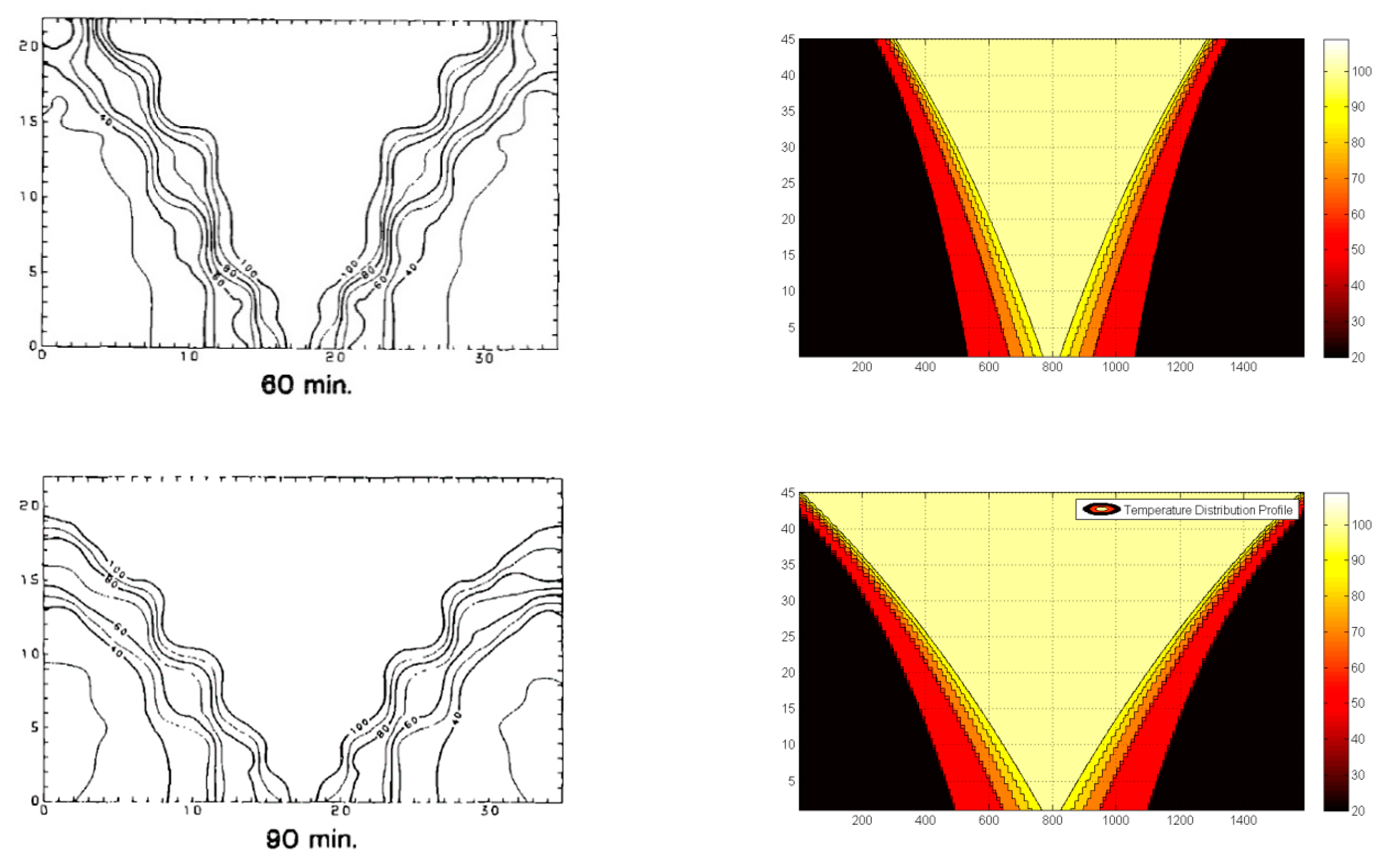
In order to show the importance of the new model, the temperature distribution in the reservoir at various times has been sketched in Figure 8. Isothermal lines are clear in both the simulation and experimental cases. The contour plots designed by the model fairly agree with Chung and Butler’s [23] thermal screenshots. It appears that after 1 h, when the production rate reaches its peak, the steam chamber is fully expanded across the reservoir and starts its falling phase. The value of C in the exponential function (Equation (7)) has the potential to change the curvature of the isothermal lines in Figure 8. In other words, the more curved the isothermal lines, the lower the value of the scale coefficient.

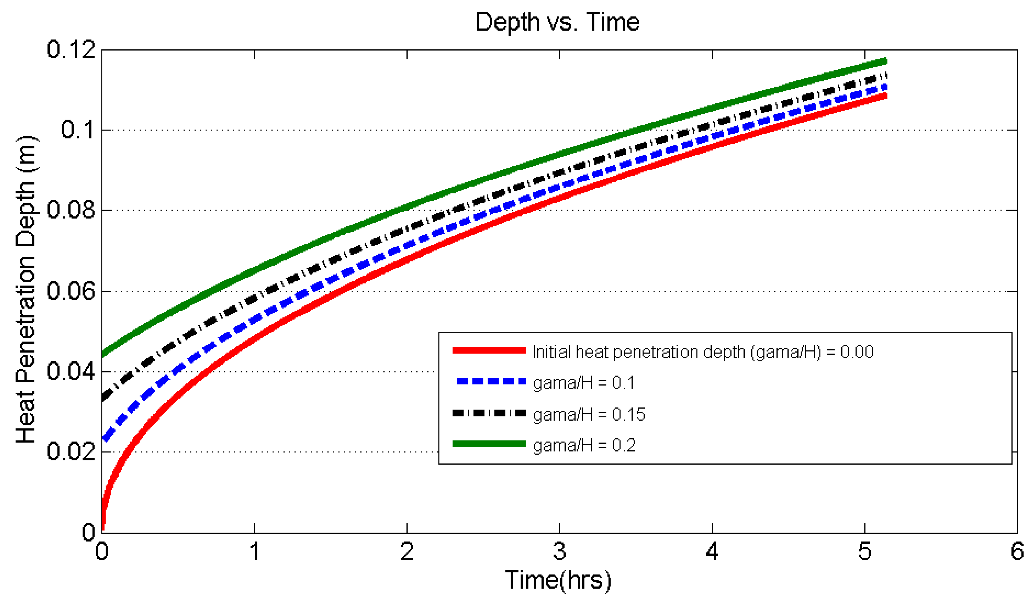
It is worthwhile to determine if the initial estimation for the value of heat penetration depth ($\gamma$) has a considerable impact on the oil production rate. Theoretically, it does not hugely affect the results. However, in order to scrutinize its influence, several runs have been taken with different initial estimates. As expected, the higher the initial estimate for the heat penetration depth, the higher the prediction of Equation (10). In the same way, as can be seen in Figure 9, as the time passes, higher initial estimates create higher values for the heat penetration depth. Apart from that, Figure 10 represents various outputs coming from these initial estimates. At the first glance, it may be concluded that there are huge discrepancies among different cases at the beginning of the process. However, they gradually demonstrate similar trends after passing their peaks and converge to a production rate of 20 gr/h. As a result, the first estimate does not actually limit the use of this method in other reservoirs with different properties.

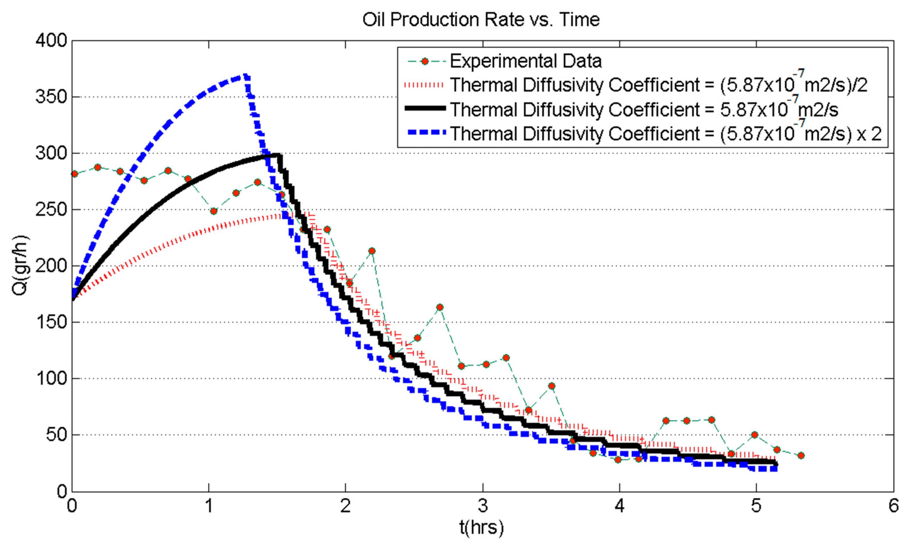
As conduction is the main heat transfer mechanism in SAGD, thermal diffusivity is a key parameter in transferring heat to oil. To study the effect of thermal diffusivity on oil production in SAGD, three different values of thermal diffusivity were selected in the model under study. The values are half of, equal to, and twice the value of those mentioned in Table 1. The resulting oil production rates in the three cases during SAGD production are shown in Figure 11. As can been seen, the higher thermal diffusivity, the higher oil the production rate, especially at the beginning of the process. Conductive heat transfer occurs at a higher rate across the reservoirs with a higher thermal diffusivity, which in turn raises the temperature ahead of the steam interface. In fact, in a reservoir with a higher thermal diffusivity, the heat transfer is enhanced and higher oil production rates occur.

5. Model Verification Using the UTF Project Phase B

Aside from validating the new model with the pilot test, one might want to know if it is accurate enough to estimate both the oil production rate and the amount of steam required in a real SAGD project. To find out, the properties of the Athabasca reservoir in phase B of the UTF project were used. A summary of reservoir properties is listed in

Table 2. Athabasca reservoir properties, the UTF project, Phase B [5]. Reproduced with permission from (Sabeti et al.), (Journal of Petroleum Science and Engineering); published by (Elsevier), (2016).

Properties	Value
Permeability	7 × 10−12 ${\mathrm{m}}^2$
Thermal diffusivity	6 × 10−7 ${\mathrm{m}}^2/\mathrm{s}$
Porosity × Saturation ($\phi \times \Delta S$)	0.21
m	4
Height of the bed	21 $\mathrm{m}$
Formation Width	500 $\mathrm{m}$
Reservoir Temperature	7 $℃$
Steam Temperature	220 $℃$
Oil viscosity at steam temperature	7.95 × 10−6 ${\mathrm{m}}^2/\mathrm{s}$
Coefficient of velocity $\left(\mathrm{a}\right)$	0.4
Oil density	882 $\mathrm{kg}/{\mathrm{m}}^3$
Steam quality	0.95
Formation heat capacity	1955 $\mathrm{kj}/{\mathrm{m}}^3·℃$

. In 1993, phase B of the UTF project was initiated by drilling three pair wells, all of which had a length of 500 m and were located 70 m apart from each other at a depth of 22 m [24,25]. The process continued until 1998, when its investors decided to modify the process by adding solvents into the injectors [24,26].

Introducing all the data in Table 2 to the solution algorithm designed in the previous sections produced diagrams for both oil production and steam injection rates, as demonstrated in Figure 12. Two important facts must be remembered about these diagrams. When the UTF project was started in 1993, the steam chamber began to form its usual conical shape as the first stage of the SAGD process. This lasted almost a year, and during this period, the oil production rate from each well kept growing before reaching a plateau. Firstly, the oil production diagram in Figure 12 does not take into account the production data before 1994. Secondly, when the new model was employed using the Athabasca data, it was observed that the value of heat penetration depth encroached its real size. Therefore, a maximum value was set as a constraint to prevent its excessive growth. To do so, the maximum thickness ${\gamma }_{\max }$ of the interface was assumed to be an unknown adjustable parameter. That value was determined by introducing an objective function, such as the time-weighted root-mean-squared relative error defined by Li et al. [27] (see Appendix B). By optimizing that objective function, the value of the maximum depth ${\gamma }_{\max }$ was calculated to be about 2 m. Despite these two stipulations, Figure 12 asserts the potential of the proposed model in predicting SAGD processes in homogenous formations. Not only does the oil production rate show good compatibility with the field data, but also, the amount of steam per day follows a logical and acceptable estimation.

6. Conclusions

In this study, an effort was made to introduce a fast, reliable, and valid model for the SAGD process in order to accurately predict the oil production and steam injection rates, as well as the location of the interface at different times. The new model was derived by holding onto most of the assumptions in the latest version of the SAGD model (exponential geometry). It was indicated that the model needed the steam-oil interface to be divided into equal segments for its semi-analytical approach to obtain an equation for the oil production rate. The outcomes of the model were then evaluated by the experimental data from Chung and Butler [23], and results showed an acceptable coincidence between them. It was further found that the rate of oil production is affected by three main parameters: heat penetration depth ahead of the interface, the angle of interface with respect to the horizontal line, and height of the formation. When the heat penetration depth gradually increases, the formation height, as well as the interface angle, declines with time. Thus, their combined effect makes a downward trend in the diagram of the heavy oil production rate versus time. Moreover, having a reliable correlation for heat penetration depth was proven to be vital. Hence, an erroneous estimate of this would negatively affect the accuracy of the oil production rate, steam injection rate, and the interface location in the SAGD process. Finally, the proposed model was run using the data from phase B of the UTF project. The outputs matched fairly well with the field data.