Process Drive Sizing Methodology and Multi-Level Modeling Linking MATLAB^® and Aspen Plus^® Environment

Abstract

Optimal steam process drive sizing is crucial for efficient and sustainable operation of energy-intense industries. Recent years have brought several methods assessing this problem, which differ in complexity and user-friendliness. In this paper, a novel complex method was developed and presented and its superiority over other approaches was documented on an industrial case study. Both the process-side and steam-side characteristics were analyzed to obtain correct model input data: Driven equipment performance and efficiency maps were considered, off-design and seasonal operation was studied, and steam network topology was included. Operational data processing and sizing calculations were performed in a linked MATLAB^®–Aspen Plus^® environment, exploiting the strong sides of both software tools. The case study aimed to replace a condensing steam turbine by a backpressure one, revealing that: 1. Simpler methods neglecting frictional pressure losses and off-design turbine operation efficiency loss undersized the drive and led to unacceptable loss of deliverable power to the process; 2. the associated process production loss amounted up to 20%; 3. existing bottlenecks in refinery steam pipelines operation were removed; however, new ones were created; and 4. the effect on the marginal steam source operation may vary seasonally. These findings accentuate the value and viability of the presented method.

1. Introduction

Cogeneration and polygeneration systems are an essential part of industrial production of materials and energies, consuming or generating heat, electricity, mechanical, and chemical energy [1,2]. Ambitious efforts of national and European institutions to reduce greenhouse gases emissions and to ensure sustainable industrial production [3,4,5,6,7,8,9] at the same time cannot be successfully met without increasing material and energy efficiency of the industry [10,11,12,13] by simultaneous energy, economic, environmental, and risk and safety optimization [14,15,16] of existing industrial cogeneration and polygeneration systems [17,18].

Efficient steam production, and its transport and use for both process heating and polygeneration purposes, has been targeted on various complexity levels in numerous recent studies [19,20,21,22,23,24,25,26,27,28,29,30,31,32,33,34,35,36,37,38]. Starting with techno-economic studies optimizing the efficiency of a single equipment unit [24,27,30,34,35], through steam consumption optimization in a single production unit [25,32,38,39], and cogeneration potential exploitation [19,33,36,40,41] to total site heat and power integration [20,21,22,23,28,33,37,42], the goal is always to reduce operational expenses, improve steam system stability, and decrease fuel consumption in industrial plants. Steam system topology and the impact of pressure and heat losses from steam pipelines on optimal cogeneration system sizing and operation has been addressed in several papers [22,37,43,44,45], but most studies consider neither off-design operation of steam turbines nor variable steam pressure levels as important aspects in the optimization procedure. A systematic method comprising characteristics of a real steam system operation [35,46] (variable pipeline loads, steam pressures, and temperatures) as well as real process steam/work demands has the potential to fill the knowledge and experience the gap between the modeling approach in utility systems’ optimization and real steam system operation.

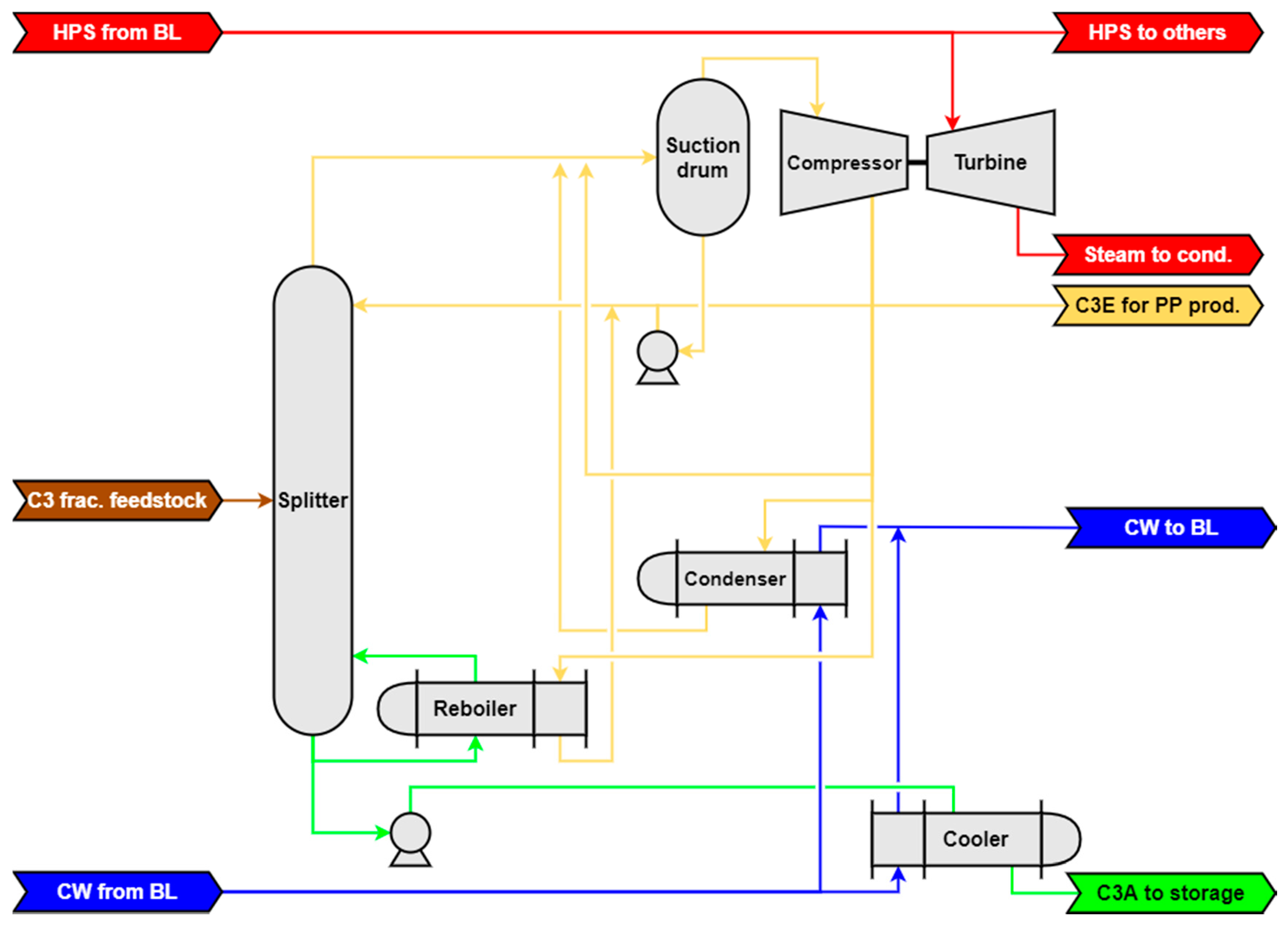
Process steam drives are important steam consumers in heavy industry [20,31,34] and play a significant role in the design and operation of complex steam networks. The most common driven equipment includes compressors, pumps, and fans (blowers) [34,38,47]. The steam turbines used can be of simple condensing, backpressure, or of a combined extraction condensing type [36]. Steam consumption is influenced by several factors that include the actual steam inlet parameters, steam discharge pressure, actual turbine revolutions, as well as the shaft work needed, which varies according to the process requirements. Process compressors driven by steam turbines are standard equipment of ethylene production and gas processing and fractionation plants [38,47], and they are also frequently used in compression heat pump-assisted distillations [48,49,50,51]. Thus, they are deeply integrated in the process. The shaft work needed depends on several process parameters, including (but not limited to) the distillation feed amount and composition, desired product quality, and column and compressor design parameters. This highlights the pressing need to develop a robust method for process steam drive sizing which would incorporate not only the real steam-side condition variations but also the process-side shaft work variations. Improper sizing results either in limited shaft work delivery (undersizing), causing possible process throughput limitations, or inefficient steam use (oversizing). Moreover, the steam drive design and operation have to be optimized with respect to the whole steam system, always taking into account the marginal steam source, its seasonal operation variations [52], and the possible steam pipeline capacity constraints [26,43].

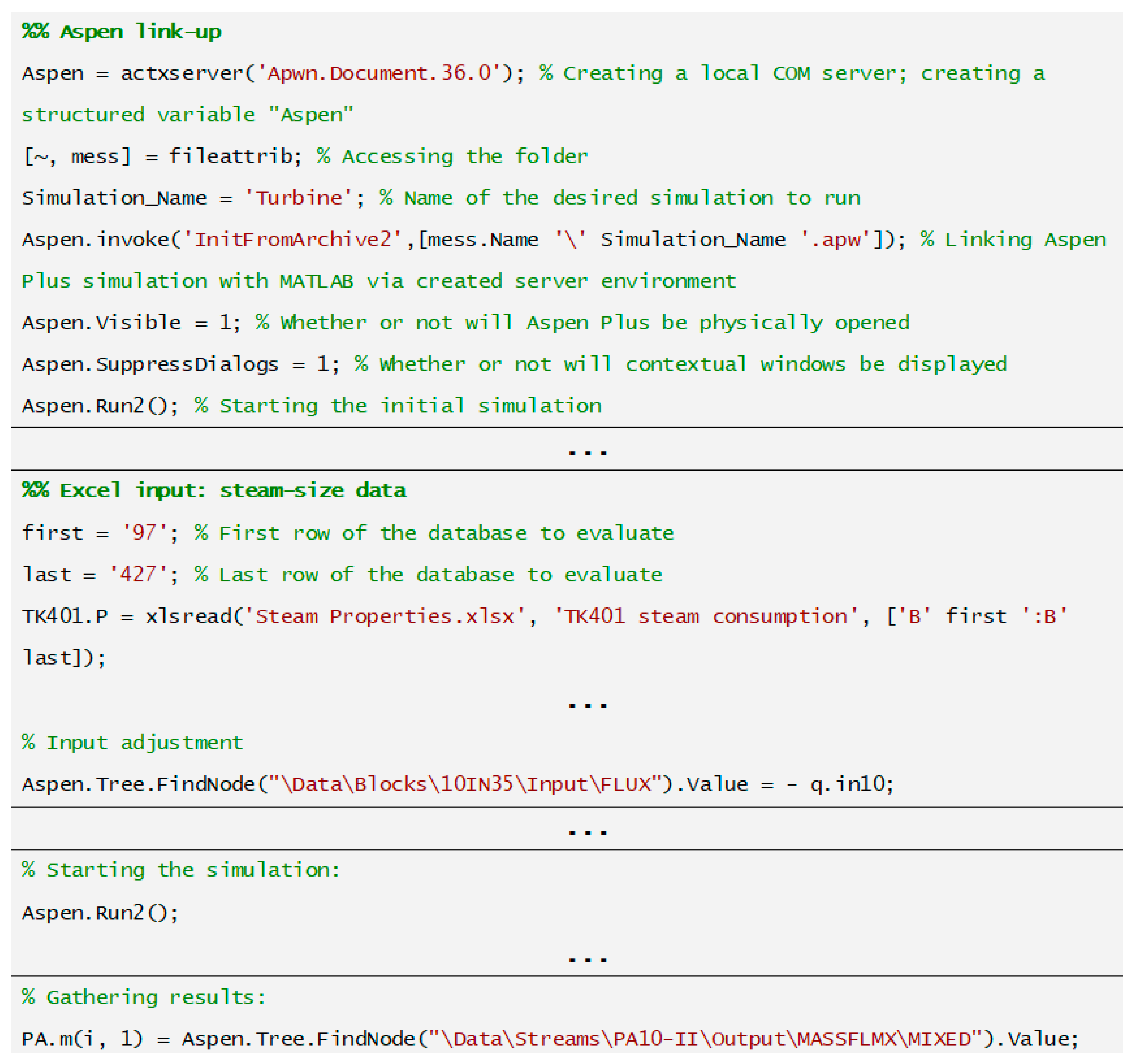
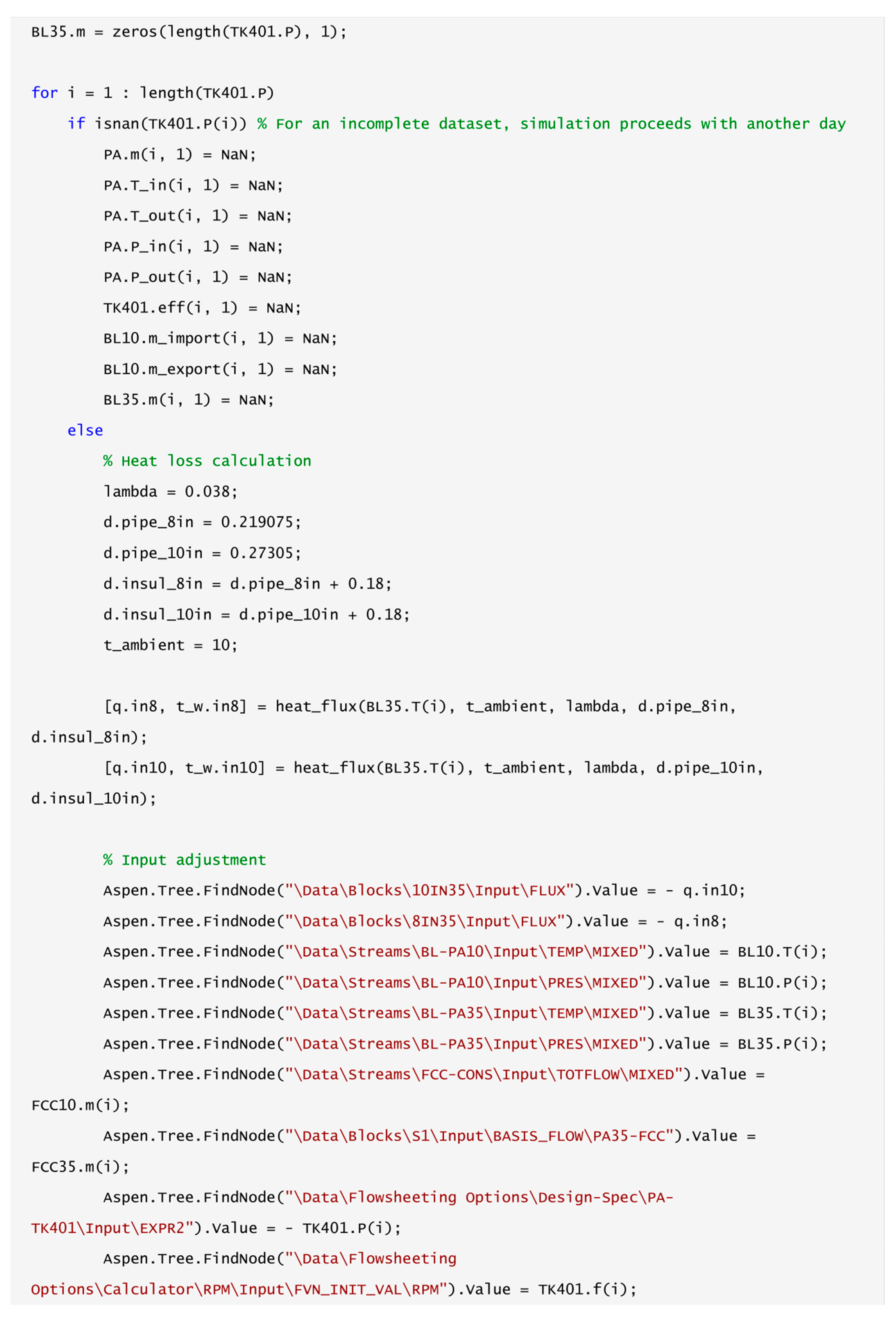
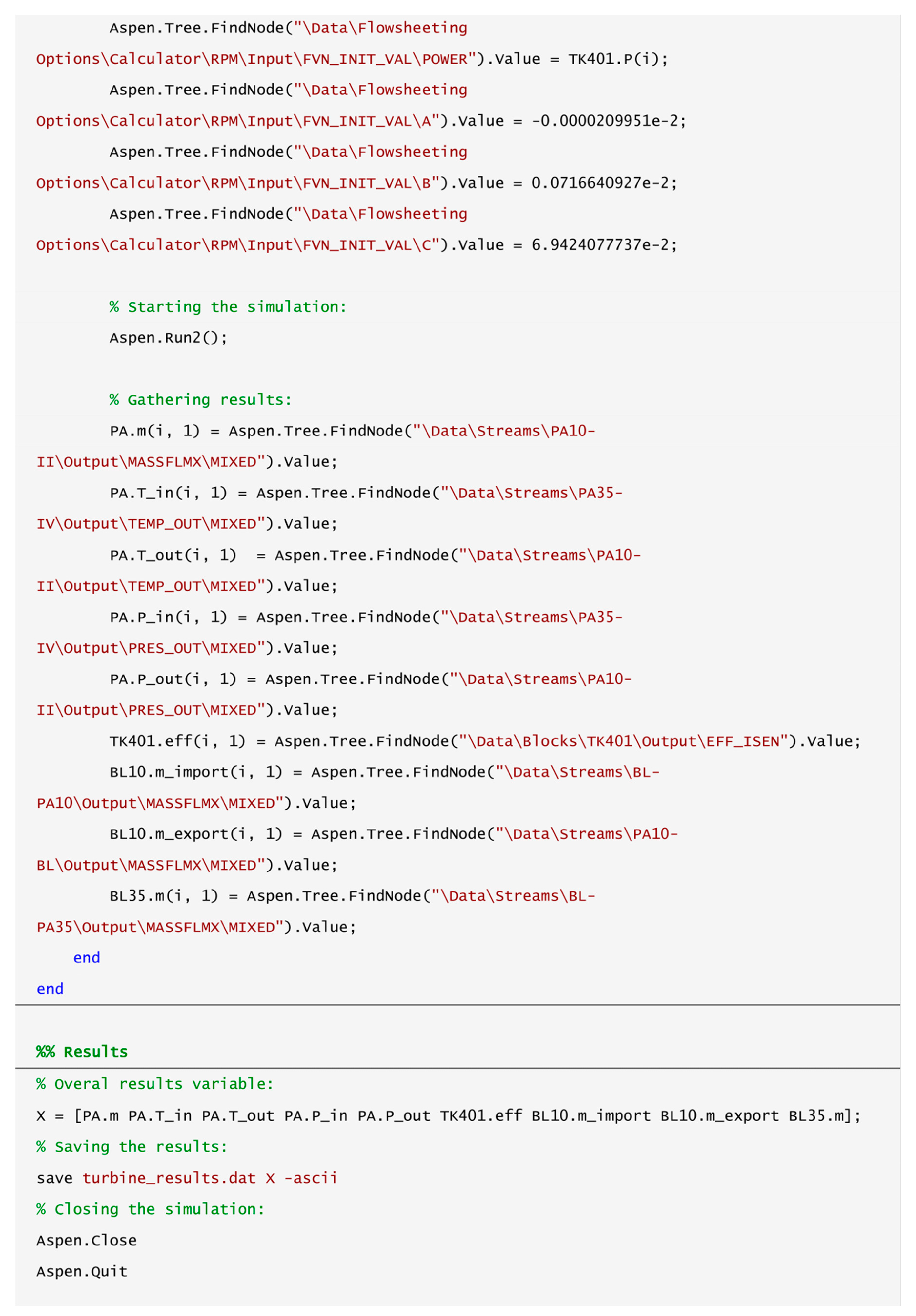
Given all the prerequisites, it is only natural that examination and precise evaluation of such complex process parameters poses a challenge which can hardly be faced successfully without employing robust simulation environment. For almost two decades, researchers have strived to combine the colossal computing capacity of the Aspen Plus^® simulation engine with the exceptional data-processing capabilities of the MATLAB^® software [53,54]. Several papers have been published, mostly focusing on multi-objective optimization [55,56,57,58,59] or automation problems solution [60,61]. Unfortunately, only scarce details regarding the chosen approach can be found. Hence, the perspective to close this gap in knowledge remains particularly attractive.

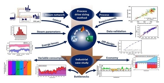
The contribution of this paper to the field of knowledge is twofold:

• First, it presents a robust method for optimal process drive sizing and integration considering all relevant factors affecting the design, while the method is suitable for operational optimization as well;
• Second, both the process-side and steam-side are modeled using Aspen Plus^® and MATLAB^® linking, which is a novel and promising approach for complex systems’ operation analysis and optimization purposes.

Table 1. Comparison of key parameters of the proposed method with recently published papers. Legend: BE = balance equations, Calc. = calculated, N/A = not applicable, NP = not provided, Reg. = calculated based on statistic regression, SA = sensitivity analysis, SS = saturated steam, WS = wet steam.

Parameter/Feature	Method
	Wu et al. [36]	Ng et al. [31]	Frate et al. [24]	Marton et al. 2017 [29]	Sun et al. 2016 [34]	Bütün et al. [43]	Mrzljak et al. [30]	Tian et al. [35]	Proposed Method
Inlet steam temperature & pressure	Fixed	Fixed	SS; SA	NP	SA	Fixed	Varying; process data	SS; SA	Varying; process data
Discharge steam pressure	Fixed	Fixed	SA	NP	NP	Fixed	Varying; process data	SA	Varying; process data
Discharge steam temperature	Fixed	Fixed	WS	NP	NP	Fixed	WS	WS	Calc.; polytropic expansion
Frictional pressure losses	🗶	🗶	🗶	🗶	🗶	🗸	🗶	🗸	🗸
Heat losses from pipelines	🗶	🗶	🗶	🗶	🗶	🗸	🗶	🗶	🗸
Turbine revolutions	🗶	🗶	🗶	🗶	Varying; NP	🗶	Varying	SA	Varying; process data
Turbine efficiency	Reg.	Fixed	SA	NP	Varying	NP	Calc.	Calc.	Calc.
Driven equipment efficiency	Fixed	N/A	N/A	N/A	Varying; NP	N/A	Efficiency map	N/A	Efficiency map
Shaft work required	Fixed	N/A	N/A	N/A	Calc.; process-dependent	N/A	Varying; process data	N/A	Calc.; process-dependent
Process modeled	🗶	N/A	N/A	Aspen utilities planner + Excel	Process and steam BE	Steam and heat BE	🗶	N/A	Aspen Plus® linked with MATLAB®

provides a comparison of the key parameters and characteristics of relevant recently published methods with the proposed method, all of them aiming at: 1. Maximization of the cogeneration potential exploitation; 2. optimal process steam drive sizing; and 3. optimal steam vs. electrodrive use. As is seen in Table 1, the relevant methods are focused mostly on steam-side modeling and optimization, while the proposed method presents a coupled steam- and process-side modeling approach. Moreover, several of the relevant methods do not incorporate such important aspects as the varying inlet steam parameters or shaft work requirements and implement fix turbine and driven equipment efficiencies instead of considering their variations in the real operation. As documented on an industrial case study, failure to implement the real operational parameters of a system leads to steam drive undersizing and, consequently, to limited process throughput.

The effect is that the more pronounced, the farther the process drive is located from the main steam pipeline. Further findings from the industrial case study include the fact that the incorporation of a steam drive into an existing steam network can significantly affect its balance (and, thus, its operation) and thus create a new operation bottleneck, or remedy its existing ones. Furthermore, the marginal steam source operation mode is also affected, which has to be considered when evaluating the economic feasibility of such an investment proposal.

Paper organization is as follows: Part 2 presents the proposed complex steam drive sizing method and is subdivided into process-side and steam-side model subparts. Following that, part 3 introduces an industrial case study with the description of the existing system layout, proposed change, available process data, and their processing, including initial analyses and their results serving as additional model input parameters. Part 4 presents the calculation results, including a comparison of the presented steam drive sizing method with several others (included in Table 1), and evaluating the economic feasibility of the proposed system change. Discussion is followed by a concise conclusion part summing up the novelty and significance of the presented method and the key findings extracted from the industrial case study results.

2. Process Drive Sizing Method

2.1. Equipment Operation Assessment and Modeling

2.1.1. Heat Pump-Assisted C3 Fraction Splitting

Heat pump-assisted distillation is a good example of incorporating a steam drive into an industrial process; thus, it was chosen for illustration. In such systems, overhead distillate vapors from a separation column are compressed and subsequently condensed in the column reboiler [51,62]. For this type of heat pump to be applicable, the separated components have to be of similar boiling points [63]. However, this leads to a relatively low driving force in the reboiler; thus, to deliver the required power input, the vapor throughput needs to be sufficiently high. Hence, stable operation of the heat pump compressor is of the uttermost importance. Amongst the compressor drives, steam drives (turbines) are the most usual. These are normally shaft-bound with the compressor and, therefore, their correct sizing is just as important as that of the compressor itself. In the case of steam turbines, however, the whole sizing process is more complicated as steam quality fluctuations and overall steam network properties have to be considered.

A typical arrangement of a heat pump-assisted distillation is provided in Figure 1. Here, a propane–propylene mixture is split into separate components of high purity (>99.6% vol.). The energy necessary for the separation is provided by a condensing steam turbine.

To design (size) a process drive correctly, the process itself must be understood thoroughly. This encompasses not only the physical structure of the system but also the physicochemical and mechanical non-idealities and, most importantly, over-time variations in feedstock quality and mass flow [64]. To provide the most authentic results, the model was constructed as follows:

• Due to simplicity of the mixture being distilled, an equilibrium model using Murphree tray efficiency was chosen;
• To account for the vapor phase non-ideality, the Peng–Robinson equation of state [65] was applied, as it yielded the best results compared to the measured data [66];
• Because the operating temperature of the column (25–35 °C) was similar to ambient temperature, heat loss from the system was neglected;
• Technical details regarding the number of column trays and the position of the feed stage; exchanger areas, overall heat transfer coefficients, and logarithmic mean temperature differences; and compressor and condensing turbine characteristics were taken from technical documentation provided by the manufacturer.

The model briefly described above was, due to its complexity, constructed in the simulation environment of the Aspen Plus^® software which provided fast-to-obtain and reliable results. Yadav et al. [67] provided a comprehensive tutorial on utilizing Aspen Plus^® potential in distillation column operation simulation. For the separation column, the RadFrac model was chosen, which stands as a universal rigorous model for multi-stage component separation. Each of the three heat exchangers was modeled using a short-cut method (HeatX model) which proved satisfactory for the cause. Both the compressor and the turbine were modeled using the Compr model [68,69], though individual approaches differed significantly.

2.1.2. Compressor Operation

In general, there is a variety of approaches regarding compressor modeling—from the simplest calculations (e.g., polytropic work calculation with constant parameters and efficiencies) to the most complex ones (comprising efficiency and power maps, and shaft speed calculations) [70,71]. As shown later, the calculation should be carried out in the most precise way possible whenever the data is accessible as, for instance, compressor shaft revolutions affect the turbine efficiency drastically. Hence, performance and efficiency curves were included in the model via the Aspen Plus^® interface. As a result, the model considered the mass flow through the compressor and the desired output pressure, and provided information on the required power input, polytropic efficiency, and shaft speed, as well as complete outlet stream results.

2.1.3. Process Drive Operation

Steam turbines, like compressors, can be modeled on many levels—from basic enthalpy balance with constant isentropic efficiency to more complex approaches comprising turbine characteristics and correction curves [20,30]. Aspen Plus^® did not provide the option to model turbines with the same precision as the compressors. Therefore, the characteristics and correction curves had to be input “manually”, via a calculator block. As only isentropic calculations were predefined for turbines, the model first calculated the turbine steam consumption based on the characteristics (required power output) and correction curves (live steam pressure, live steam temperature, exhaust pressure, and compressor revolutions). Then, the model iteratively calculated the isentropic efficiency of the turbine so that, based on the before-calculated steam consumption and enthalpy balance, the provided power output correlated with the required value.

2.1.4. Steam Network

While most industrial facilities have a major steam source (e.g., a combined heat and power unit (CHP)), the utilization of waste heat from production units in means of steam production is also a common practice [43]. Moreover, the overall steam supply of these local producers can even exceed the major steam source production. Thus, the quality of the supplied steam varies significantly depending not only on the CHP unit’s operation but on the whole production network [22,72]. It is therefore vital for process drive sizing to account for steam quality fluctuations.

When analyzing steam networks, as well as any other pipeline systems, momentum and heat transfer must always be considered [73]. Pressure loss caused by friction and/or various installed armatures and potential heat loss to ambient space can affect the steam quality significantly. When analyzing the heat transfer, steam–ambient temperature difference plays the most significant role. The impact of heat loss on the medium quality is thus best observable during extreme ambient conditions, i.e., temperature peaks during winter. Even though most adverse effects of ambient temperature changes can be suppressed by effective insulation, Hanus et al. [26] showed that the effectivity of outdoor insulation decreases heavily after years of operation and it is in designer’s best interest to investigate the true heat conductivity of the used insulation.

Effects of both pressure and heat losses vary greatly depending on pipeline geometry and mostly on the steam network topology and plant infrastructure, i.e., the resulting pipeline length. While the distance (pipe length) of the considered steam drive from the battery limit header can range in terms of tens of meters in some cases, there are units where the pipe length can reach hundreds of meters or even a kilometer. This is mostly the case of mid-twenty century refineries where individual units and their subunits were built far apart for safety reasons [26].

Lastly, it is necessary to assess the impact of steam drive alteration on the steam transport velocity. Naturally, high transport velocities may cause serious erosion of pipeline walls and damage installed armatures. However, low velocities in the pipelines may result in excessive heat loss and decrease in steam quality or even condensate production [26]. Hence, the velocity changes with the steam consumption of the drive, and pipeline suitability assessment is inevitable.

The process described in the previous text draws high-pressure steam from a steam network using a CHP unit as the main steam producer. As illustrated below (Figure 2), steam crossing the fluid catalytic cracking (FCC) unit battery limit is first supplied to the modeled system (propylene recovery unit) and then to other parts of the FCC unit. To account for all above-mentioned aspects, pipeline topology, geometry, and heat transfer properties were incorporated in the Aspen Plus^® process model.

2.1.5. Combined Heat and Power Unit (CHP) as Marginal Steam Source

Industrial combined heat and power plants (CHP) traditionally employ steam boilers and steam turbines as the cogeneration technology; some of them including gas turbines or combustion engines [40,74]. Their task is to cover the steam network imbalance on all pressure levels (i.e., to serve as a marginal steam source) while the cogenerated electric energy is utilized in the industrial facility or sold to an external grid. Seasonal steam demand variations influence their operation and the resulting backpressure power production decreases in summer below a pre-set acceptable level, and has to be compensated by other means (condensing power production). The reason for this specific system feature is explained in more detail in Section 3.2. Techno-economic assessment of a process steam drive sizing inevitably impacts the CHP operation and should be evaluated correctly. Last, but not least, the CHP operation is influenced not only by internal steam demand, but by external factors as well (energy management strategy of the refinery, changeable energy prices and their uncertainty, etc.) [75].

The considered CHP comprised high-pressure steam boilers (9 MPa, 530 °C) and a set of backpressure and extraction condensing turbines exporting high-pressure (HPS, 3.5 MPa), medium-pressure (MPS, 1.1 MPa), and low-pressure (LPS, 0.5 MPa) steam to the industrial facility. Constant marginal heat production efficiency of the CHP and constant marginal backpressure and condensing power production per one ton of steam were assumed. The effect of a change in the production unit steam balance on a certain pressure level was transposed to the corresponding change in backpressure electric energy production and fuel consumption in the CHP. A detailed description of the CHP unit operation and its further characteristics can be found elsewhere [26,47].

2.2. Data Processing

Data analyses are an inherent part of any technological proposal. To be able to size the desired equipment, it is necessary to understand the unit’s operation, unearth any possible off-design performance and to map the system responses. In order to do so, measured data regarding the modeled unit and auxiliaries have to be studied.

To evaluate the maximal power requirements of the modeled unit and to assess seasonal performance variations, a year-long operation of the unit was monitored. To understand the effects of steam quality fluctuations on the proposed new process drive performance, daily measurements of the properties of steam in the network were taken. Finally, to examine possible bottlenecks linked to the CHP unit operation, its performance during the evaluated period was considered.

2.2.1. Measured Data

Table 2. Considered measured data. Legend: BL = battery limit, CHP = combined heat and power plant, HPS = high-pressure steam, MPS = middle-pressure steam.

Equipment/Material Stream/Unit	Data	Purpose	Details
Propylene (product stream)	Total mass flow	Simulation	Together with propane stream represents the feed stream
	Propylene content
Propane (component analysis)	Simulation	Feed stream composition
Column	Head pressure	Simulation
	Bottoms pressure	Simulation
Suction drum	Pressure	Simulation
Compressor	Exhaust pressure	Simulation
	Exhaust temperature	Verification	Compressor exhaust temperature documents isentropic efficiency calculation accuracy
	Shaft speed	Verification	Shaft speed documents compressor performance calculation accuracy
Turbine	Steam consumption/condensate mass flow	Verification	For systems where steam consumption is not measured directly, it is possible to measure mass flow of turbine condensate
	Condensate pump by-pass valve position	Verification	When measuring condensate mass flow, it is sensible to check whether condensate pump by-pass is in operation and to what degree
	Live steam temperature	Simulation
	Exhaust pressure/condenser temperature	Simulation	For systems where exhaust pressure is not measured directly, it is possible to estimate it based on the condenser temperature
HPS from BL	Mass flow	Simulation
(utility stream)	Temperature	Simulation
	Pressure	Simulation
MPS from BL	Mass flow	Simulation
(utility stream)	Temperature	Simulation
	Pressure	Simulation
CHP unit	HPS mass flow	Simulation
	MPS mass flow	Simulation

summarizes all process data used in the simulation of the propylene recovery unit performance and serves as a guide for heat pump-assisted distillation simulation (and process drive sizing) data gathering. These data include feedstock mass flow and composition which are usually not measured continually. However, highly reliable records of products’ mass flow and quality are generally recorded and they can be combined to obtain the desired information.

2.2.2. Aspen–MATLAB Linking

The proposed methodology exploits the full potential and relevance of multi-software modeling via linking Aspen Plus^® software (Aspen Plus^® V10, Aspen Technology Inc., Bedford, MA, USA) with MATLAB^® software (MATLAB^® 2020a, The MathWorks Inc., Natick, MA, USA). While the state-of-the-art simulation engine of Aspen Plus^® provides swift and rigorous results due to the sequential modular algorithm, its use in evaluation of large datasets containing numerous different variables is somewhat laborious. On the other hand, the programming language of the MATLAB software is tailored for handling such tasks. Thus, an effort to link these two software environments persists. Fontalvo et al. [54] introduced the idea of software linking in the early 2000s, though no details were presented. Several years later, in 2014, Fontalvo described the linking principles [53]; however, these are of limited relevance today. Other authors have continued working on the idea with different aims or providing insufficient details. A MATLAB^® sub-software, Simulink, was used by Dos Santos Vidal et al. [60] and Ryu et al. [61] to solve rather complicated automation problems. Muñoz et al. [57] used MATLAB^®-to-Aspen linking in a gradient-based multi-objective optimization via ACSII file exchange with Aspen Plus^® working in the equation-oriented mode. The published freeware by Abril [76] caused a breakthrough with instructions for component object model (COM) interface linking. Following this publication, several papers [58,59,77,78] were published providing scarce information about the interface build and utilization. Even though the works of Ramirez et al. [56] and Darkwah et al. [55] contain specific programming tips, these are rather unclear to a non-advanced user. Hence, to this day, a simple but complex interface linking methodology remains elusive. Details regarding the program capabilities and the linking procedure are presented in the following text.

Aspen Plus^® cooperation with external Windows applications is enabled via ActiveX Automation Server. In this way, the applications can interact with Aspen Plus^® through a programming interface while the automation server exposes objects through the COM object model [79]. Through this interface it is possible:

• to connect inputs and results of Aspen Plus^® simulations to other applications;
• to manipulate (create, reconnect, delete, etc.) Aspen Plus^® objects;
• to control the Aspen Plus^® user interface (handle events, suppress dialog boxes, disable user interface features, etc.);
• to control a simulation (run, stop, reinitialize, etc.).

As the original user guide for Aspen Plus^® is written for the Visual Basic programming language, a simple step-by-step manual for Aspen–MATLAB linking is presented:

• First, a local ActiveX server is created where the component object model is situated using the inbuilt function “actxserver”. The syntax is as follows: var = actxserver(ProgID), where var is a structured variable used to access the server and ProgID is the program identifier. The program identifier for Aspen Plus^® documents is “Apwn.Document.X” where X depends on the Aspen Plus^® version: 34.0 for V8.8, 35.0 for V9.0, and 36.0 for V10.0 (e.g., “Apwn.Document.36.0” for Aspen Plus^® V10);
• After the server creation, the whole system is initialized as shown in Figure 3. There are three initialization methods depending on the format of the simulation: “InitFromArchive2” (for use with .bkp and .apw archive files), “InitFromTemplate2” (for use with templates), and “InitFromFile2” (for use with .apwn compound files). No difference has been observed in their performance, though .bkp files are generally the smallest in size and thus recommended. As with other MATLAB^® scripts, all files have to be located in the same folder;
• From this point on, the Aspen–MATLAB^® link is ready to use. To access results, manage inputs, and control the simulation and/or the user interface, dot notations are used. Examples of the syntax for various commands are given below:
  • Simulation control
    Syntax: var.command (e.g., var.Run2, var.Reinit, …)
  • User interface control
    Syntax: var.attribute = value (e.g., var.Visible = 1, …)
  • Input alteration
    Syntax: var.Tree.Findnode(path).Value = value_a
  • Results gathering
    Syntax: value_b = var.Tree.Findnode(path).Value

All commands can be found in Appendix A or in Figure 3. The path to every individual variable of the simulation in Aspen Plus^® can be accessed directly in the program via: Customize→Variable explorer.

• Prior to launching the simulation, it is sensible to also link MATLAB to Excel for more flexible operation via simple and useful inbuilt functions “xlsread” and “xlswrite” enabling reading and writing data from and to the Excel spreadsheet, respectively, without the need for opening the data file manually. An example can be seen in Figure 3.

3. Industrial Case Study

3.1. System Description

The aforementioned propylene recovery unit is a subunit (a section) of a fluid catalytic cracking (FCC) unit, splitting the liquid propylene–propane fraction from the FCC gas plant into individual products of high purity. Due to low relative volatility of the components (and therefore low temperature difference between the head and bottom of the distillation column), a compression heat pump system can be utilized. However, the small difference in boiling points demands a large reflux ratio (>15) and numerous (>150) separation stages. Hence, such a system (as described in Figure 1) poses not only a technological but also a computational challenge, which once again underlines the pressing need for use of robust simulation software.

Performance of the considered propylene recovery unit was evaluated during an approximately one-year period, from 1 April 2018 to 28 February 2019, and provided the following observations:

• The unit’s feedstock flow rate was flexible, ranging from 6.5 to 9.7 t/h;
• Feedstock quality ranged from 81.7 to 86.5 mass % of propylene;
• Turbine condensate pump was by-pass protected.

Based on the technical documentation, we can state:

• Maximal unit throughput was 10 t/h of the propane–propylene fraction;
• Maximal compressor power at the coupling is 1250 kW.

3.2. Proposed Change in Steam Drive Type

Currently, a condensing steam turbine is used as the heat pump compressor drive. Such a situation makes sense if there is excess steam that cannot be utilized for other purposes (process heating, stripping agent, etc.). In the presented industrial study, HPS, used as driving steam, was imported from the CHP. At the same time, enough variability in both HPS and MPS production and transport capacities allowed us to consider condensing steam drive replacement by a backpressure one, targeting fuel savings in the CHP at the expense of a certain loss of CHP power generation. The replacement of condensing mechanical power production by a backpressure unit is economically feasible at most fuel-power price ratios. An additional tangible benefit was the resulting decrease in CO₂ and other pollutant emissions in the CHP.

Another steam pressure level, LPS, can be considered as an alternative backpressure steam sink to the MPS, but it is less suitable for this purpose. The reason is an occasional LPS excess in summer and the resulting decrease of LPS export from the CHP to very low values, which negatively affects the steam quality in the main LPS pipelines. Additional LPS from a new backpressure steam drive would thus have to be vented into the atmosphere. This situation is well-documented in Figure 4, where occasional drops of LPS export from the CHP can be seen. Sudden one-direction changes in LPS export within a few days or one to two weeks (decrease in April, increase in November) result from switching on/off the space heaters and steam tracing in the refinery. The existing LPS excess in the refinery during summer months is a serious issue that has two consequences: First, lower economic attractiveness of incentives for LPS consumption decrease in the refinery. Second, low LPS export from the CHP leads to reduced backpressure power production. Long-term energy policy of the refinery includes the demand to secure the power supply to critical production units during outer grid outages (severe weather, unexpected events) from the CHP. Thus, a certain minimal power production in the CHP is required regardless of the actual season. As the backpressure power production is insufficient to cover this demand, additional power is produced in condensing steam turbines during warmer months. The average duration of this period is 40% of the year. Any changes in CHP backpressure power production resulting from the proposed change in the steam drive are reflected in the change of condensing power production in the opposite way during this period of the year.

Apart from MPS and LPS, other steam pressure levels can be considered with sufficient capacity to absorb the steam produced from the new steam drive. A preliminary analysis of steam consumption in the FCC unit showed no such options, as their steam absorption capacity was only a small fraction of what was needed. Thus, only a backpressure steam drive with HPS as the driving steam and with MPS discharge was considered and further analyzed. A schematic of the analyzed proposal is provided in Figure 5. The FCC unit consumed between 25 to 40 t/h of MPS. During periods of lower MPS consumption, the excess of MPS produced in the new steam drive was exported to other refinery units. The CHP remained the marginal source of both HPS and MPS for the refinery. MPS export from the FCC unit was associated with increased MPS backpressure at the new steam drive discharge, which was considered in the proposed steam drive sizing method. Increase in the HPS export from the CHP increased the steam flow velocities in the HPS network, which was desirable following the outcomes of a study dedicated to HPS network operation [26]. However, transport capacity of both main HPS pipelines as well as those within the FCC unit has to be reviewed.

3.3. Key System Analysis and Model Verification

Prior to designing a new process equipment, it is inevitable to confirm the relevance of the constructed model, based on which the proposal will be carried out. Designing a new process steam drive, the best practice is to prove that the model can predict actual steam consumption precisely. According to the enclosed graph (Figure 6), the model prediction seems to be incorrect though the trend is generally preserved. This was probably caused by the lack of live steam consumption measurement, except for the turbine condensate mass flow, which did not, however, totally correlate with the steam consumption because of the condensate pump by-pass increasing the condensate flow. Moreover, as shown in Figure 7, the calculated compressor shaft speed was in most cases slightly lower than the measured one due to the applied process control: For systems comprising such an enormous recycle stream flow rate (>150 t/h recycle vs. <10 t/h feedstock) it was near impossible to numerically obtain the exact same composition as analytically determined. Rather than that, an automation condition was set, forcing the process control to keep the product quality above 99.6 vol%. Even though real process control can occasionally achieve higher purity, there were numerous cases where the calculated purity was slightly below the measured. As a result, the compressor shaft speed may have, on a small scale, differed from the measured as well.

To account for both effects, the condensate mass flow rate with by-pass valve position was included in the calculation and the measured shaft speed was used for turbine performance assessment. The latter perfectly illustrated the impact of the shaft speed on the turbine efficiency (discussed in detail later). Based on the measured to calculated condensate mass flow rate comparison (Figure 8 and Figure 9), it can be stated that the model provided reliable results and was thus verified.

Subsequently, to design a process drive correctly, it is necessary to:

• Obtain the process side characteristics—to evaluate the maximal power requirements and predict the process behavior in case of insufficient power supply as well as the daily performance;
• Map fluctuations in the steam network as to find the most appropriate design parameters for a new steam drive;
• Understand the effects of the process side (shaft speed and power requirements) and steam side (live steam pressure, live steam temperature, and exhaust pressure) parameters on turbine efficiency.

Considering the above, process side characteristics (Figure 10) were constructed. Despite expectations, the primary assumption that the feedstock quality affects the process side power requirements was refuted. The best explanation was that the impact of large reflux efficiently suppressed the impact of the feedstock quality and so the characteristics were practically linear, with the feed flow rate as the independent and the power requirement as the dependent variable. The slope of the linear function used to fit the data was later used in results.

The installed condensing steam turbine provided 1250 kW of power at nominal conditions, i.e., live steam pressure of 2.95 MPa, live steam temperature of 300 °C, exhaust pressure of 25 kPa, and shaft speed of 11,548 rpm, while consuming 2.1 kg/s of HPS. At these conditions, isentropic efficiency of 71.9% was declared. Based on the enclosed technical documentation (correction curves), the effect of alteration of these parameters was studied. The results can be observed in the figures below. It was proven that steam side parameters (Figure 11) affect the turbine isentropic efficiency insignificantly, as even the highest relative parameter deviations caused no more than a 2% difference in isentropic efficiency. Moreover, it is worth mentioning that no such drastic deviations occur in real steam networks, and thus the impact of steam side parameters on the isentropic efficiency can be neglected. However, as it is shown below, the shaft speed affected the isentropic efficiency to a high measure, while a change in shaft speed was a common phenomenon resulting from variations in the system performance and the feedstock throughput. Hence, the effect of shaft speed alteration on turbine isentropic efficiency was normalized (Figure 12) for designing the new turbine.

The study of actual steam side parameters, however, showed that the installed turbine operates off design as the real steam network measured values differ from the nominal ones. Hence, the parameters measured at the FCC unit battery limit were displayed in histograms (Figure 13, Figure 14, Figure 15 and Figure 16) to obtain ideal design parameters for the new steam drive.

Temperature and heat losses were studied on a plant-wide scale. Measured values of temperature and pressure of HPS exported from CHP were compared to those measured at the FCC battery limit. The results can be seen in Figure 17. Rather significant differences can be observed namely in temperatures where an almost 50 °C decrease was documented. These results illustrate the need for pressure and heat loss assessment prior to any proposals incorporating steam networks.

3.4. Variable Approaches in Steam Drive Design

The steam turbine model was based on steam turbine characteristics well known as the Willan’s line [80,81], i.e., linear dependency of the actual turbine’s shaft output, $P$, on the actual steam mass flow, $\dot{m}$, Equation (1), applied to steam expansion between HPS and MPS, with $I$ being the intercept of the linear relationship:

$$P=k\dot{m}-I$$

(1)

As reported by Mavromatis and Kokossis [80], the slope, $k$, in Equation (1) can be expressed as follows, in Equation (2):

$$k=\frac{1.2}{B}\left(\Delta h_{IS}-\frac{A}{{\dot{m}}_{max}}\right)$$

(2)

Parameters A and B can be correlated as a function of inlet steam saturation temperature (see [80] for further details); $\Delta h_{IS}$ represents the isentropic enthalpy difference between inlet and discharge steam, depending on the inlet steam pressure and temperature as well as on the discharge pressure; ${\dot{m}}_{max}$ stands for the maximal (design) steam mass flow through the turbine. As verified in [47], values of k for common steam drive applications do not differ significantly from $\Delta h_{IS}$ and, thus, $\Delta h_{IS}$ is used as the slope of the steam drive characteristics in the steam turbine model. Once the nominal turbine steam consumption, the nominal obtained output, and the slope of the characteristics are known, the steam turbine characteristics can be constructed. Following the engineering practice of steam turbine vendors, when depicting the given relationship, the inlet steam mass flow is located on the y-axis and the obtained output on the x-axis. Thus, an inverse function to Equation (1) is depicted in Figure 18, with its slope being equal to ${\Delta h_{IS}}^{-1}$, as seen in Equation (3):

$${\dot{m}}_s = \frac{1}{\Delta h_{IS}}P + \frac{I}{\Delta h_{IS}} = \frac{1}{\Delta h_{IS}}P + K$$

(3)

Varying inlet steam conditions and discharge pressure impact the $\Delta h_{IS}$ value and thereby affect the actual turbine’s steam consumption necessary to achieve the desired output. The analysis of process side characteristics revealed the maximum power requirement of 1278 kW to be supplied by the turbine. For the new turbine, the design power output was thus set to 1300 kW. According to numerous publications on isentropic efficiency of industrial steam drives [30,82], an isentropic efficiency of 65% was assumed, which is typical for mid-size industrial steam drives operating at full load with a low-steam pressure ratio. Mechanical efficiency of such equipment can be estimated to be 85% [81]. While the mechanical efficiency changed in a very short interval and thus could be considered constant for a reasonable operational window [81], the isentropic efficiently changed significantly regarding the turbine load. The dependence between turbine power and isentropic efficiency has been well documented before [80]. It can be calculated directly from the Willan’s line and described in the form of a parabolic function (Figure 19).

To find the design point and subsequently construct the turbine characteristics, several approaches are available (Table 1). These vary depending on the number of variables considered, i.e., on the number of system properties that are neglected and/or simplified. To provide a comprehensive overview, a variety of possible approaches was exploited to illustrate the main differences in the resulting design (

Table 3. Steam drive design approach variations. Real insulation conductivity of 0.080 W·m⁻¹·K⁻¹, calculated previously by Hanus, et al. [26], was considered. Design insulation conductivity of 0.038 W·m⁻¹·K⁻¹ was considered as a common value for new steam pipeline insulations.

Approach	Pipe Length	Pipeline Heat Loss		Pressure Drop	Steam Quality Fluctuations	Varying Shaft Speed	Varying Isentropic Efficiency
		Real Insulation Conductivity	Design Insulation Conductivity
Case 1	100%	🗸	🗶	🗸	🗸	🗸	🗸
Case 2	100%	🗶	🗸	🗸	🗸	🗸	🗸
Case 3	100%	🗶	🗶	🗸	🗸	🗸	🗸
Case 4	-	🗶	🗶	🗶	🗸	🗸	🗸
Case 5	-	🗶	🗶	🗶	🗶	🗸	🗸
Case 6	-	🗶	🗶	🗶	🗶	🗶	🗸
Case 7	1000%	🗸	🗶	🗸	🗸	🗸	🗸
Case 8	1000%	🗶	🗸	🗸	🗸	🗸	🗸
Case 9	1000%	🗶	🗶	🗸	🗸	🗸	🗸
Case 10	-	🗶	🗶	🗶	🗶	🗶	🗶

). These cases were subdivided into three groups: Cases 1–6 considered the properties and topology of the existing propylene recovery unit, with only cases 1–3 considering the features of the pipeline; cases 7–9 illustrated the changes in results for a steam drive located ten times farther (in means of pipeline length) from the battery limit; and case 10 was a standalone case considering only the basic enthalpy balance and constant values of all parameters.

Pressure drop calculations for each segment of the pipeline came from the Bernoulli’s equation, which can be generally written as Equation (4):

$$z_{1}g+\frac{w_1^2}{2{\alpha }_1}+\frac{P_1}{\rho }=z_{2}g+\frac{w_2^2}{2{\alpha }_2}+\frac{P_2}{\rho }+{\epsilon }_{dis}$$

(4)

where $z$ is the geodetic height, $g$ the gravitational acceleration, $w$ the mean steam transport velocity, $P$ absolute pressure, $\rho$ fluid density, ${\epsilon }_{dis}$ specific dissipated energy, and the dimensionless parameter, $\alpha$, has the value of 0.5 or 1 for laminar or turbulent flow, respectively. Subscripts 1 and 2 refer to inlet and outlet of the pipe segment, respectively. For each segment, the inner pipe diameter remained constant. Thus, based on the continuity equation, the transport velocity remained constant as well. Furthermore, the difference in geodetic heights can be sensibly neglected and Equation (4) can be transformed into Equation (5):

$$\Delta P=\rho {\epsilon }_{dis}$$

(5)

The overall specific dissipated energy comprises dissipation due to friction and local energy dissipation. Based on the Darcy’s law, Equation (6) is deduced:

$$\Delta P=\rho \left(\lambda \frac{L{w}^2}{2D}+{{\displaystyle \sum }}^{}\xi \frac{w^2}{2}\right)$$

(6)

where $\lambda$ is the friction factor, $L$ the length of the pipeline segment, $D$ the inner diameter of the pipeline segment, and $\xi$ is the coefficient of local dissipation. A generalized ready-to-use approach for friction factor estimation was proposed by Brkić and Praks [83].

Assuming that the only significant heat transfer resistances are that of the insulation and that of the ambient space, the following Equations (7) and (8) apply:

$$T_F\approx T_W$$

(7)

$${\dot{q}}_L=\frac{\pi \left(T_F-T_I\right)}{\frac{1}{2\kappa }\ln \frac{D_I}{D_W}}=\frac{\pi \left(T_F-T_A\right)}{\frac{1}{2\kappa }\ln \frac{D_I}{D_W}+\frac{1}{{\alpha }_A{D}_I}}$$

(8)

where $T_F$ is the temperature of transported fluid, $T_W$ temperature of outer pipeline wall, $T_I$ the outer temperature of insulation, $T_A$ the ambient temperature, ${\dot{q}}_L$ the length-specific heat flux, $\kappa$ the heat conductivity of the insulation, $D_W$ the outer diameter of the pipe, $D_I$ the outer diameter including insulation, and ${\alpha }_A$ is the combined radiation and convective heat transfer coefficient.

Therefore, the length-specific heat loss from a segment can be iteratively calculated for $f=0$ from Equations (9)–(12) [84]:

$${\alpha }_A=9.74+0.07\left(T_{I,1}-T_A\right)$$

(9)

$${\dot{q}}_L=\frac{\pi \left(T_F-T_A\right)}{\frac{1}{2\kappa }\ln \frac{D_I}{D_W}+\frac{1}{{\alpha }_A{D}_I}}$$

(10)

$$T_{I,2}=T_F-q\frac{\ln \frac{D_I}{D_W}}{2\pi \kappa }$$

(11)

$$f=T_{W,2}-T_{W,1}$$

(12)

where $T_{W,1}$ is the primary estimate of the temperature of the pipeline wall (under insulation).

4. Results and Discussion

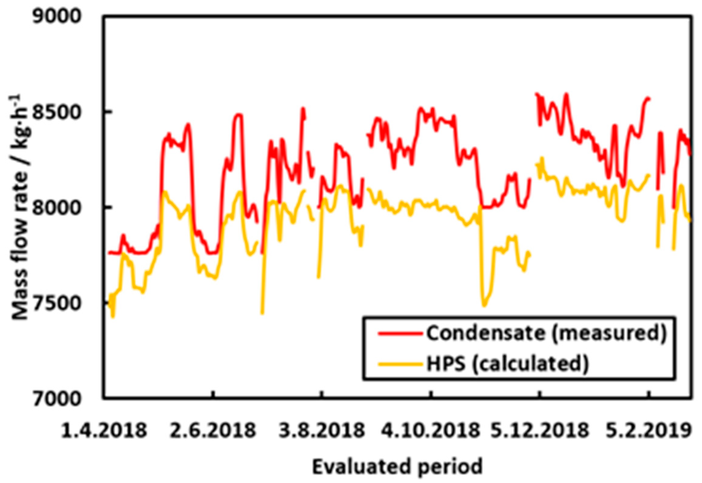
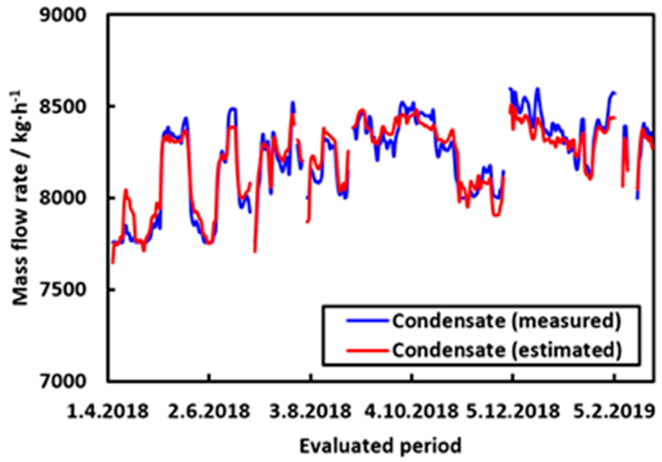
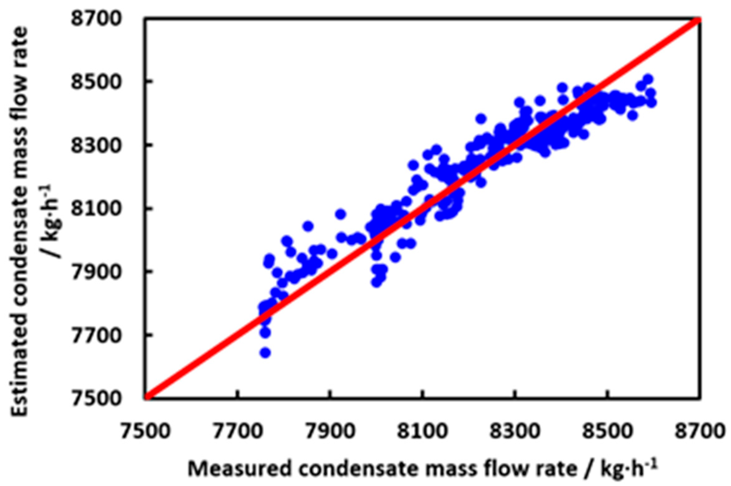
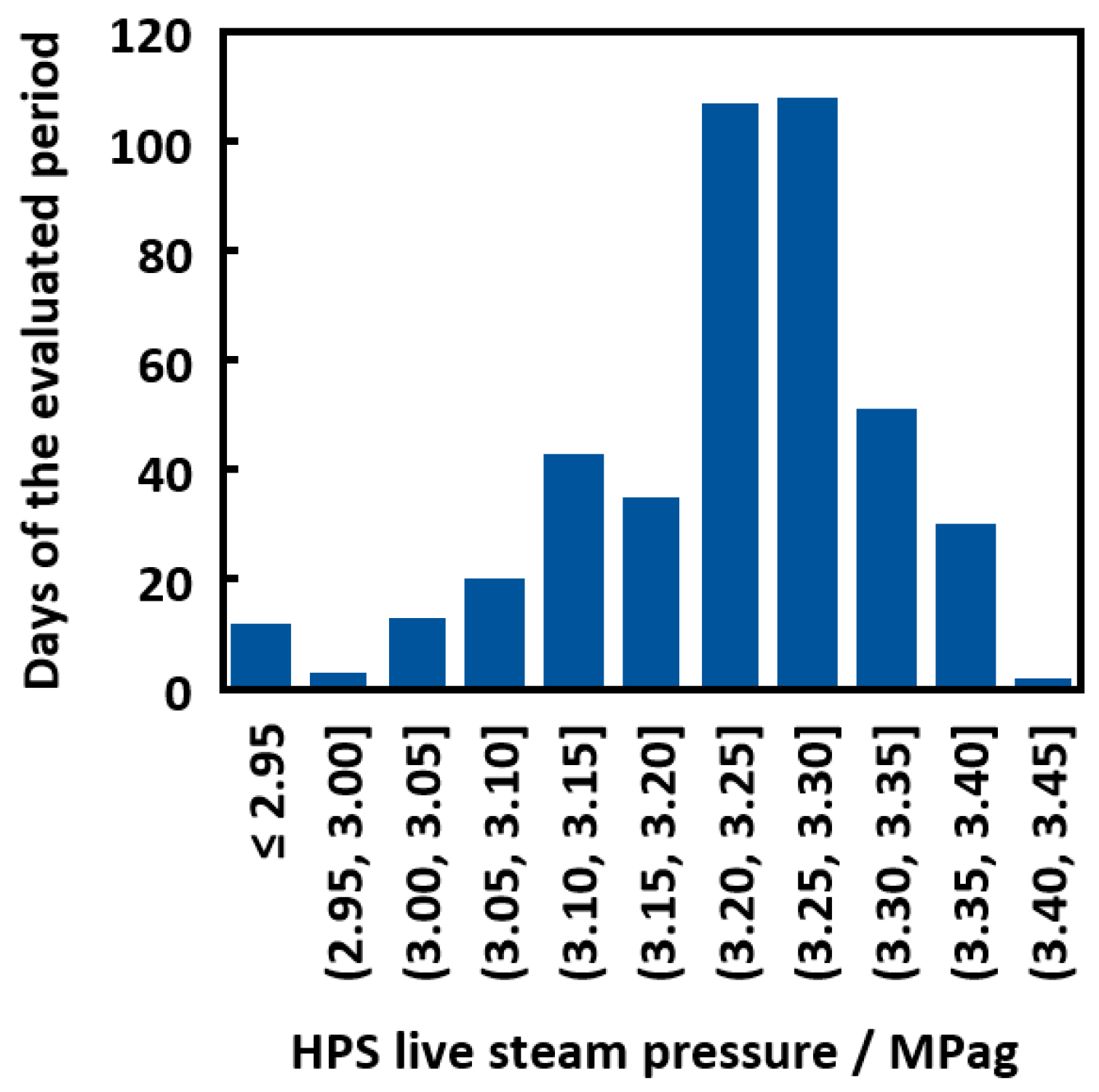
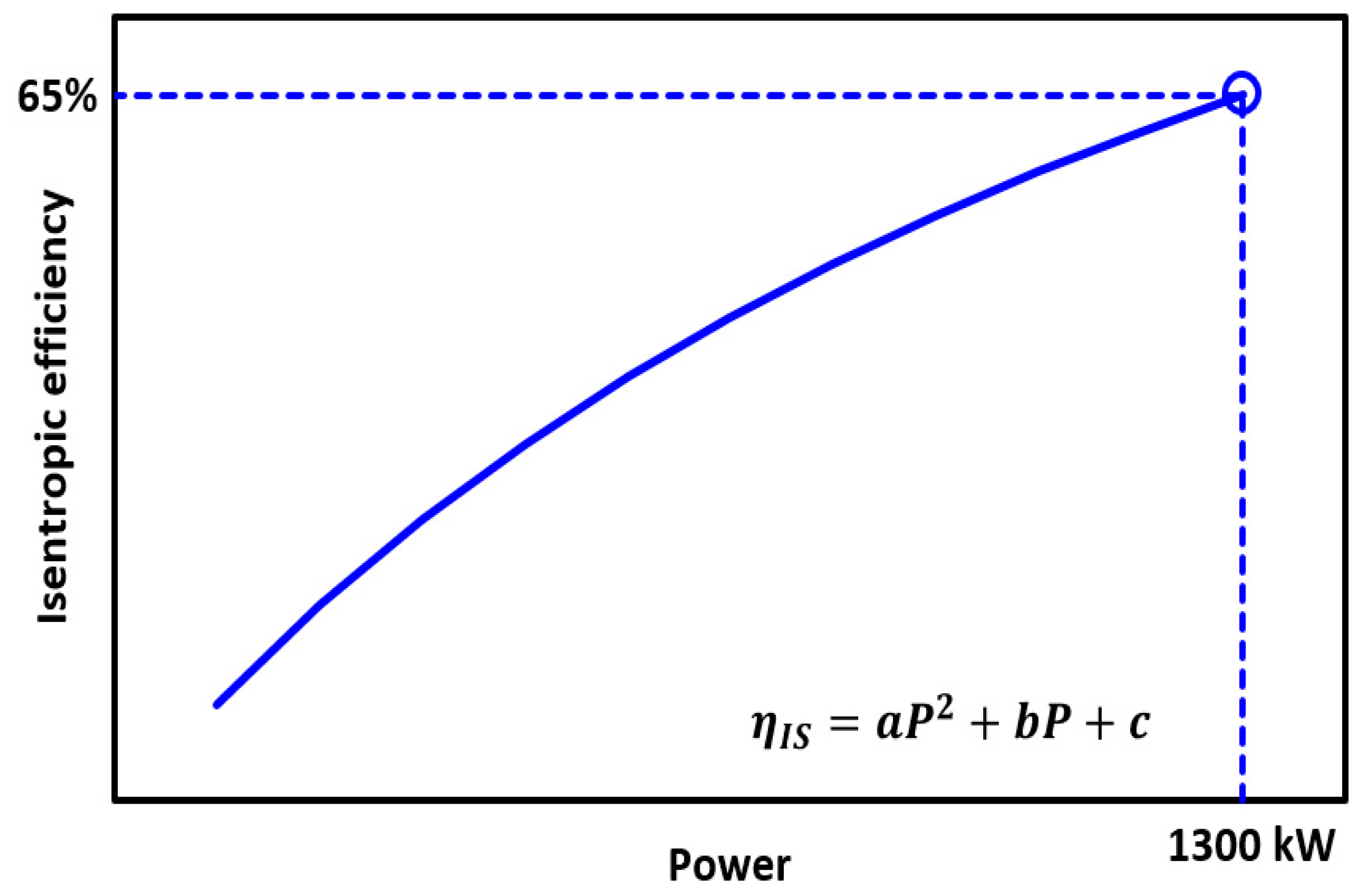
The proposed change in the process steam drive from the actual condensing steam turbine to a new backpressure one anticipated a significant increase in HPS consumption. Whereas the actual consumption ranged roughly from 7.5 to 8.5 t/h (Figure 6), preliminary calculations for the turbine at nominal conditions (3.35 MPa, 325 °C HPS (BL), 1.0 MPa, 252 °C MPS (BL), 65% isentropic efficiency, 85% mechanical efficiency, 100% compressor shaft speed) revealed an increase in turbine HPS consumption to approx. 35 t/h. 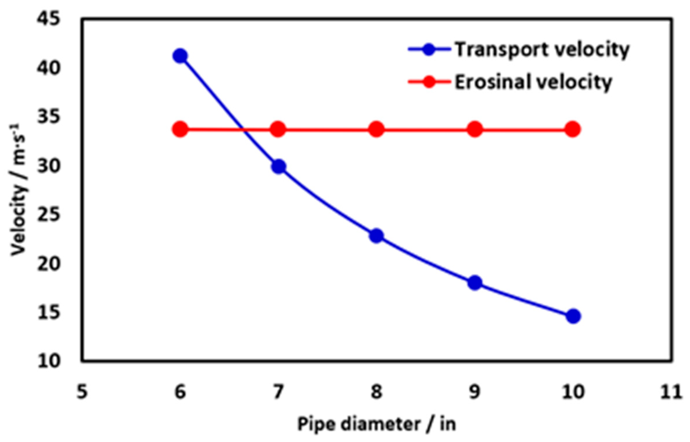Hence, steam transport velocities in the interconnecting pipeline were studied (Figure 20).

As the conducted case study showed (Figure 20), steam transported by a pipeline with a diameter below 7′′ would breach the erosional velocity limit defined for HPS. Thus, a pipeline with such a diameter would encounter serious erosion. As the diameter of 7′′ is not typical for industrial applications, an 8′′ inlet pipeline was considered. A 10′′ pipeline was chosen for the exhaust side (Figure 21).

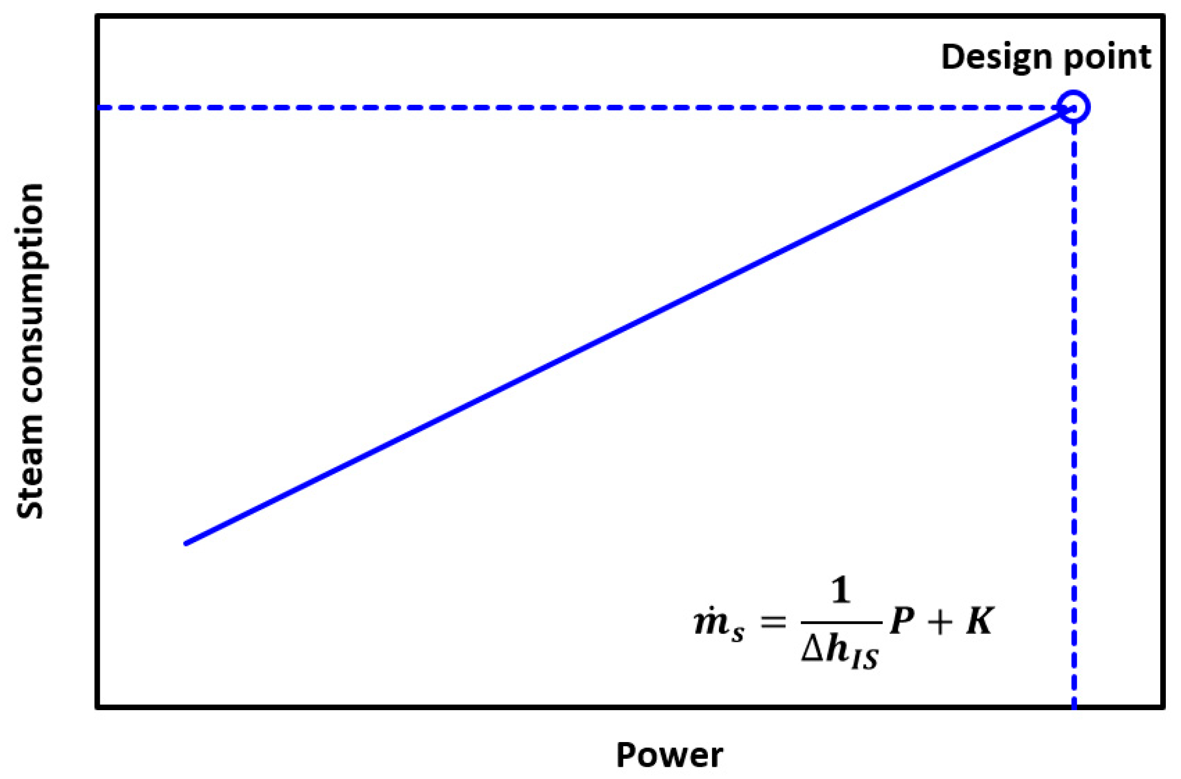
The optimal inner pipe diameter was used to calculate nominal performance parameters. For each case, respective assumptions were incorporated in the simulation program to obtain information on nominal HPS consumption. The isentropic enthalpy difference was then determined from the actual enthalpy difference calculated by the model, and the characteristics’ intercept was calculated directly, as seen in Equation (13):

$$K={\dot{m}}_S-\frac{1}{\Delta h_{IS}}P$$

(13)

For any point of the characteristics (different from the nominal point), isentropic efficiency can be calculated from Equation (14):

$${\eta }_{IS}=\frac{\Delta h}{\Delta h_{IS}}=\frac{\frac{W}{{\dot{m}}_S}}{\Delta h_{IS}}=\frac{\frac{\frac{P}{{\eta }_{mech}}}{\frac{1}{\Delta h_{IS}}P+K}}{\Delta h_{IS}}=\frac{P}{{\eta }_{mech}\left(P+\Delta h_{IS}K\right)}$$

(14)

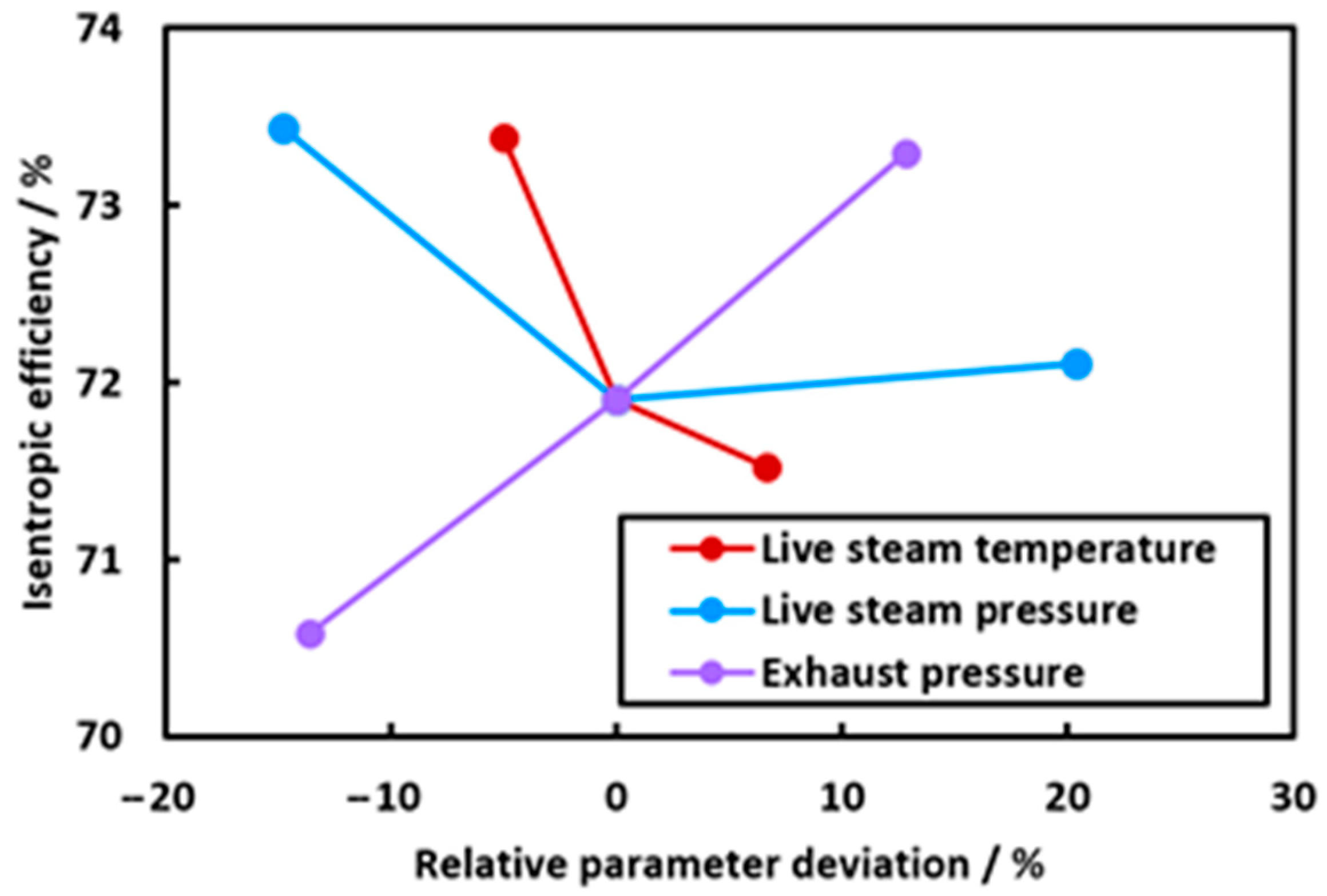
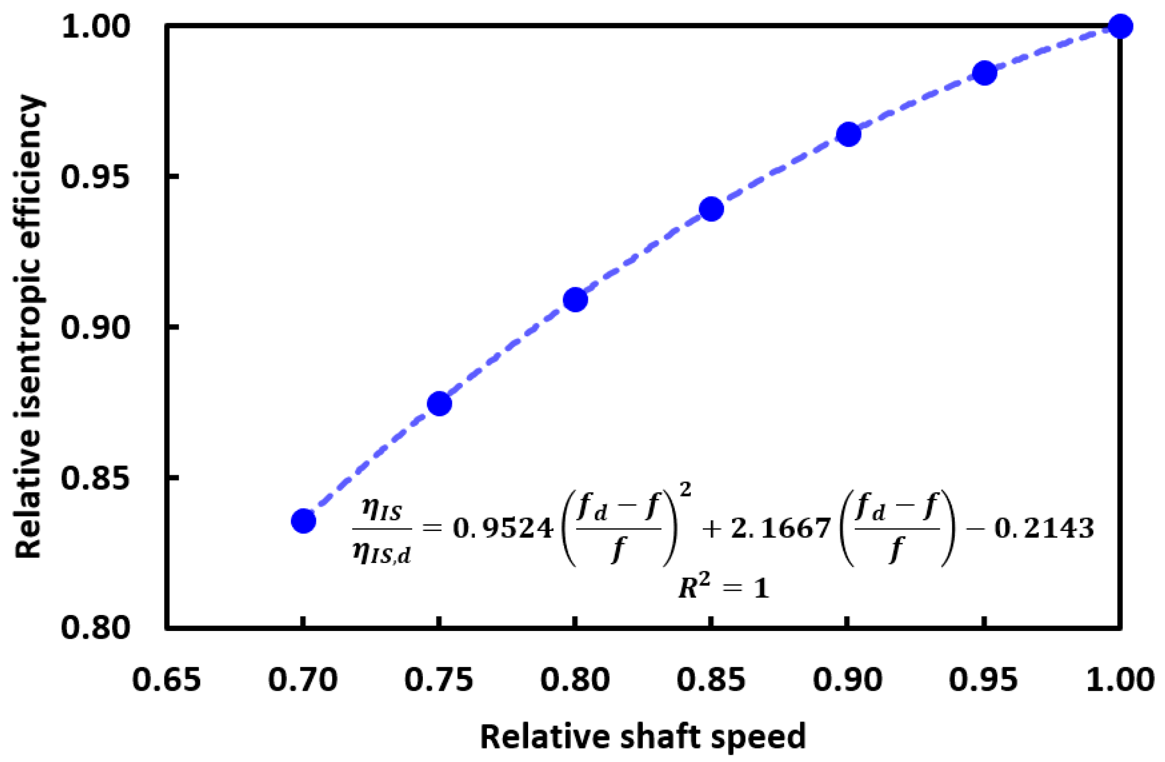
Polynomial fitting of the isentropic efficiencies provided parameters for Figure 19, which, as well as other characteristic parameters of the turbine, are summed up in

Table 4. Turbine characteristics.

	Ambient Temperature/°C	Nominal HPS Consumption/kg·h−1	Nominal Δh/kJ·kg−1	ΔhIS/kJ·kg−1	K/kg·s−1	a·107	b·104	c·102
Case 1	10	34,703	158.6	244.0	4.312	−2.101	7.169	6.953
	35	34,703	158.6	244.0	4.312	−2.101	7.169	6.953
	−14	34,724	158.5	243.8	4.314	−2.101	7.170	6.954
Case 2	10	34,685	158.8	244.3	4.314	−2.098	7.164	6.933
	35	34,682	158.8	244.3	4.313	−2.099	7.164	6.935
	−14	34,688	158.8	244.3	4.314	−2.098	7.163	6.930
Case 3	N/A	34,623	159.0	244.6	4.303	−2.100	7.168	6.947
Cases 4–6	N/A	33,954	162.1	249.4	4.219	−2.101	7.169	6.953
Case 7	10	42,782	128.7	198.0	5.318	−2.100	7.166	6.942
	35	42,707	128.9	198.3	5.308	−2.100	7.168	6.948
	−14	42,855	128.5	197.7	5.328	−2.103	7.178	6.953
Case 8	10	42,172	130.5	200.8	5.239	−2.101	7.170	6.955
	35	42,137	130.7	201.1	5.240	−2.098	7.159	6.945
	−14	42,208	130.4	200.6	5.244	−2.103	7.176	6.961
Case 9	N/A	41,182	133.7	205.7	5.119	−2.100	7.166	6.942

.

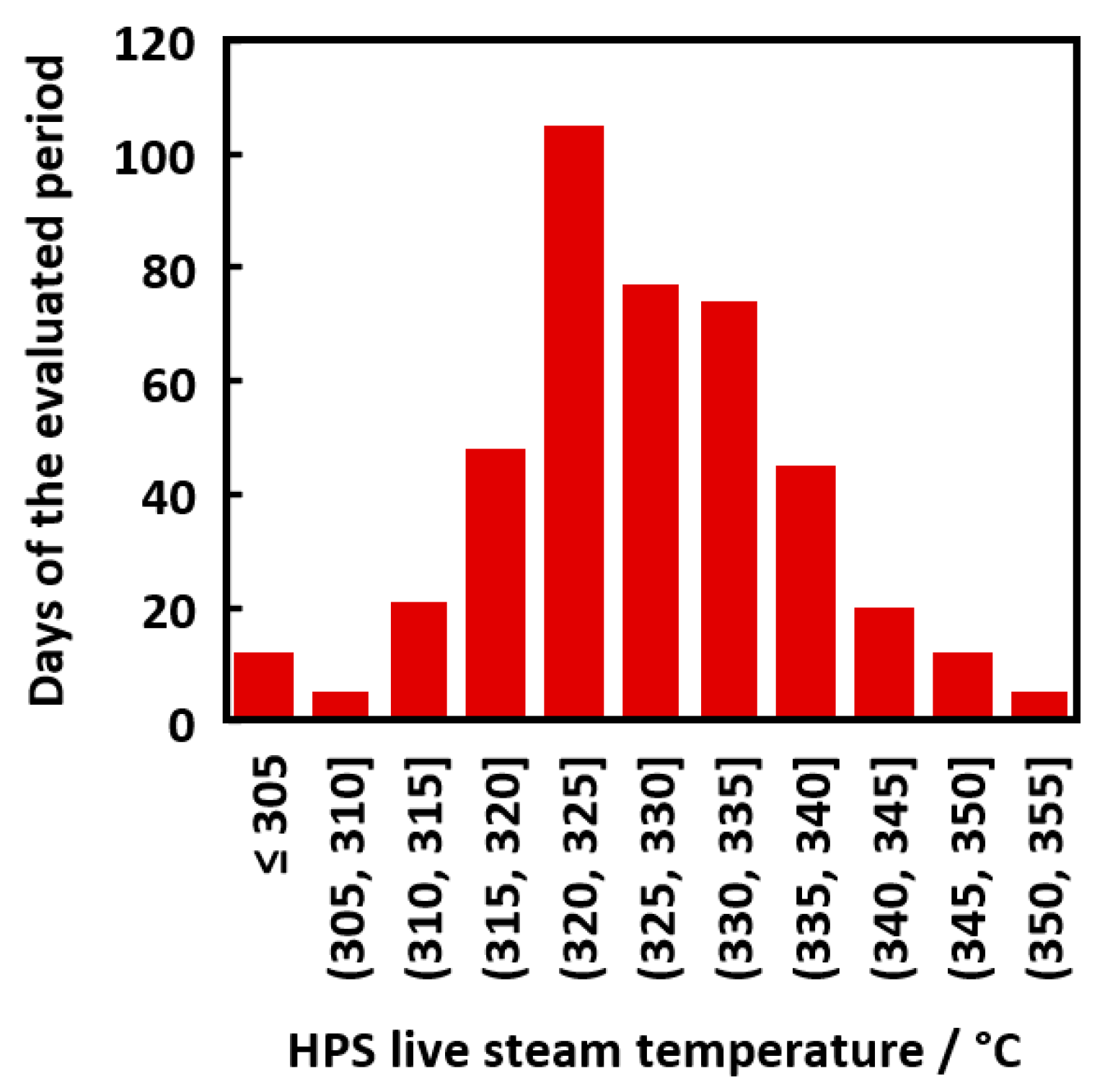
To account for ambient temperature variations during the evaluated period, discrete temperature peaks were considered. These encompassed the highest, the lowest, and the average ambient temperature measured in 2018. Because cases 4–6 did not consider the pipeline properties, turbine characteristics for these cases were identical as they shared the same design point.

As can be seen in Table 4, temperature fluctuations affected the steam consumption minimally. Due to high temperature of the transported medium (HPS, ~325 °C), the driving force of heat transfer depended only insignificantly on the change of ambient temperature. Thus, the ambient temperature variations could be neglected, and were not taken into further consideration.

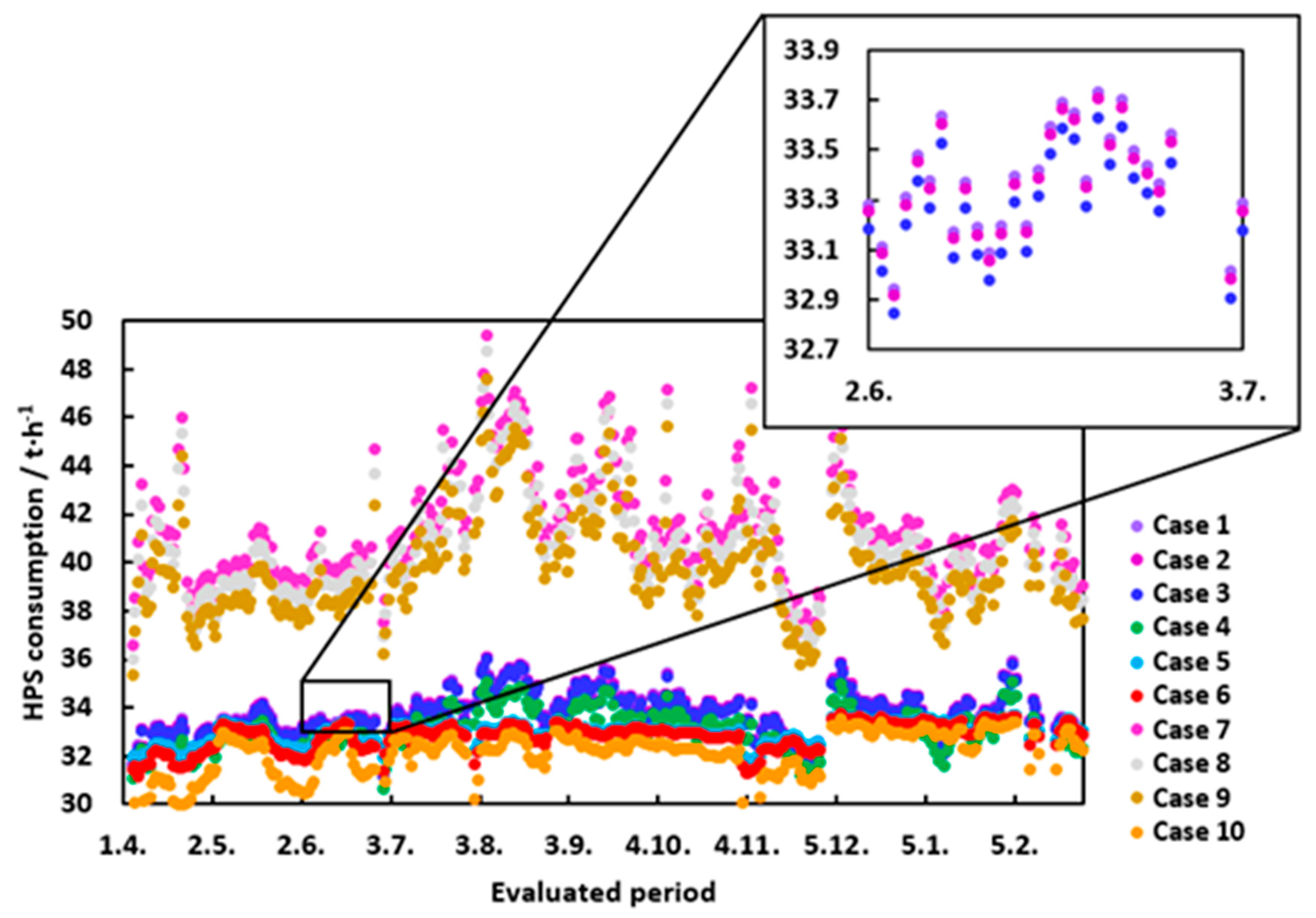
To visualize the differences between individual approaches, HPS consumption over the evaluated period using the methodology of each considered case was examined. For cases incorporating heat loss, the average ambient temperature (10 °C) was considered. In Figure 22, an evident discrepancy between the individual cases can be observed. Average deviations from the base cases (case 1 for actual pipeline length; case 7 for tenfold increase in pipeline length) are summarized in

Table 5. Comparison of different case results.

Base Case	Average Relative Deviation in HPS Consumption/%
	Case 2	Case 3	Case 4	Case 5	Case 6	Case 8	Case 9	Case 10
Case 1	0.08	0.31	2.21	2.32	2.84	-	-	5.01
Case 7	-	-	20.35	20.09	20.52	1.61	3.74	22.28

.

While the effect of heat losses from pipelines to the ambient space were proven to be minimal for the actual length of piping (average deviation ≤ 0.31%), a tenfold increase in the pipe length increased the average deviation up to 3.74%. Hence, heat loss increased linearly with the distance. An almost identical trend could be observed in the pressure drop calculation, however, with dramatically different impact on the calculated HPS consumption. Thus, for calculations comprising long pipelines, severe errors are to be expected if pressure drop is neglected. Furthermore, models not considering steam quality fluctuations (case 5) and compressor shaft speed variations (case 6) are not capable of predicting peaks in HPS consumption (provide different trends) and are thus unsuitable even for systems comprising short pipelines, though their average deviation is only slightly different to case 4.

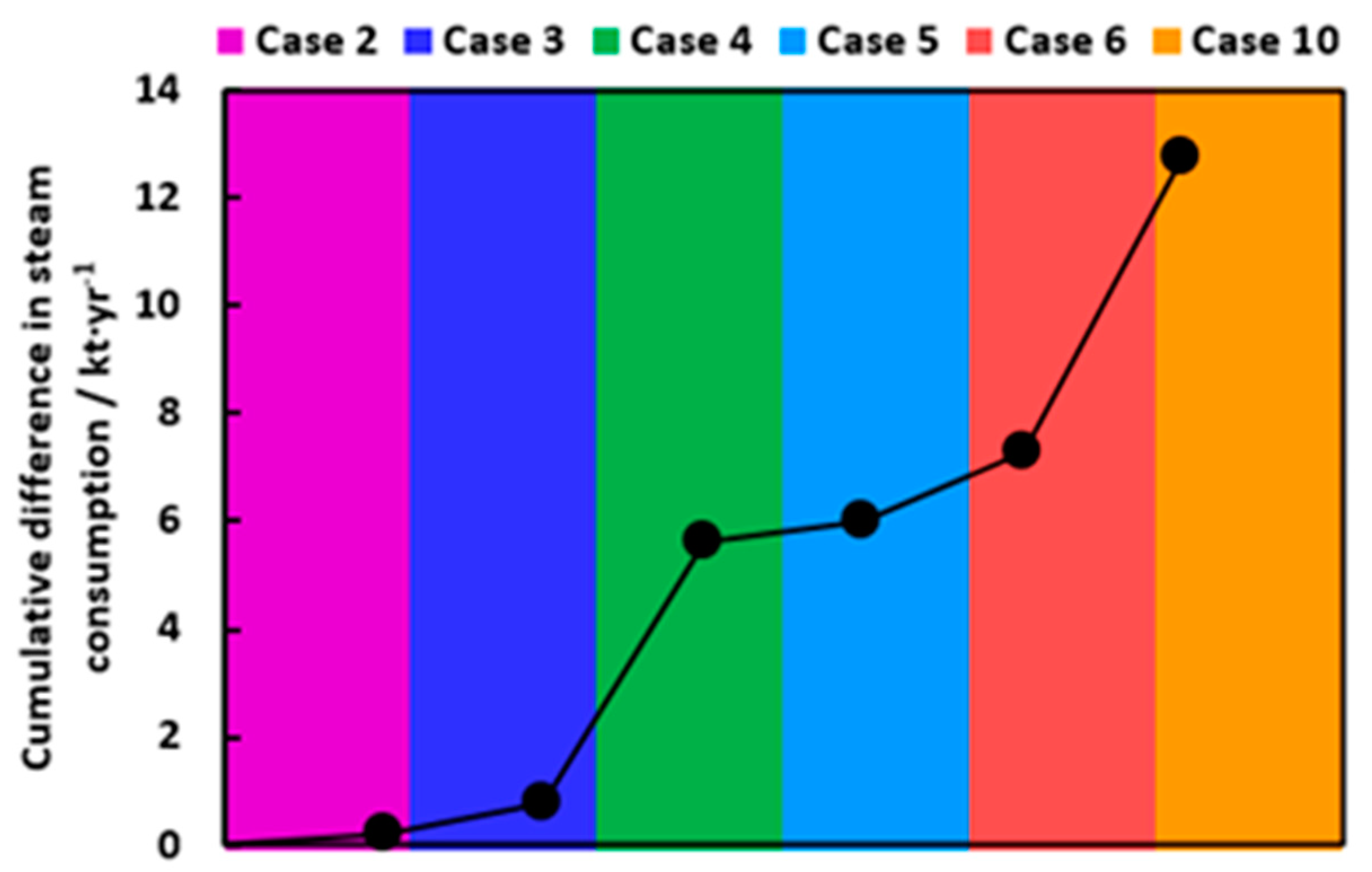
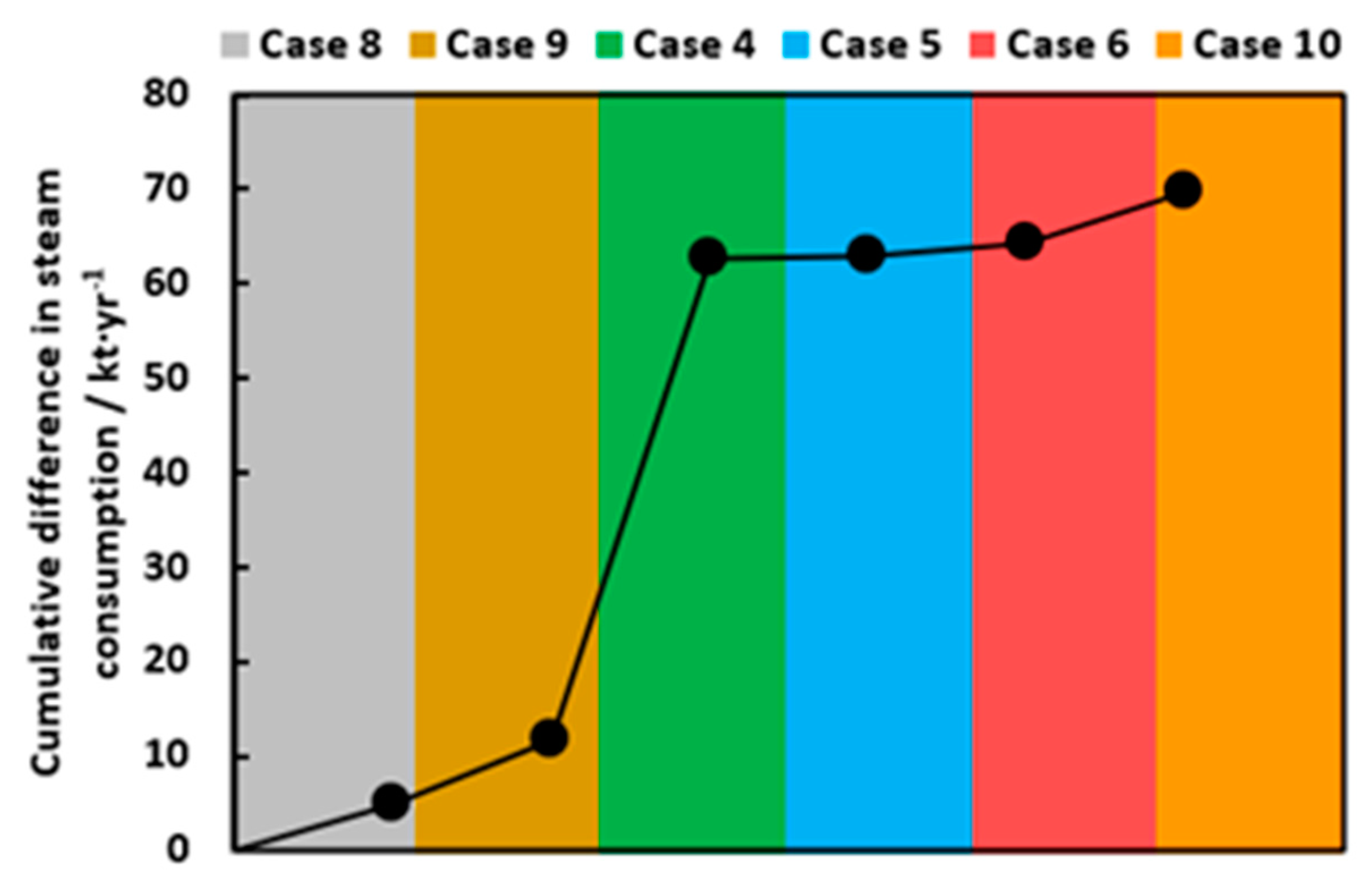
For a more comprehensive illustration, the yearly cumulative differences were displayed in Figure 23 and Figure 24 for case 1 and case 7, respectively. For the actual-size pipeline, two most significant contributions were visible: The first caused by neglecting the pipeline pressure drop and the second by considering a constant isentropic efficiency. The latter has proven to be the most severe, resulting in an almost 13 kt/y difference.

When considering a pipeline ten times the length of the actual pipeline, the effect of every simplification in the process drive sizing becomes more evident. However, in contrast to calculations of the actual pipeline, the pressure drop is the most crucial. Moreover, cumulative differences in HPS consumption prove the overall trend to be monotonic as opposed to average deviation of case 5 from case 7 (Table 5). These findings underline the fact that even though average deviations for some cases showed only slight differences, significant cumulative differences can occur. This, above all, affected the final economic evaluation.

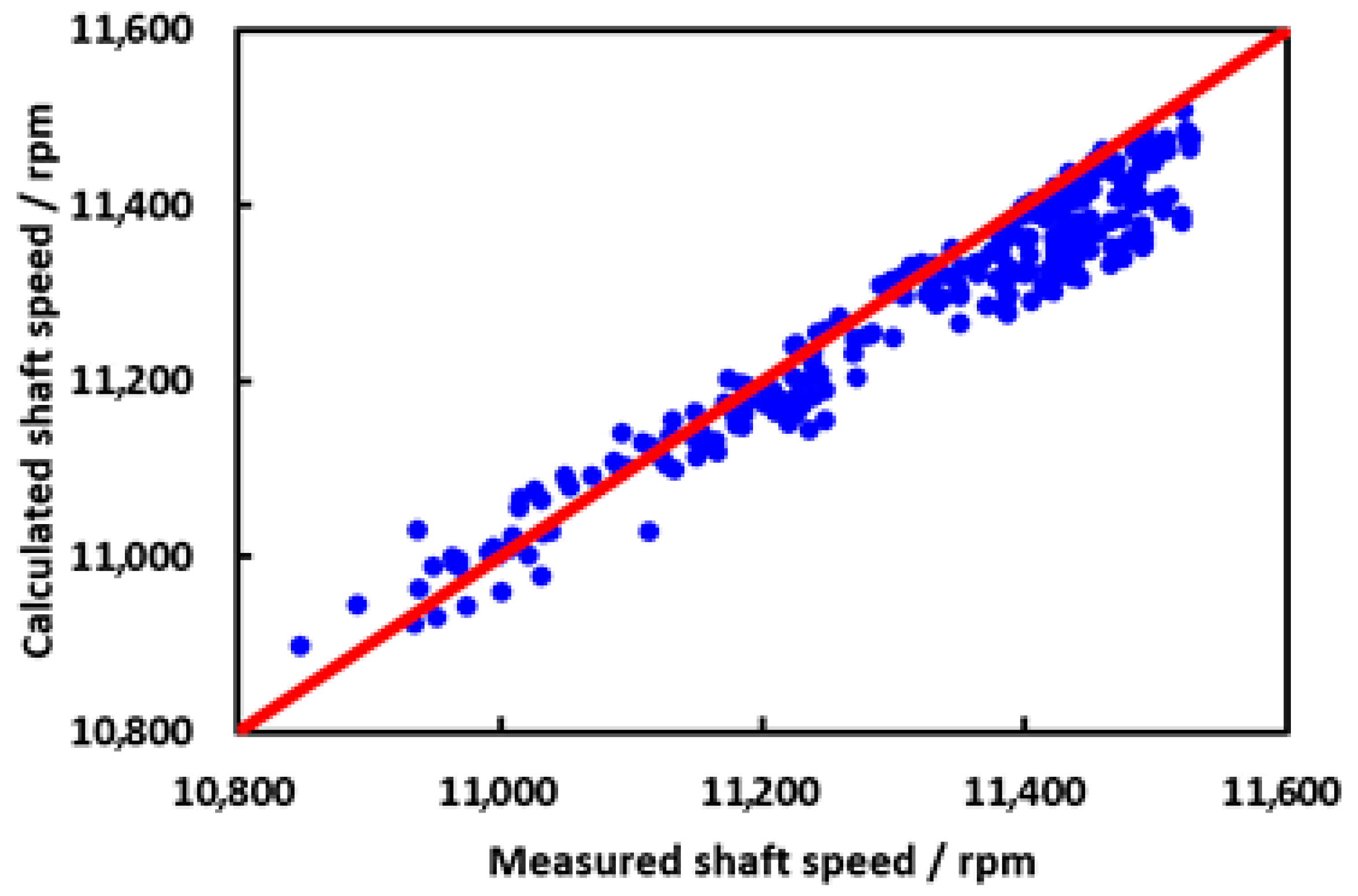
Practically every unit operates off-design for most of the operational time as the exact conditions defined as nominal are hardly ever met. However, the measure of deviation from the design parameters shows how well the equipment has been designed. To assess a possible negative impact of the steam drive replacement on the driven process, a study was conducted operating the turbine at full load for each case and each day of the evaluated period. The power output provided by the turbine consuming nominal amount of steam (Table 4) was compared to the actual power requirements of the process. A threshold of 5% (65 kW) was set, which is a typical design margin. In this study, again, results for the actual pipeline were compared to the ten-times-longer pipeline variant.

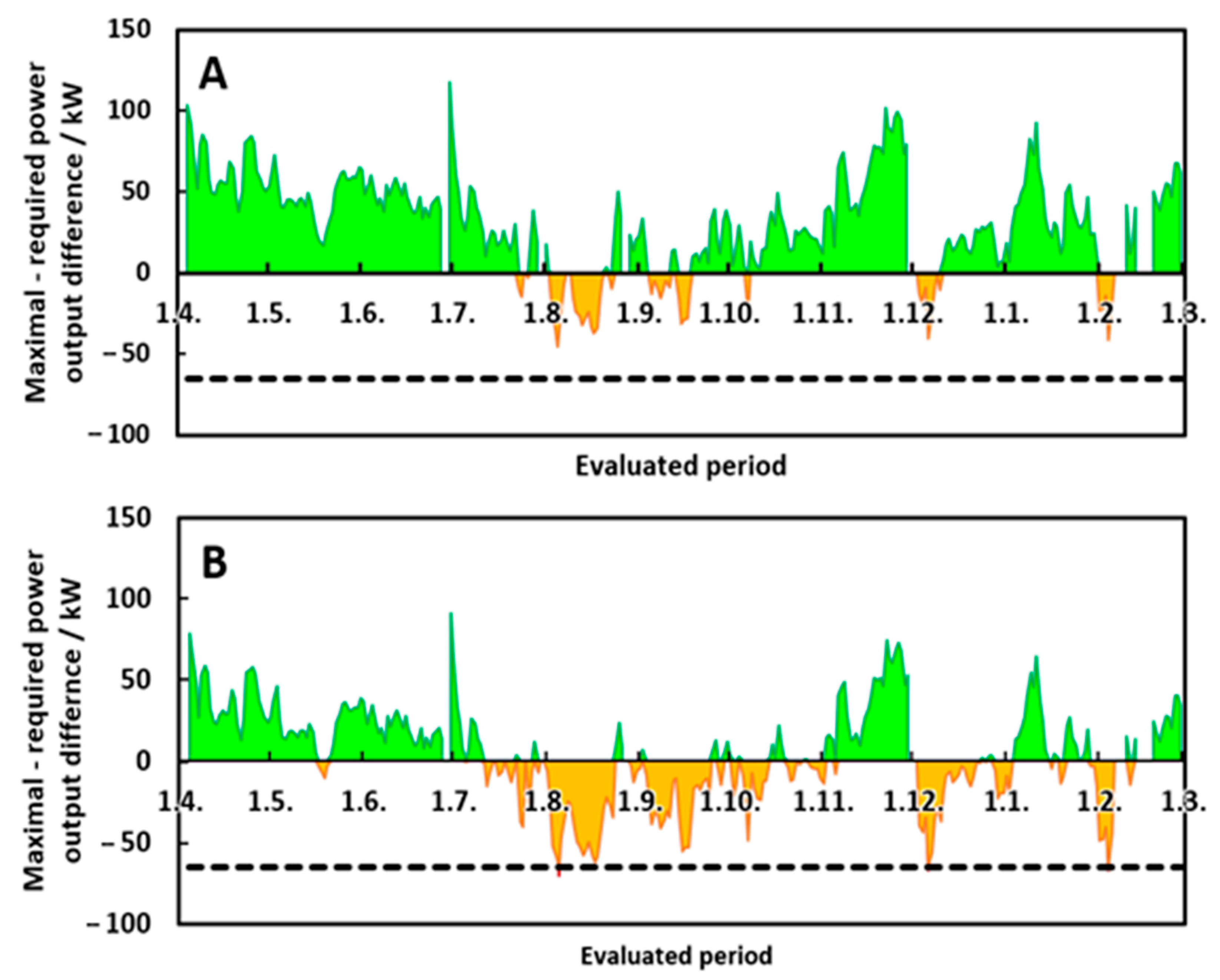
As shown in Figure 25, for a relatively short pipeline (≈100 m), a turbine designed with respect to all abovementioned aspects (Case 1) provided the process with the required power over the whole evaluated period. Simplified models, cases 4–6, also provided satisfactory results with hardly any threshold overshoots. However, the difference in the performance reserve was evident, pointing out nominal turbine inlet steam mass flow undersizing.

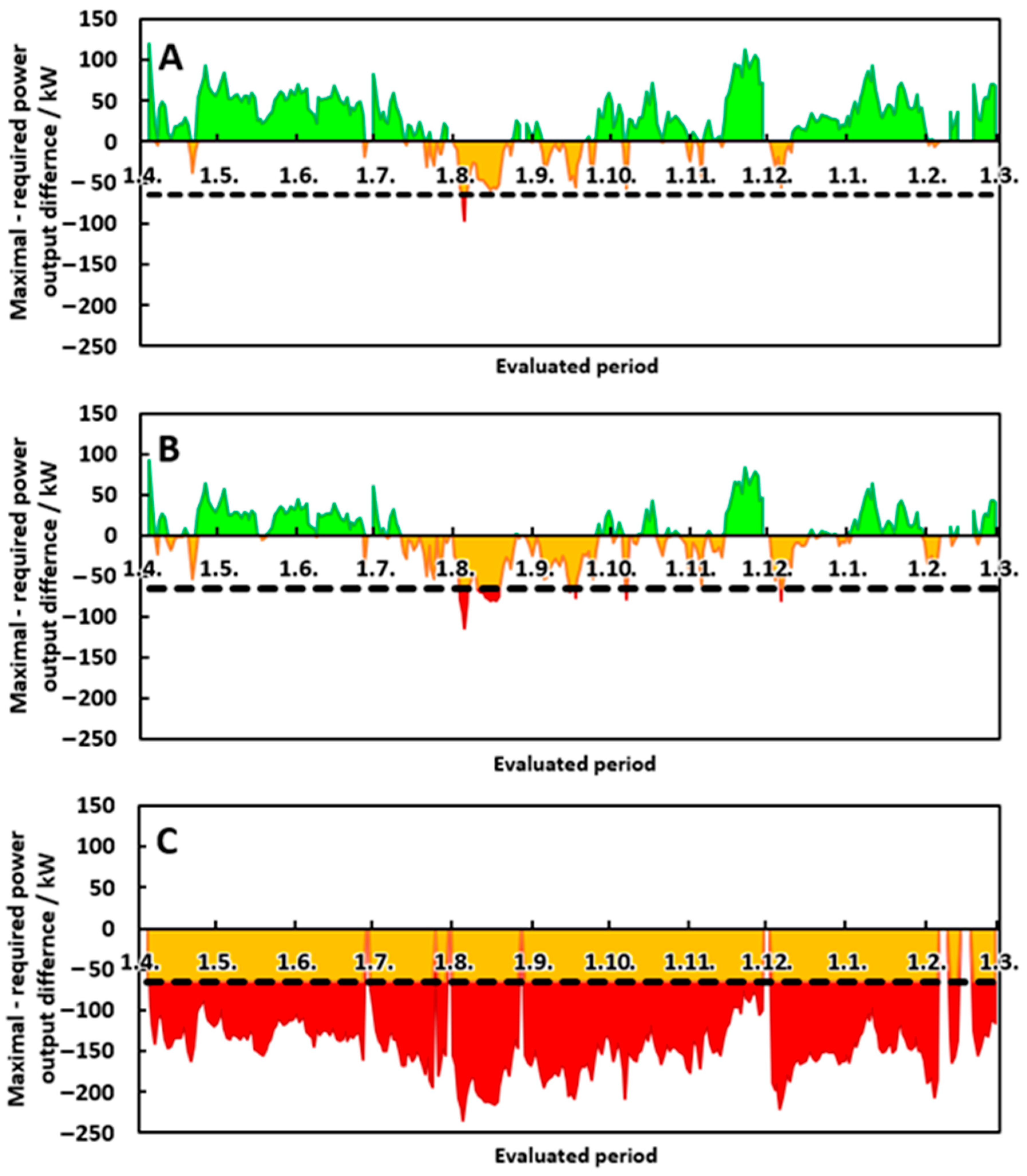
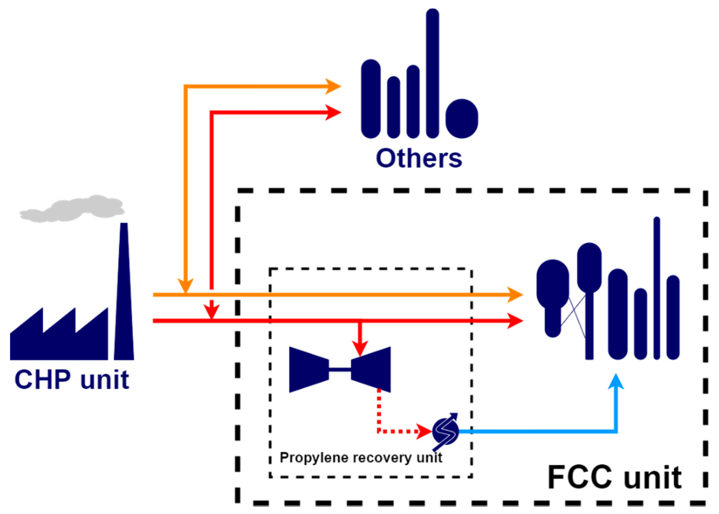
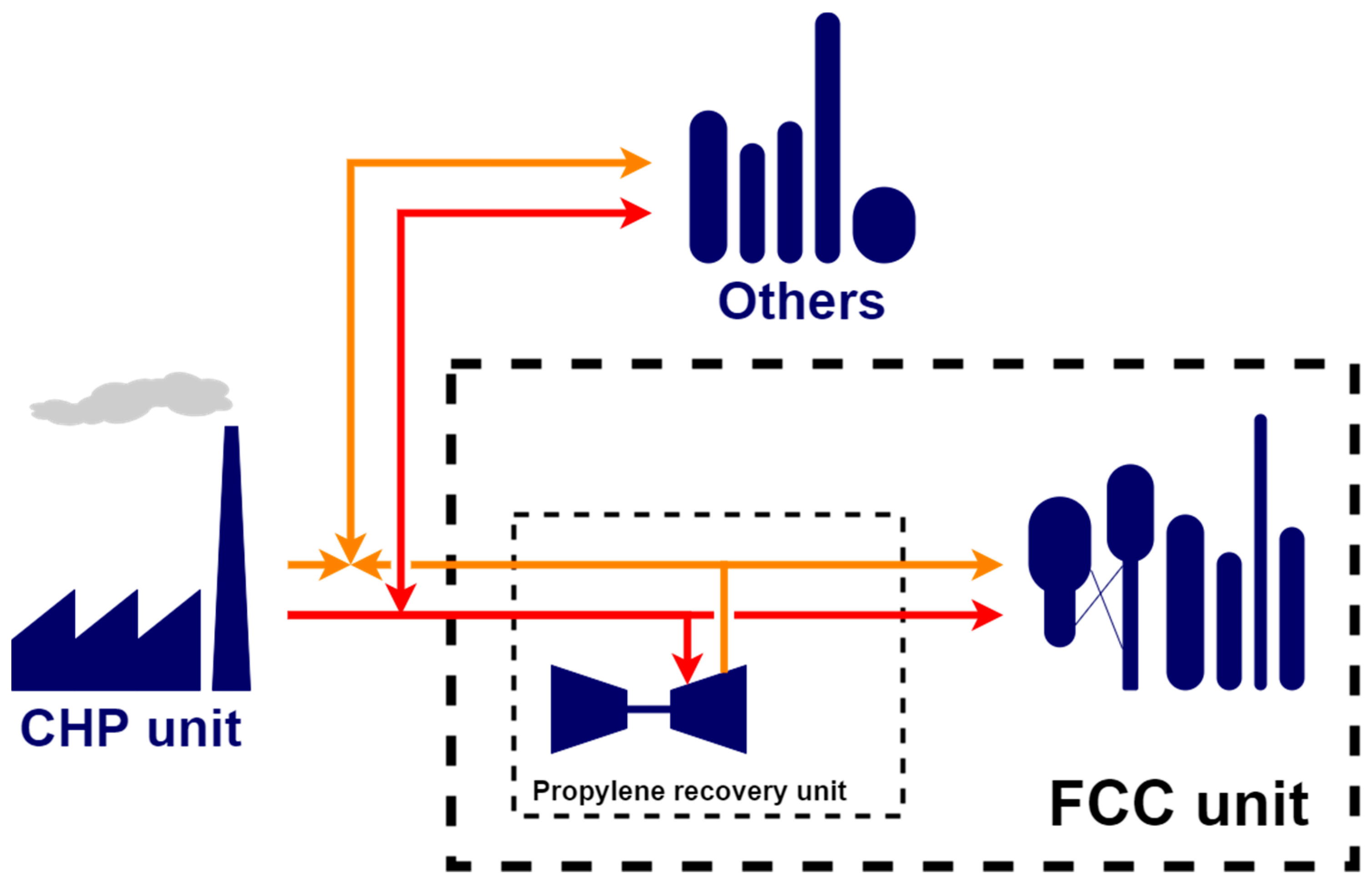
The situation changed dramatically with the increase in pipeline length. As depicted in Figure 26, even when all the aspects were considered (case 7), there was a short period of time when the turbine was not capable of providing the required mechanical power. The more such periods appeared, the less system properties were considered (e.g., case 9, which did not take heat loss into account). Finally, the worst-case scenario did not take pressure drop into account. As proven below, a turbine designed without regard to pressure drop along the pipeline did not provide the process with the required mechanical power with its lack exceeding 100 kW (approximately 8% of nominal mechanical power requirement) very frequently. The inability of the steam drive designed without steam frictional pressure losses consideration to meet the process-side mechanical power demand inevitably resulted in a decrease of processed C3 fraction mass flow. The C3 fraction splitting process could thus become a bottleneck of the whole FCC reaction products separation section with serious consequences on its profitability.

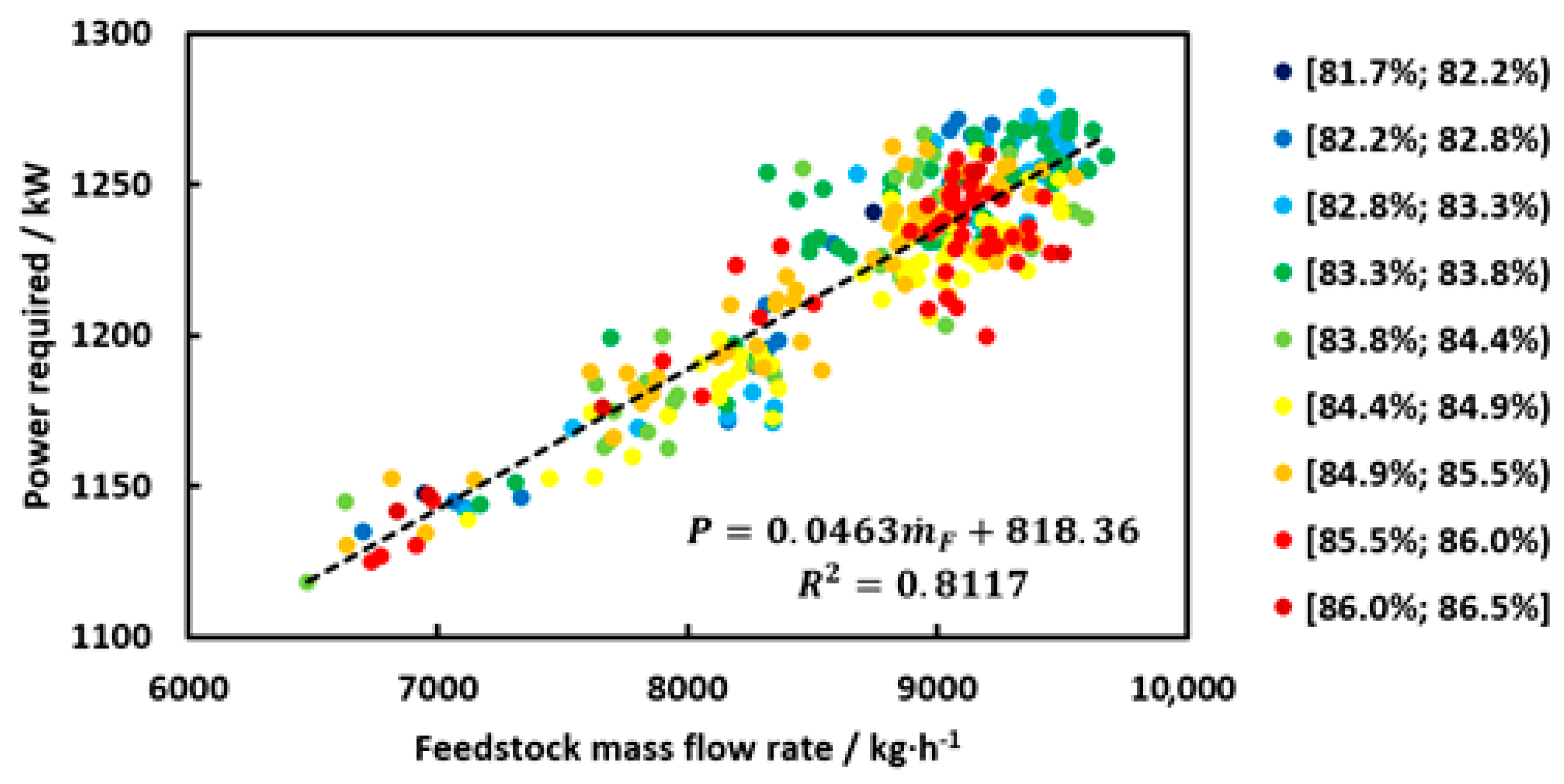
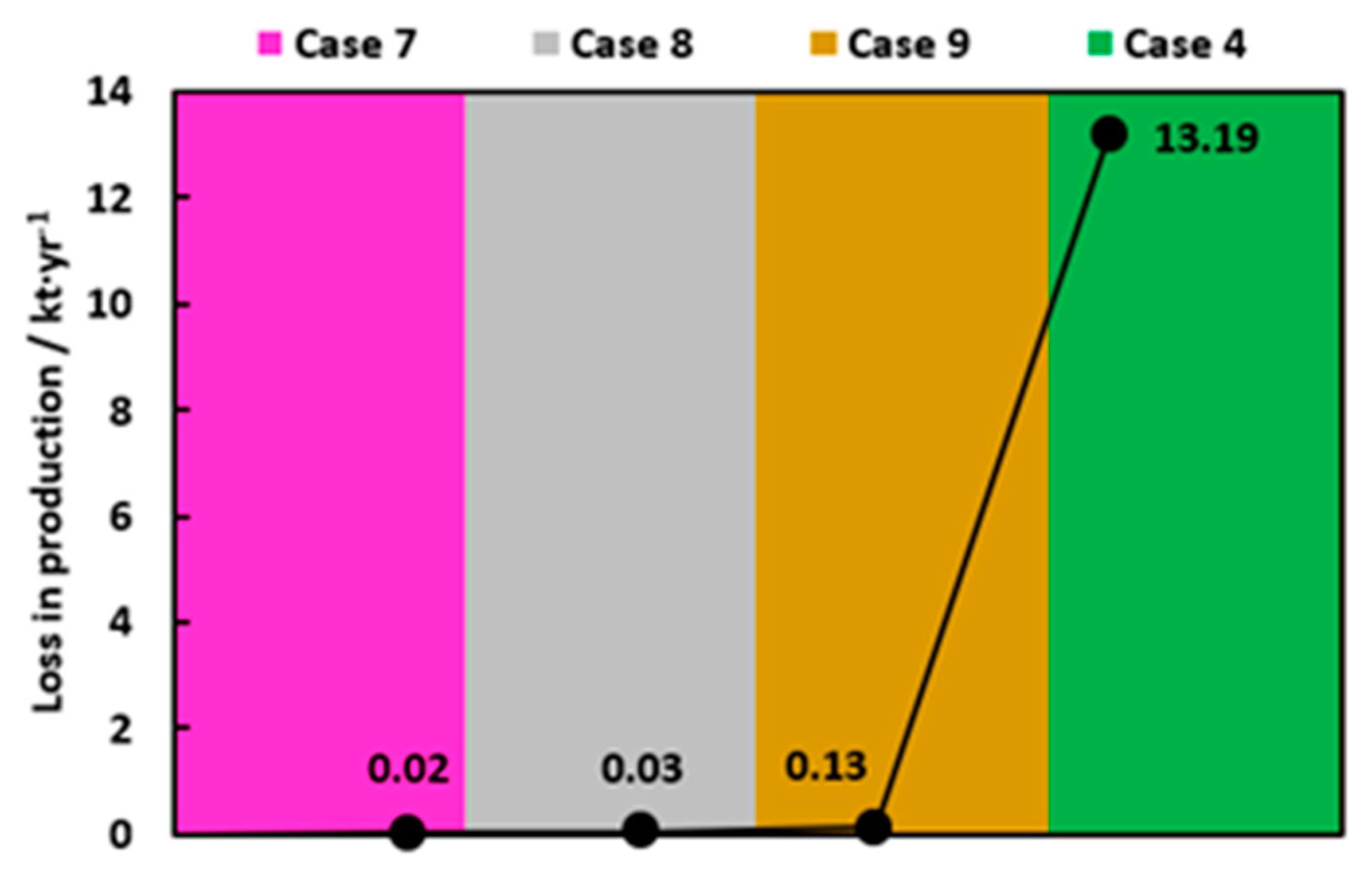
Based on the process side characteristics (Figure 10), production loss due to insufficient power supply can be quantified. Each 100 kW of lacking power output (i.e., power output below the dashed line in Figure 26) represented 2.16 t/h of production loss (Figure 27). For the studied propylene recovery unit processing approx. 65.8 kt of feedstock yearly, the decrease of 13.2 kt/y (20%) was unacceptable.

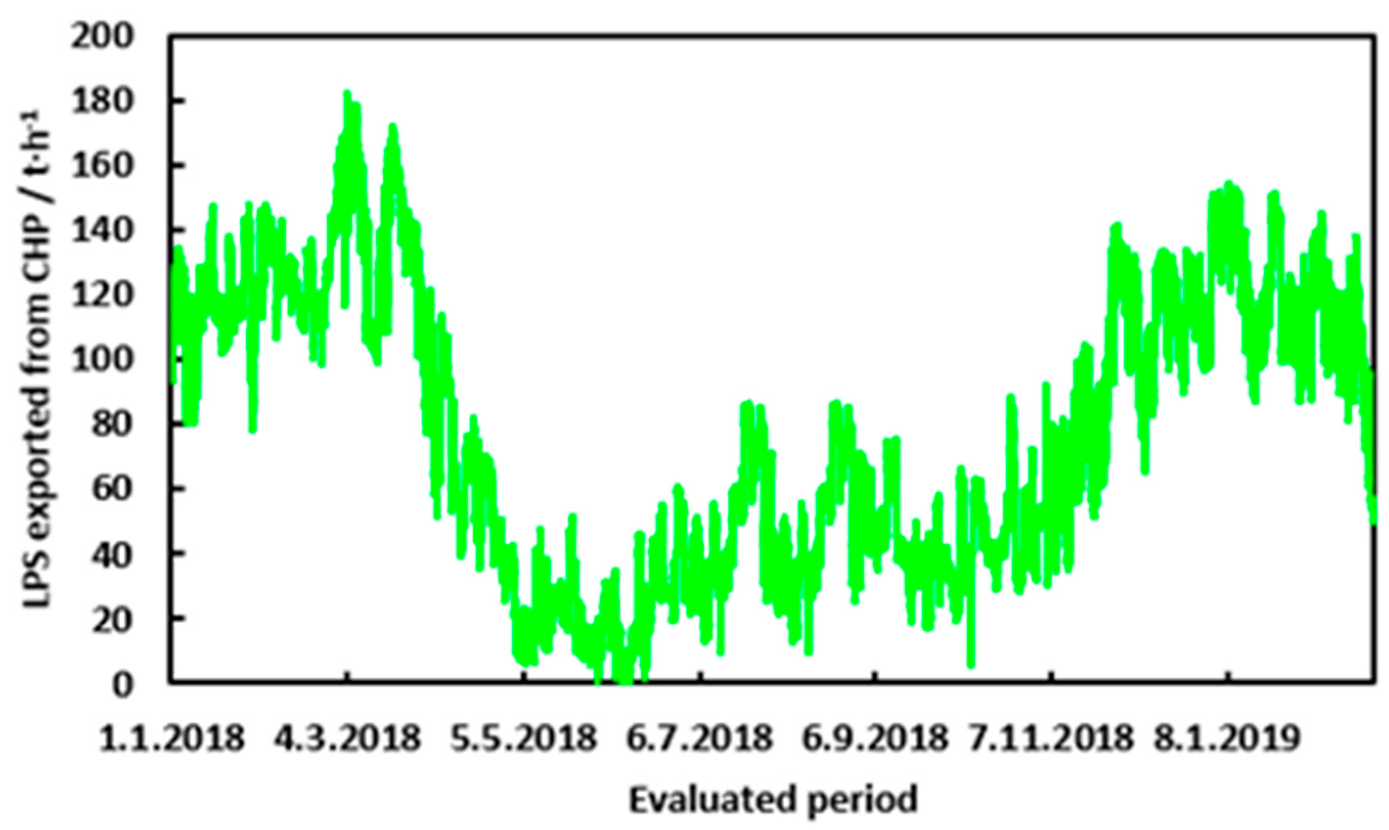
Besides the impact of the proposed steam drive change on the propylene recovery process, its effect on the operation of the refinery’s main HPS and MPS pipelines was assessed in terms of transported steam mass flow. A significant change in the steam mass flow may result in new bottlenecks or even an infeasible operation of the network [26]. Current HPS pipeline operation was analyzed in detail by Hanus et al. 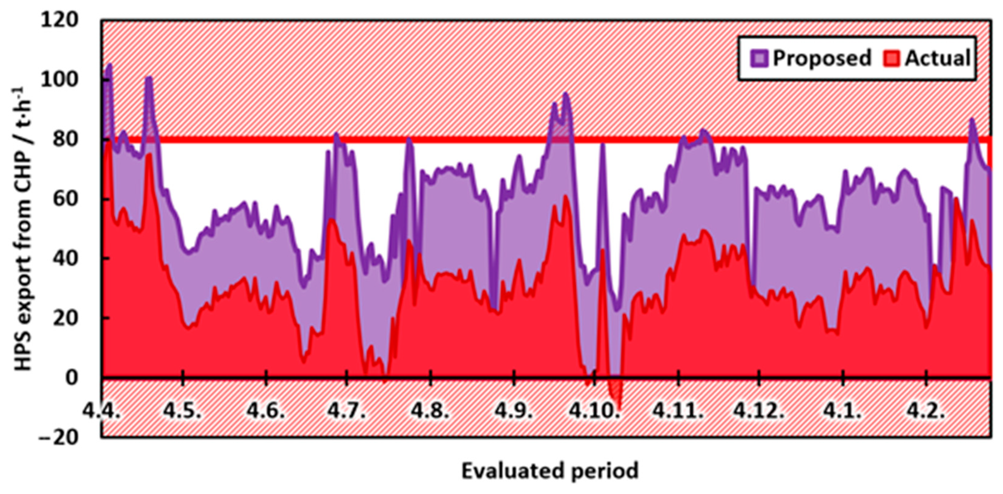[26], defining the safe operation window between 20 and 60 t/h of exported HPS from CHP. Such conditions prevent excessive erosion and pressure losses on one hand and steam stagnation in pipelines on the other. An existing pipeline, returning HPS to the CHP, enables HPS network operation with zero or even negative net HPS export from the CHP. Furthermore, exporting more than 60 t/h of HPS from the CHP is possible by utilizing a second main HPS pipeline that is normally closed but can be activated if needed. However, even with both the main HPS pipelines active, exporting more than 80 t/h HPS from the CHP for longer periods is unwanted, though possible. As shown in Figure 28, the proposed steam drive change eliminated the occurrence of undesirably low HPS export from the CHP and simultaneously led to HPS export of over 80 t/h in certain periods, forcing the steam network operators to undertake additional measures to ensure the HPS network stability.

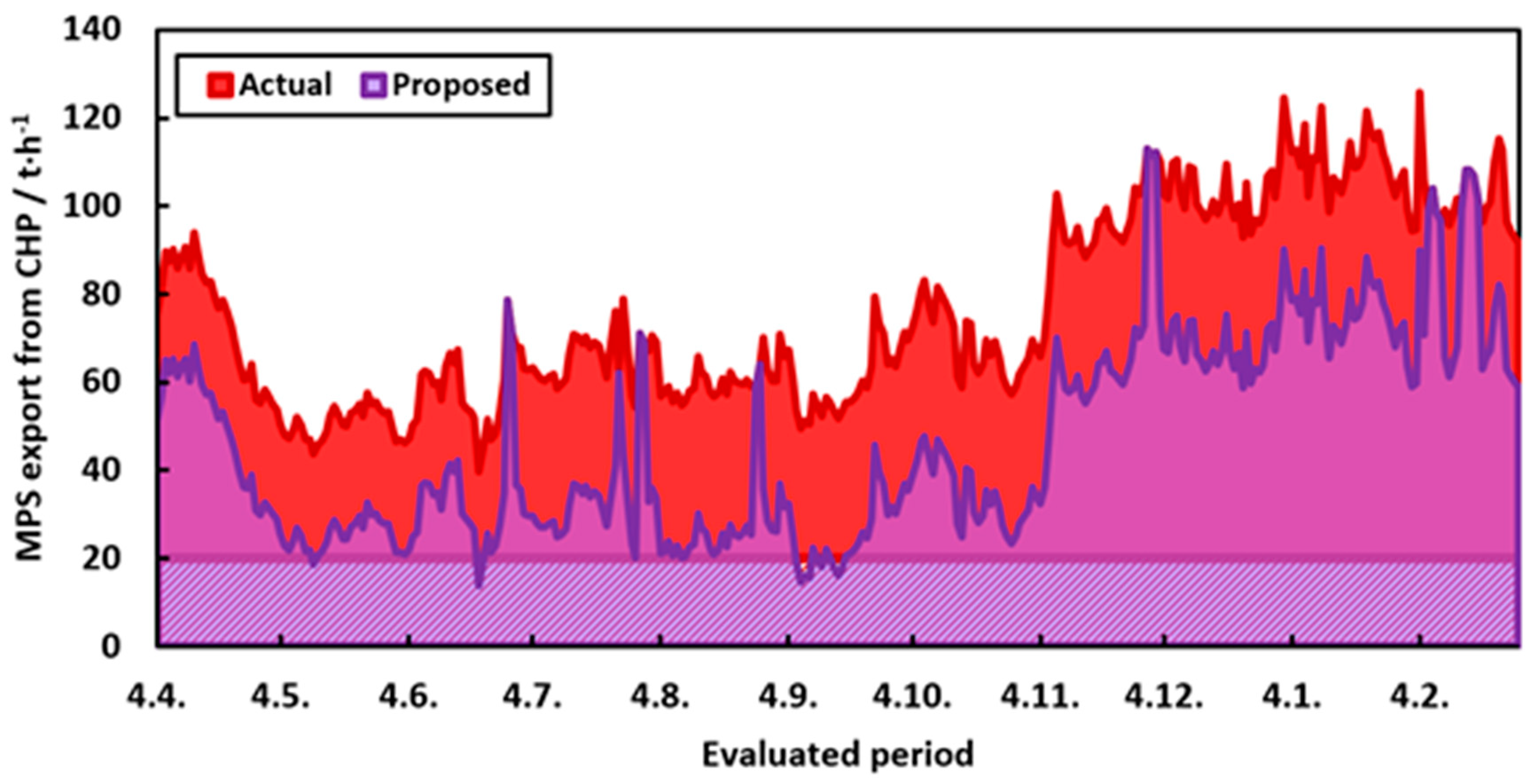
The MPS network operation was also investigated and the results are shown in Figure 29. Presently, the MPS demand of the refinery exceeds 80 or even 100 t/h, which strains the MPS production capacity of the CHP. MPS export of over 100 t/h cannot usually be met by steam extraction and the deficit has to be covered by 9 MPa steam throttling in the CHP. As presented in Figure 29, the occurrence of such unwanted states is strongly reduced by the new process drive in operation. A few periods appear, though, with MPS export below 20 t/h, which may affect the MPS network operation stability and have to be avoided by active MPS network management.

The change in exported steam mass flow at high-pressure and middle-pressure levels affects fuel consumption and carbon dioxide emissions of the CHP. The resulting effect differs according to the season of the year:

• In colder months (October to April), fuel is saved, and CO₂ emissions are reduced. Backpressure power production in the CHP is also reduced;
• In warmer months (May to September), the reduction in the CHP backpressure power production is compensated by an increase in the condensing production which keeps the total power output of the CHP unchanged. The resulting change in fuel consumption and in CO₂ emissions production is determined by the difference between: (a) Marginal condensing power production efficiency of the CHP and, (b) the condensing mechanical power production in the replaced condensing steam drive.

Based on discussion with CHP managers and operators, the following input data were considered in calculations:

• Average thermal efficiency of the CHP is 85%, determined as the ratio of the enthalpy in exported steam to the fuel lower heating value;
• Heavy fuel oil combusted in the CHP produces 3.2 tons of CO₂ per 1 ton of oil;
• Marginal efficiency of the condensing power production in the CHP is 3 MWh per ton of combusted fuel.

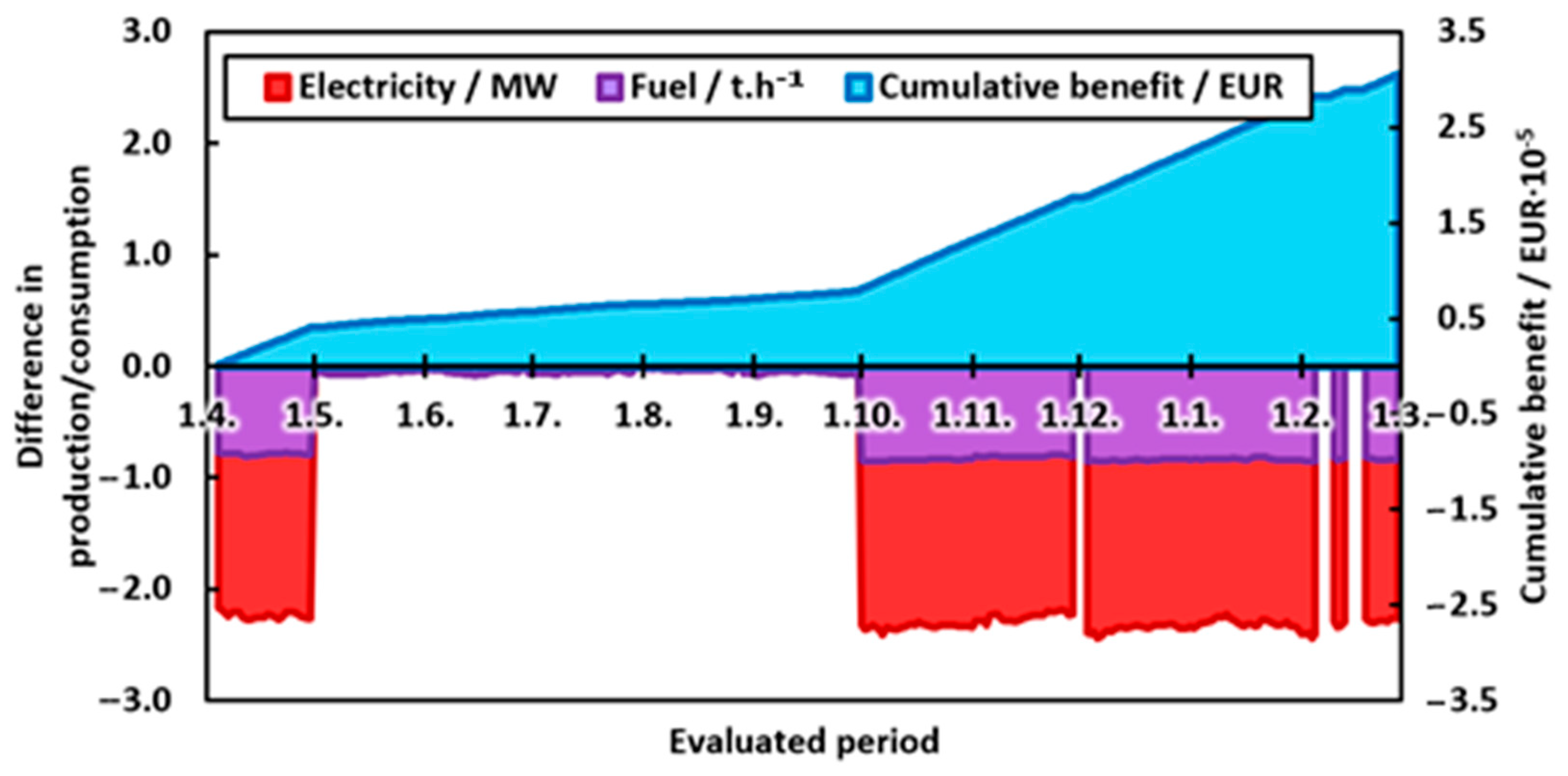
Trends of fuel consumption change and CHP electric power output decrease in the evaluated period are visualized in Figure 30.

Evaluation of the economic potential of the condensing steam drive replacement assumed the following prices: Electricity 45 €/MWh; heavy fuel oil 120 €/t; and CO₂ emissions 27 €/t. The hourly benefit results from (1) the achieved decrease in fuel consumption and in CO₂ emissions, and (2) the amount of additional power purchased from the outer grid. Additional power has to be purchased to balance the lower CHP output in colder months (Figure 30). The cumulative benefit curve (Figure 30) is obtained by summing up the hourly benefits over the evaluated period. As can be seen, most of the benefit is harvested during colder months. Overall, 3.72 kt/year of fuel can be saved and CO₂ emissions from the CHP can be reduced by 11.13 kt/year as a result of the process steam drive replacement. The resulting benefit is expected to be over 300,000 EUR/year. A preliminary estimate of the steam drive replacement cost including new pipelines is around 450,000 EUR, leading to a preliminary simple payback period of 1.5 years. Due to the envisioned CO₂ emission cost increase, economic feasibility of this proposal should be retained even if the fuel price decreases or that of purchased electricity increases.

Considering the results presented in Figure 25, it can be concluded that the C3 fraction feed processing capacity is met even with less rigorous steam drive sizing method. However, for the alternative with ten-times-longer pipelines, only the rigorous method presented in this paper ensures the retained process throughput capacity. Less complex sizing methods led to undersizing of the steam drive and the resulting processing capacity limitation (see Figure 27) outweighed the economic potential of the steam drive replacement (Figure 30) by far.

The presented technical and economic results varied significantly depending on the type and operation of the CHP that served as a marginal steam source. Modern industrial CHP units usually comprise a gas turbine-based combined cycle. If such a unit operates in a purely cogeneration mode (no or minimal condensing power production), the resulting change in fuel consumption and power production is different from that in Figure 30. Apart from the electricity production change due to the steam balance shift on HPS and MPS levels, either (a) an increase in condensing power production due to utilization of the saved HPS, or, (b) a decrease in the power output of gas turbine(s) and the associated fuel consumption reduction can be observed. The way is chosen by the CHP managers based on fuel costs compared to marginal power production cost in the combined cycle. In any case, since the combined cycle is a more efficient marginal cogeneration steam source than a traditional steam CHP, the resulting fuel consumption and CO₂ emissions release is lower. This further accentuates the need to analyze the marginal steam source operation carefully prior to steam drive sizing.

5. Conclusions

The presented method for process steam drive sizing comprises both process and steam network including the marginal steam source operation assessment. A proper investigation of both process-side and steam-side design and operation parameters is necessary and should precede the drive sizing itself. Attention should be paid to key process parameters including the required power input and its hourly and seasonal variability as well as the variability of the driven equipment frequency. Driving steam quality and discharge steam pressure variations should be evaluated carefully, and their change due to frictional pressure and heat losses from steam pipelines should also be assessed. Driving and discharge steam pressure levels should be chosen according to the analysis of individual steam pressure levels’ operation range and their anticipated change resulting from steam drive implementation. Their effect on the marginal steam source operation should be evaluated considering all previous findings.

The proposed method comprises process data evaluation and calculations in a linked MATLAB^® and Aspen Plus^® environment. Thereby, the potential of MATLAB in process data analysis and results evaluation and visualization is coupled with the ability of rigorous process simulation by Aspen Plus^®.

The industrial case study comprised the replacement of the existing condensing steam drive by a new backpressure one, driving the 1.25 MW compressor of the heat pump-assisted C3 fraction splitting process. Application of the proposed method and comparison with the results obtained using methods proposed by other authors revealed that:

• Steam drive undersizing resulted from lower complexity of the sizing methods;
• Neglecting the variable frequency of the driven equipment, frictional pressure losses, and the steam drive efficiency loss at partial load operation could decrease the ability of the steam drive to provide the power required for the process;
• The simplest sizing method combined with the ten-times-longer steam pipeline led to a C3 fraction splitting capacity decrease of around 20%, which was unacceptable.

Examination of the changes in the HPS and MPS network operation revealed that several capacity bottlenecks could be removed by the steam drive replacement, but new ones could arise, which requires active steam network management. The impact on the CHP operation included fuel savings of up to 3.72 kt/year, and a CO₂ emissions reduction of 11.13 kt/year at the expense of an additional 17.29 GWh/year of power purchased from outer grid compensating for the power production decrease at the CHP. Warmer months’ contribution to this cost was negligible as the CHP compensated for the lowered backpressure power production by the expensive condensing one. Despite this fact, the proposed steam drive replacement exhibited a simple payback period shorter than two years.

Further method improvement will be aimed in future work with the focus on implementing multi-objective optimization. The effects of steam drive implementation or replacement of the main steam network operation should be examined and assessed more closely.

References

1. Murugan, S.; Horák, B. Tri and polygeneration systems—A review. Renew. Sustain. Energy Rev. 2016, 60, 1032–1051. [Google Scholar] [CrossRef]
2. Jana, K.; Ray, A.; Majoumerd, M.M.; Assadi, M.; De, S. Polygeneration as a future sustainable energy solution—A comprehensive review. Appl. Energy 2017, 202, 88–111. [Google Scholar] [CrossRef]
3. Baláž, V.; Nežinský, E.; Jeck, T.; Filčák, R. Energy and Emission Efficiency of the Slovak Regions. Sustainability 2020, 12, 2611. [Google Scholar] [CrossRef] [Green Version]
4. Brożyna, J.; Strielkowski, W.; Fomina, A.; Nikitina, N. Renewable Energy and EU 2020 Target for Energy Efficiency in the Czech Republic and Slovakia. Energies 2020, 13, 965. [Google Scholar] [CrossRef] [Green Version]
5. Rehfeldt, M.; Worrell, E.; Eichhammer, W.; Fleiter, T. A review of the emission reduction potential of fuel switch towards biomass and electricity in European basic materials industry until 2030. Renew. Sustain. Energy Rev. 2020, 120, 109672. [Google Scholar] [CrossRef]
6. Korkmaz, P.; Gardumi, F.; Avgerinopoulos, G.; Blesl, M.; Fahl, U. A comparison of three transformation pathways towards a sustainable European society—An integrated analysis from an energy system perspective. Energy Strategy Rev. 2020, 28, 100461. [Google Scholar] [CrossRef]
7. Martins, F.; Felgueiras, C.; Smitkova, M.; Caetano, N. Analysis of Fossil Fuel Energy Consumption and Environmental Impacts in European Countries. Energies 2019, 12, 964. [Google Scholar] [CrossRef] [Green Version]
8. Malinauskaite, J.; Jouhara, H.; Ahmad, L.; Milani, M.; Montorsi, L.; Venturelli, M. Energy efficiency in industry: EU and national policies in Italy and the UK. Energy 2019, 172, 255–269. [Google Scholar] [CrossRef]
9. Linares, P.; Pintos, P.; Würzburg, K. Assessing the potential and costs of reducing energy demand. Energy Transit. 2017, 1, 4. [Google Scholar] [CrossRef] [Green Version]
10. Maciková, L.; Smorada, M.; Dorčák, P.; Beug, B.; Markovič, P. Financial Aspects of Sustainability: An Evidence from Slovak Companies. Sustainability 2018, 10, 2274. [Google Scholar] [CrossRef] [Green Version]
11. Lieskovský, M.; Trenčiansky, M.; Majlingová, A.; Jankovský, J. Energy Resources, Load Coverage of the Electricity System and Environmental Consequences of the Energy Sources Operation in the Slovak Republic—An Overview. Energies 2019, 12, 1701. [Google Scholar] [CrossRef] [Green Version]
12. Ghoniem, A.F. Needs, resources and climate change: Clean and efficient conversion technologies. Prog. Energy Combust. Sci. 2011, 37, 15–51. [Google Scholar] [CrossRef]
13. Sutherland, B.R. Sustainably Heating Heavy Industry. Joule 2020, 4, 14–16. [Google Scholar] [CrossRef]
14. Rivas, D.F.; Castro-Hernández, E.; Villanueva Perales, A.L.; van der Meer, W. Evaluation method for process intensification alternatives. Chem. Eng. Process.-Process Intensif. 2018, 123, 221–232. [Google Scholar] [CrossRef]
15. Ifaei, P.; Safder, U.; Yoo, C. Multi-scale smart management of integrated energy systems, Part 1: Energy, economic, environmental, exergy, risk (4ER) and water-exergy nexus analyses. Energy Convers. Manag. 2019, 197, 111851. [Google Scholar] [CrossRef]
16. Safder, U.; Ifaei, P.; Yoo, C. Multi-scale smart management of integrated energy systems, Part 2: Weighted multi-objective optimization, multi-criteria decision making, and multi-scale management (3M) methodology. Energy Convers. Manag. 2019, 198, 111830. [Google Scholar] [CrossRef]
17. Rong, A.; Lahdelma, R. Role of polygeneration in sustainable energy system development challenges and opportunities from optimization viewpoints. Renew. Sustain. Energy Rev. 2016, 53, 363–372. [Google Scholar] [CrossRef] [Green Version]
18. Pintarič, Z.N.; Varbanov, P.S.; Klemeš, J.J.; Kravanja, Z. Multi-objective multi-period synthesis of energy efficient processes under variable environmental taxes. Energy 2019, 189, 116182. [Google Scholar] [CrossRef]
19. Al Moussawi, H.; Fardoun, F.; Louahlia, H. Selection based on differences between cogeneration and trigeneration in various prime mover technologies. Renew. Sustain. Energy Rev. 2017, 74, 491–511. [Google Scholar] [CrossRef]
20. Bamufleh, H.S.; Ponce-Ortega, J.M.; El-Halwagi, M.M. Multi-objective optimization of process cogeneration systems with economic, environmental, and social tradeoffs. Clean Technol. Environ. Policy 2012, 15, 185–197. [Google Scholar] [CrossRef]
21. Chen, Z.; Wang, J. Heat, mass, and work exchange networks. Front. Chem. Sci. Eng. 2012, 6, 484–502. [Google Scholar] [CrossRef]
22. Chew, K.; Klemeš, J.; Alwi, S.; Manan, Z.; Reverberi, A. Total Site Heat Integration Considering Pressure Drops. Energies 2015, 8, 1114–1137. [Google Scholar] [CrossRef] [Green Version]
23. Fan, Y.V.; Chin, H.H.; Klemeš, J.J.; Varbanov, P.S.; Liu, X. Optimisation and process design tools for cleaner production. J. Clean. Prod. 2020, 247, 119181. [Google Scholar] [CrossRef]
24. Frate, G.F.; Ferrari, L.; Lensi, R.; Desideri, U. Steam expander as a throttling valve replacement in industrial plants: A techno-economic feasibility analysis. Appl. Energy 2019, 238, 11–21. [Google Scholar] [CrossRef]
25. Ge, Z.; Zhang, F.; Sun, S.; He, J.; Du, X. Energy Analysis of Cascade Heating with High Back-Pressure Large-Scale Steam Turbine. Energies 2018, 11, 119. [Google Scholar] [CrossRef] [Green Version]
26. Hanus, K.; Variny, M.; Illés, P. Assessment and Prediction of Complex Industrial Steam Network Operation by Combined Thermo-Hydrodynamic Modeling. Processes 2020, 8, 622. [Google Scholar] [CrossRef]
27. Kler, A.M.; Stepanova, E.L.; Maksimov, A.S. Investigating the efficiency of a steam-turbine heating plant with a back-pressure steam turbine and waste-heat recovery. Thermophys. Aeromech. 2019, 25, 929–938. [Google Scholar] [CrossRef]
28. Liew, P.Y.; Wan Alwi, S.R.; Varbanov, P.S.; Manan, Z.A.; Klemeš, J.J. Centralised utility system planning for a Total Site Heat Integration network. Comput. Chem. Eng. 2013, 57, 104–111. [Google Scholar] [CrossRef]
29. Marton, S.; Svensson, E.; Subiaco, R.; Bengtsson, F.; Harvey, S. A Steam Utility Network Model for the Evaluation of Heat Integration Retrofits—A Case Study of an Oil Refinery. J. Sustain. Dev. Energy Water Environ. Syst. 2017, 5, 560–578. [Google Scholar] [CrossRef] [Green Version]
30. Mrzljak, V.; Poljak, I.; Mrakovčić, T. Energy and exergy analysis of the turbo-generators and steam turbine for the main feed water pump drive on LNG carrier. Energy Convers. Manag. 2017, 140, 307–323. [Google Scholar] [CrossRef]
31. Ng, R.T.L.; Loo, J.S.W.; Ng, D.K.S.; Foo, D.C.Y.; Kim, J.-K.; Tan, R.R. Targeting for cogeneration potential and steam allocation for steam distribution network. Appl. Therm. Eng. 2017, 113, 1610–1621. [Google Scholar] [CrossRef]
32. Sanaye, S.; Khakpaay, N.; Chitsaz, A. Thermo-economic and environmental multi-objective optimization of a novel arranged biomass-fueled gas engine and backpressure steam turbine combined system for pulp and paper mills. Sustain. Energy Technol. Assess. 2020, 40, 100778. [Google Scholar] [CrossRef]
33. Sun, L.; Doyle, S.; Smith, R. Heat recovery and power targeting in utility systems. Energy 2015, 84, 196–206. [Google Scholar] [CrossRef]
34. Sun, W.; Zhao, Y.; Wang, Y. Electro- or Turbo-Driven?—Analysis of Different Blast Processes of Blast Furnace. Processes 2016, 4, 28. [Google Scholar] [CrossRef] [Green Version]
35. Tian, Y.; Xing, Z.; He, Z.; Wu, H. Modeling and performance analysis of twin-screw steam expander under fluctuating operating conditions in steam pipeline pressure energy recovery applications. Energy 2017, 141, 692–701. [Google Scholar] [CrossRef]
36. Wu, L.; Liu, Y.; Liang, X.; Kang, L. Multi-objective optimization for design of a steam system with drivers option in process industries. J. Clean. Prod. 2016, 136, 89–98. [Google Scholar] [CrossRef]
37. Wu, Y.; Wang, R.; Wang, Y.; Feng, X. An area-wide layout design method considering piecewise steam piping and energy loss. Chem. Eng. Res. Des. 2018, 138, 405–417. [Google Scholar] [CrossRef]
38. Zhao, L.; Zhong, W.; Du, W. Data-Driven Robust Optimization for Steam Systems in Ethylene Plants under Uncertainty. Processes 2019, 7, 744. [Google Scholar] [CrossRef] [Green Version]
39. Huang, Y.; Hou, W.; Huang, Y.; Li, J.; Li, Q.; Wang, D.; Zhang, Y. Multi-Objective Optimal Operation for Steam Power Scheduling Based on Economic and Exergetic Analysis. Energies 2020, 13, 1886. [Google Scholar] [CrossRef]
40. Marton, S.; Svensson, E.; Harvey, S. Operability and Technical Implementation Issues Related to Heat Integration Measures—Interview Study at an Oil Refinery in Sweden. Energies 2020, 13, 3478. [Google Scholar] [CrossRef]
41. Beangstrom, S.G.; Majozi, T. Steam system network synthesis with hot liquid reuse: II. Incorporating shaft work and optimum steam levels. Comput. Chem. Eng. 2016, 85, 202–209. [Google Scholar] [CrossRef]
42. Min, K.-J.; Binns, M.; Oh, S.-Y.; Cha, H.-Y.; Kim, J.-K.; Yeo, Y.-K. Screening of site-wide retrofit options for the minimization of CO2 emissions in process industries. Appl. Therm. Eng 2015, 90, 335–344. [Google Scholar] [CrossRef]
43. Bütün, H.; Kantor, I.; Maréchal, F. Incorporating Location Aspects in Process Integration Methodology. Energies 2019, 12, 3338. [Google Scholar] [CrossRef] [Green Version]
44. Wu, Y.; Wang, Y.; Feng, X. A heuristic approach for petrochemical plant layout considering steam pipeline length. Chin. J. Chem. Eng. 2016, 24, 1032–1037. [Google Scholar] [CrossRef]
45. Svensson, E.; Morandin, M.; Harvey, S.; Papadokonstantakis, S. Studying the Role of System Aggregation in Energy Targeting: A Case Study of a Swedish Oil Refinery. Energies 2020, 13, 958. [Google Scholar] [CrossRef] [Green Version]
46. Chowdhury, J.I.; Hu, Y.; Haltas, I.; Balta-Ozkan, N.; Matthew, G., Jr.; Varga, L. Reducing industrial energy demand in the UK: A review of energy efficiency technologies and energy saving potential in selected sectors. Renew. Sustain. Energy Rev. 2018, 94, 1153–1178. [Google Scholar] [CrossRef]
47. Variny, M.; Blahušiak, M.; Mierka, O.; Godó, Š.; Margetíny, T. Energy saving measures from their cradle to full adoption with verified, monitored, and targeted performance: A look back at energy audit at Catalytic Naphtha Reforming Unit (CCR). Energy Effic. 2019, 12, 1771–1793. [Google Scholar] [CrossRef]
48. Variny, M.; Furda, P.; Švistun, L.; Rimár, M.; Kizek, J.; Kováč, N.; Illés, P.; Janošovský, J.; Váhovský, J.; Mierka, O. Novel Concept of Cogeneration-Integrated Heat Pump-Assisted Fractionation of Alkylation Reactor Effluent for Increased Power Production and Overall CO2 Emissions Decrease. Processes 2020, 8, 183. [Google Scholar] [CrossRef] [Green Version]
49. van de Bor, D.M.; Infante Ferreira, C.A.; Kiss, A.A. Low grade waste heat recovery using heat pumps and power cycles. Energy 2015, 89, 864–873. [Google Scholar] [CrossRef]
50. Gangar, N.; Macchietto, S.; Markides, C.N. Recovery and Utilization of Low-Grade Waste Heat in the Oil-Refining Industry Using Heat Engines and Heat Pumps: An International Technoeconomic Comparison. Energies 2020, 13, 2560. [Google Scholar] [CrossRef]
51. Kazemi, A.; Hosseini, M.; Mehrabani-Zeinabad, A.; Faizi, V. Evaluation of different vapor recompression distillation configurations based on energy requirements and associated costs. Appl. Therm. Eng. 2016, 94, 305–313. [Google Scholar] [CrossRef]
52. Holmberg, H.; Ruohonen, P.; Ahtila, P. Determination of the Real Loss of Power for a Condensing and a Backpressure Turbine by Means of Second Law Analysis. Entropy 2009, 11, 702–712. [Google Scholar] [CrossRef] [Green Version]
53. Fontalvo, J. Using user models in Matlab® within the Aspen Plus® interface with an Excel® link. Ing. Investig. 2014, 34, 39–43. [Google Scholar] [CrossRef]
54. Fontalvo, J.; Cuellar, P.; Timmer, J.M.K.; Vorstman, M.A.G.; Wijers, J.G.; Keurentjes, J.T.F. Comparing Pervaporation and Vapor Permeation Hybrid Distillation Processes. Ind. Eng. Chem. Res. 2005, 44, 5259–5266. [Google Scholar] [CrossRef]
55. Darkwah, K.; Knutson, B.L.; Seay, J.R. Multi-objective versus single-objective optimization of batch bioethanol production based on a time-dependent fermentation model. Clean Technol. Environ. Policy 2018, 20, 1271–1285. [Google Scholar] [CrossRef]
56. Briones Ramírez, A.; Gutiérrez Antonio, C. Multiobjective Optimization of Chemical Processes with Complete Models using MATLAB and Aspen Plus. Comput. Sist. 2018, 22, 1157–1170. [Google Scholar] [CrossRef]
57. Muñoz, C.A.; Telen, D.; Nimmegeers, P.; Cabianca, L.; Logist, F.; Van Impe, J. Investigating practical aspects of the exergy based multi-objective optimization of chemical processes. Comput. Aided Chem. Eng. 2017, 40, 2173–2178. [Google Scholar] [CrossRef]
58. Cui, C.; Zhang, X.; Sun, J. Design and optimization of energy-efficient liquid-only side-stream distillation configurations using a stochastic algorithm. Chem. Eng. Res. Des. 2019, 145, 48–52. [Google Scholar] [CrossRef]
59. Capra, F.; Magli, F.; Gatti, M. Biomethane liquefaction: A systematic comparative analysis of refrigeration technologies. Appl. Therm. Eng. 2019, 158, 113815. [Google Scholar] [CrossRef]
60. dos Santos Vidal, S.F.; Schmitz, J.E.; Franco, I.C.; Frattini Fileti, A.M.; Da Silva, F.V. Fuzzy Multivariable Control Strategy Applied to a Refrigeration System. Chem. Prod. Process Modeling 2017, 12, 20160033. [Google Scholar] [CrossRef]
61. Ryu, H.; Lee, J.M. Model Predictive Control (MPC)-Based Supervisory Control and Design of Off-Gas Recovery Plant with Periodic Disturbances from Parallel Batch Reactors. Ind. Eng. Chem. Res. 2016, 55, 3013–3025. [Google Scholar] [CrossRef]
62. Silva, W.C.; Araújo, E.C.C.; Calmanovici, C.E.; Bernardo, A.; Giulietti, M. Environmental assessment of a standard distillery using aspen plus®: Simulation and renewability analysis. J. Clean. Prod. 2017, 162, 1442–1454. [Google Scholar] [CrossRef]
63. Ping, W.; Changfang, X.; Shiming, X.; Yulin, G. Study of Direct Compression Heat Pump Energy-saving Technology. Procedia Environ. Sci. 2012, 12, 394–399. [Google Scholar] [CrossRef] [Green Version]
64. Gao, X.; Gu, Q.; Ma, J.; Zeng, Y. MVR heat pump distillation coupled with ORC process for separating a benzene-toluene mixture. Energy 2018, 143, 658–665. [Google Scholar] [CrossRef]
65. Peng, D.-Y.; Robinson, D.B. A New Two-Constant Equation of State. Ind. Eng. Chem. Fundam. 1976, 15, 59–64. [Google Scholar] [CrossRef]
66. Ho, Q.N.; Yoo, K.S.; Lee, B.G.; Lim, J.S. Measurement of vapor–liquid equilibria for the binary mixture of propylene (R-1270)+propane (R-290). Fluid Phase Equilibria 2006, 245, 63–70. [Google Scholar] [CrossRef]
67. Sarath Yadav, E.; Indiran, T.; Nayak, D.; Aditya Kumar, C.; Selvakumar, M. Simulation study of distillation column using Aspen plus. Mater. Today Proc. 2020. in Press. [Google Scholar] [CrossRef]
68. Querol, E.; Gonzalez-Regueral, B.; Ramos, A.; Perez-Benedito, J.L. Novel application for exergy and thermoeconomic analysis of processes simulated with Aspen Plus®. Energy 2011, 36, 964–974. [Google Scholar] [CrossRef]
69. Lan, W.; Chen, G.; Zhu, X.; Wang, X.; Liu, C.; Xu, B. Biomass gasification-gas turbine combustion for power generation system model based on ASPEN PLUS. Sci. Total Environ. 2018, 628–629, 1278–1286. [Google Scholar] [CrossRef]
70. Li, S.; Li, F. Prediction of Cracking Gas Compressor Performance and Its Application in Process Optimization. Chin. J. Chem. Eng. 2012, 20, 1089–1093. [Google Scholar] [CrossRef]
71. Liu, Z.; Karimi, I.A. Simulating combined cycle gas turbine power plants in Aspen HYSYS. Energy Convers. Manag. 2018, 171, 1213–1225. [Google Scholar] [CrossRef]
72. Pouransari, N.; Bocquenet, G.; Maréchal, F. Site-scale process integration and utility optimization with multi-level energy requirement definition. Energy Convers. Manag. 2014, 85, 774–783. [Google Scholar] [CrossRef]
73. Zhu, Q.; Luo, X.; Zhang, B.; Chen, Y.; Mo, S. Mathematical modeling, validation, and operation optimization of an industrial complex steam turbine network-methodology and application. Energy 2016, 97, 191–213. [Google Scholar] [CrossRef]
74. Sun, L.; Doyle, S.; Smith, R. Understanding steam costs for energy conservation projects. Appl. Energy 2016, 161, 647–655. [Google Scholar] [CrossRef]
75. Golmohamadi, G.; Asadi, A. Integration of joint power-heat flexibility of oil refinery industries to uncertain energy markets. Energies 2020, 13, 4874. [Google Scholar] [CrossRef]
76. Abril, A.F. Aspen Plus—Matlab Link. Available online: https://www.mathworks.com/matlabcentral/fileexchange/69464-aspen-plus-matlab-link (accessed on 9 September 2020).
77. Lu, J.; Tang, J.; Chen, X.; Cui, M.; Fei, Z.; Zhang, Z.; Qiao, X. Global Optimization of Reactive Distillation Processes using Bat Algorithm. Chem. Eng. Trans. 2017, 61, 1279–1284. [Google Scholar] [CrossRef]
78. Gulied, M.; Al Nouss, A.; Khraisheh, M.; AlMomani, F. Modeling and simulation of fertilizer drawn forward osmosis process using Aspen Plus-MATLAB model. Sci. Total Environ. 2020, 700, 134461. [Google Scholar] [CrossRef]
79. Aspen Technology Inc. Aspen Plus User Guide; Version 10.2; Aspen Technology Inc.: Cambridge, MA, USA, 2000. [Google Scholar]
80. Mavromatis, S.P.; Kokossis, A.C. Conceptual optimisation of utility networks for operational variations—I. Targets and level optimisation. Chem. Eng. Sci. 1998, 53, 1585–1608. [Google Scholar] [CrossRef]
81. Varbanov, P.S.; Doyle, S.; Smith, R. Modelling and Optimization of Utility Systems. Chem. Eng. Res. Des. 2004, 82, 561–578. [Google Scholar] [CrossRef]
82. Mavromatis, S.P.; Kokossis, A.C. Conceptual optimisation of utility networks for operational variations—II. Network development and optimisation. Chem. Eng. Sci. 1998, 53, 1609–1630. [Google Scholar] [CrossRef]
83. Brkić, D.; Praks, P. Unified Friction Formulation from Laminar to Fully Rough Turbulent Flow. Appl. Sci. 2018, 8, 2036. [Google Scholar] [CrossRef] [Green Version]
84. Wang, H.; Wang, H.; Zhu, T.; Deng, W. A novel model for steam transportation considering drainage loss in pipeline networks. Appl. Energy 2017, 188, 178–189. [Google Scholar] [CrossRef]
Figure 1. Process scheme. Legend: BL = battery limit, cond. = condenser, CW = cooling water, C3A = propane, C3E = propylene, frac. = fraction, HPS = high-pressure steam, PP = polypropylene, prod. = production.
Processes 08 01495 g001
Figure 2. Simplified plant steam network. Legend: Red line = HPS pipelines, orange line = middle-pressure steam (MPS) pipelines, dotted red line = turbine exhaust; blue line = condensate.
Processes 08 01495 g002
Figure 3. Example of Aspen Plus®–MATLAB® link utilization (for details see Appendix A).
Processes 08 01495 g003
Figure 4. Seasonal fluctuations in low-pressure steam (LPS) export.
Processes 08 01495 g004
Figure 5. Simplified plant steam network alteration proposal. Legend: Red line = HPS pipelines; orange line = MPS pipelines.
Processes 08 01495 g005
Figure 6. Condensate to steam mass flow comparison.
Processes 08 01495 g006
Figure 7. Measured to calculated shaft speed comparison.
Processes 08 01495 g007
Figure 8. Comparison of measured and estimated condensate mass flow rate over the evaluated period.
Processes 08 01495 g008
Figure 9. Measured to estimated condensate mass flow rate comparison.
Processes 08 01495 g009
Figure 10. Process side characteristics.
Processes 08 01495 g010
Figure 11. Effect of steam side parameters on isentropic efficiency.
Processes 08 01495 g011
Figure 12. Relative isentropic efficiency as a function of relative shaft speed.
Processes 08 01495 g012
Figure 13. HPS temperature histogram.
Processes 08 01495 g013
Figure 14. HPS pressure histogram.
Processes 08 01495 g014
Figure 15. MPS temperature histogram.
Processes 08 01495 g015
Figure 16. MPS pressure histogram.
Processes 08 01495 g016
Figure 17. Heat and pressure losses in steam network. Legend: Solid line = conditions at the CHP; dashed line = conditions at the fluid catalytic cracking (FCC) battery limit.
Processes 08 01495 g017
Figure 18. Illustrative example of turbine characteristics.
Processes 08 01495 g018
Figure 19. Isentropic efficiency as a function of power output.
Processes 08 01495 g019
Figure 20. HPS transport velocity as a function of pipe diameter.
Processes 08 01495 g020
Figure 21. Pipeline inner diameter. Legend: Solid line = existing pipeline; dashed line = new pipelines.
Processes 08 01495 g021
Figure 22. HPS consumption over the evaluated period.
Processes 08 01495 g022
Figure 23. Cumulative difference in HPS consumption (base case 1).
Processes 08 01495 g023
Figure 24. Cumulative difference in HPS consumption (base case 7).
Processes 08 01495 g024
Figure 25. Required to maximal power output differences for case 1 (A) and cases 4–6 (B) considering 100% pipeline length. Dashed line represents a typical 5% design reserve.
Processes 08 01495 g025
Figure 26. Required to maximal power output difference for case 7 (A), case 9 (B) and cases 4–6 (C) considering 1000% pipeline length. Dashed line represents a typical 5% design reserve.
Processes 08 01495 g026
Figure 27. Loss in production for a system considering 1000% pipeline length.
Processes 08 01495 g027
Figure 28. Impact of proposed steam drive change on the HPS network. Long-term operation of the HPS network outside the <0; 80> t/h HPS export interval is infeasible.
Processes 08 01495 g028
Figure 29. Impact of proposed steam drive change on the MPS network. Long-term operation of the MPS network below 20 t/h of exported MPS is infeasible.
Processes 08 01495 g029
Figure 30. Economic evaluation.
Processes 08 01495 g030