Aerodynamic Performance of an Octorotor SUAV with Different Rotor Spacing in Hover

Abstract

To study the aerodynamic performance of hovering octorotor small unmanned aerial vehicles (SUAV) with different rotor spacing, the computational fluid dynamics (CFD) method is applied to analyze the flow field of an octorotor SUAV in detail. In addition, an experimental platform is built to measure the thrust and power of the rotors with rotor spacing ratios L/D of 1.0, 1.2, 1.4, 1.6, and 1.8, sequentially. According to the theory of momentum, rotor aerodynamic performance is obtained with qualitative analysis. Further analysis with numerical simulation is presented with the flow field of the octorotor SUAV, the vorticity distribution, velocity distribution, pressure distribution, and streamline. The results show that the aerodynamic performance varies with the rotor spacing. Specifically, the aerodynamic performance is poor at L/D = 1.0, which is accompanied with strong interaction of wake and tip vortexes and interaction with each other. However, the aerodynamic efficiency is much improved with a larger rotor spacing, especially achieving the highest at L/D = 1.8, which is considered to be the best rotor spacing ratio for this kind of octorotor SUAV.

1. Introduction

Small unmanned aerial vehicles (SUAVs) are normally less than 25 kg and easy to pack. Especially, the octorotor SUAVs with evenly distributed rotors have been widely used in agricultural, surveillance, and military, due to its advantages of simple operation and convenient portability. In addition, octorotor SUAVs have higher load and more damaged redundancy as compared with a quadrotor or hex-rotor SUAVs.

Considering that octorotor SUAVs often operate in environments where the Reynolds numbers are less than 10⁵, viscosity, laminar separation bubbles, thickened boundary layer, and flow separation influence the rotor tip, which can lead to increased drag on the vehicle, thus, resulting in poor aerodynamic performance. Especially, there is a strong vibration at higher rotor speed which can affect the dynamic stability of a rotorcraft [1,2,3]. There are two main ways to improve the aerodynamic performance of small rotary-wing UAVs. One way is to change the parameters of the blade [4], such as changing the shape of the blade platform, adding a twist, taper, and so on. The second way is to change the layout and configuration of the rotors, such as changing the distance between adjacent rotors, the number of rotors, the tilt angle of the rotors, and so on. At the same time, with the help of constantly developing computer simulation technology, we can intuitively explore the reasons that lead to a decrease or increase in aerodynamic performance of the rotor, and help to optimize the layout of the SUAVs.

Early studies have focused on hover performance analysis of a small single rotor and a small coaxial rotor. Bohorquez [5,6,7] experimentally measured the aerodynamic performance of the rotor and used fluorescent oil to visualize surface flow, which showed consistently poor performance for a variety of rotors with low Reynolds numbers (less than Re_tip = 0.5 × 10⁵). Ramasamy [8] used the digital particle image velocimetry (DPIV) to study the aerodynamic efficiency of the hovering micro rotor with different blade shapes and found that changing the shape of the blade, such as adding a linear twist and changing the planform of the airfoil, could effectively improve the aerodynamic performance of the blade. A series of parametric studies of hovering coaxial rotor were conducted by Lakshminarayanan [9] and Syal [10]. Changing the inter-rotor spacing proved to influence the aerodynamic of the coaxial rotor in hover.

In recent years, research on aerodynamic performance of small rotorcrafts has deepened. Yoons [11] studied the influence of the turbulence model on the flow solution accuracy of hovering rotor. High-fidelity computational fluid dynamics (CFD) simulations have been implemented for multi rotor [12,13], and adding components under the airframe was found to weaken the interactions between rotors. Henricks [14,15] investigated the effect of rotor variables on the aeroacoustics performance of a hovering rotor. Greater twist and taper were proven to improve both the aerodynamic and acoustic performance. A high-speed stereo particle-image velocimetry (SPIV) study on multi rotor was conducted by Shukla [16,17], and vortex–vortex, blade–vortex, and vortex–duct interactions were visualized. The effect of a tilting rotor on the aerodynamic performance was studied by Zhang [18]. Tilting has been shown to help keep the vehicle stable. The simulation of the downwash flow of octorotor was done by Yang [19].

The current study of rotor aerodynamic performance concentrated on the coaxial rotor and quadrotor since the rotor interference of an octorotor SUAV is relatively complicated, especially the different vortex–vortex and blade–vortex interactions with different rotor spacing. Therefore, analysis of the aerodynamic performance of octorotor is challenging work, which can also provide significant guidance for designing octorotor SUAVs.

The main research objective of this paper is to explore how the aerodynamic performance of a small octorotor SUAV changes with a change of rotor spacing, why it changes, and whether there is an optimal rotor spacing. In comparison with previous studies on small quadrotor and small hex-rotor SUAVs [20,21,22], the improvement of this study lies in the addition of preliminary studies on wake vortices.

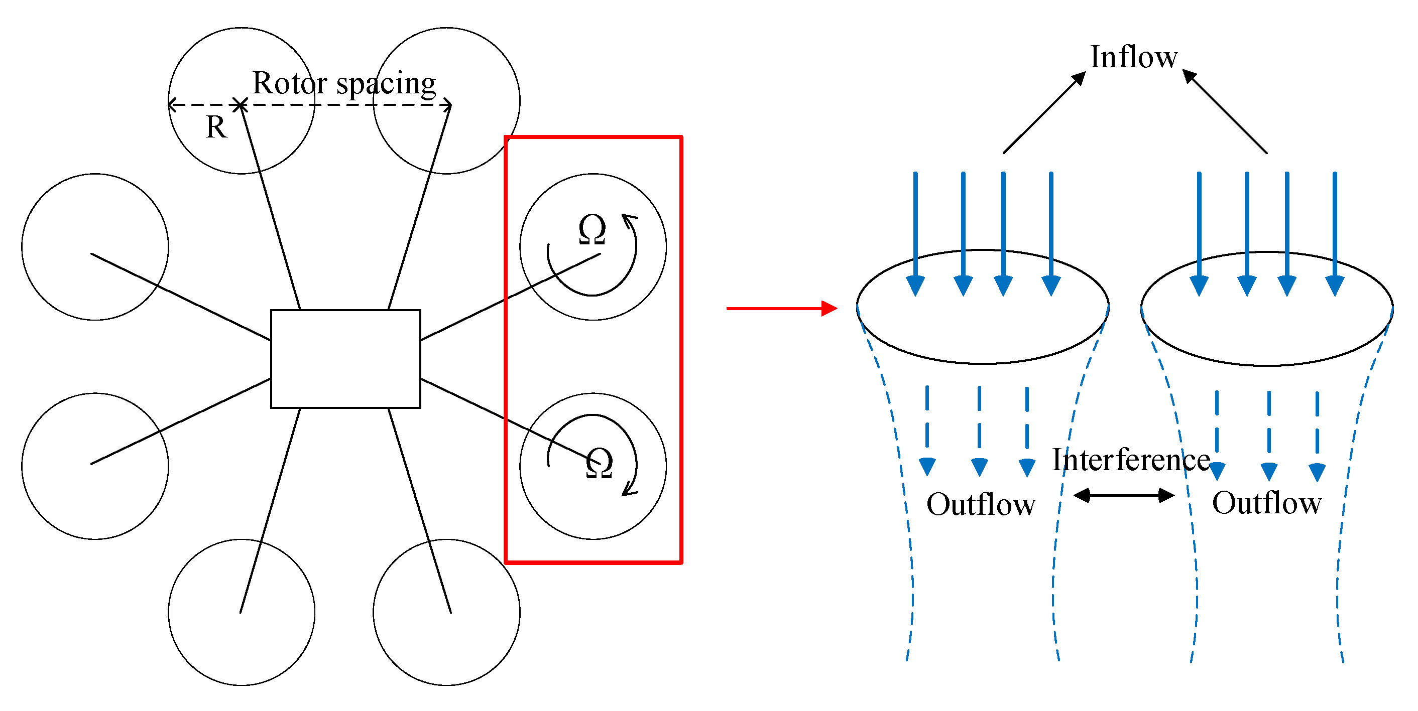
2. Theoretical Analysis

Momentum theory is assumed to be an effective method for flow-field analysis of rotorcrafts. It regards the rotating rotor as an actuator disk and relates the induced airflow velocity through the actuator disk to the thrust and power of the rotor. According to the momentum theory [23], the induced flow velocity can be expressed as:

$$V_h=\sqrt{T/2\rho A}$$

(1)

where T is the thrust generated by the rotor, $\rho$ is the air density, with a value of $1.225 \mathrm{kg}\cdot {\mathrm{m}}^{-3}$, and A is the area of the rotor disk.

The induced power consumption can be expressed as:

$$P_i=T{V}_h=T^{3/2}/\sqrt{2\rho A}$$

(2)

To measure the aerodynamic efficiency of a rotor in hover, FM is defined as the ratio of induced power consumption to actual power consumption:

$$FM=\frac{P_i}{P}=\frac{T^{3/2}/\sqrt{2\rho A}}{P}=\frac{C_T^{3/2}/\sqrt{2}}{C_P}$$

(3)

where

$$C_T=\frac{T}{\rho A{\Omega }^2{R}^2}$$

(4)

is the thrust coefficient,

$$C_P=\frac{P}{\rho A{\Omega }^3{R}^3}$$

(5)

is the power coefficient. $\Omega$ is the angular velocity of the rotor and R is the radius of the rotor.

FM of a given rotor is often expressed as a function of $C_T/\sigma$. Here, $\sigma$ is the solidity of the rotor, and can be defined as:

$$\sigma =Nc/\pi R$$

(6)

where N is the number of blades and c is the chord.

Since the tapered blade is adopted in this paper, the influence of varying chord length on the solidity must be considered, and Equation (7) is adopted to calculate the equivalent solidity:

$${\sigma }_e=3{\displaystyle {\int }_0^1\sigma r^2}dr$$

(7)

The total efficiency of the aircraft is determined by the power loading:

$$PL=\frac{T}{P}=\frac{C_T}{C_P\Omega R}$$

(8)

Combined with momentum theory, PL can also be expressed in the following form:

$$PL=\frac{\sqrt{2\rho }FM}{\sqrt{DL}}$$

(9)

where DL is the disk loading and can be defined as:

$$DL=T/A$$

(10)

In addition, the tip chord Reynolds number in this paper is defined by the chord length at 0.75R:

$${\mathrm{Re}}_{tip}=\rho V{c}_{0.75}/\mu$$

(11)

where $\mu$ is kinematic viscosity coefficient of air, with a value of $1.79\times {10}^{-5} \mathrm{Pa}\cdot \mathrm{s}$ with a temperature of 293.15 K, and a pressure of 101.325 kPa.

Figure 1 shows the arrangement of octorotor and interference between adjacent rotors.

3. Hover Experiment

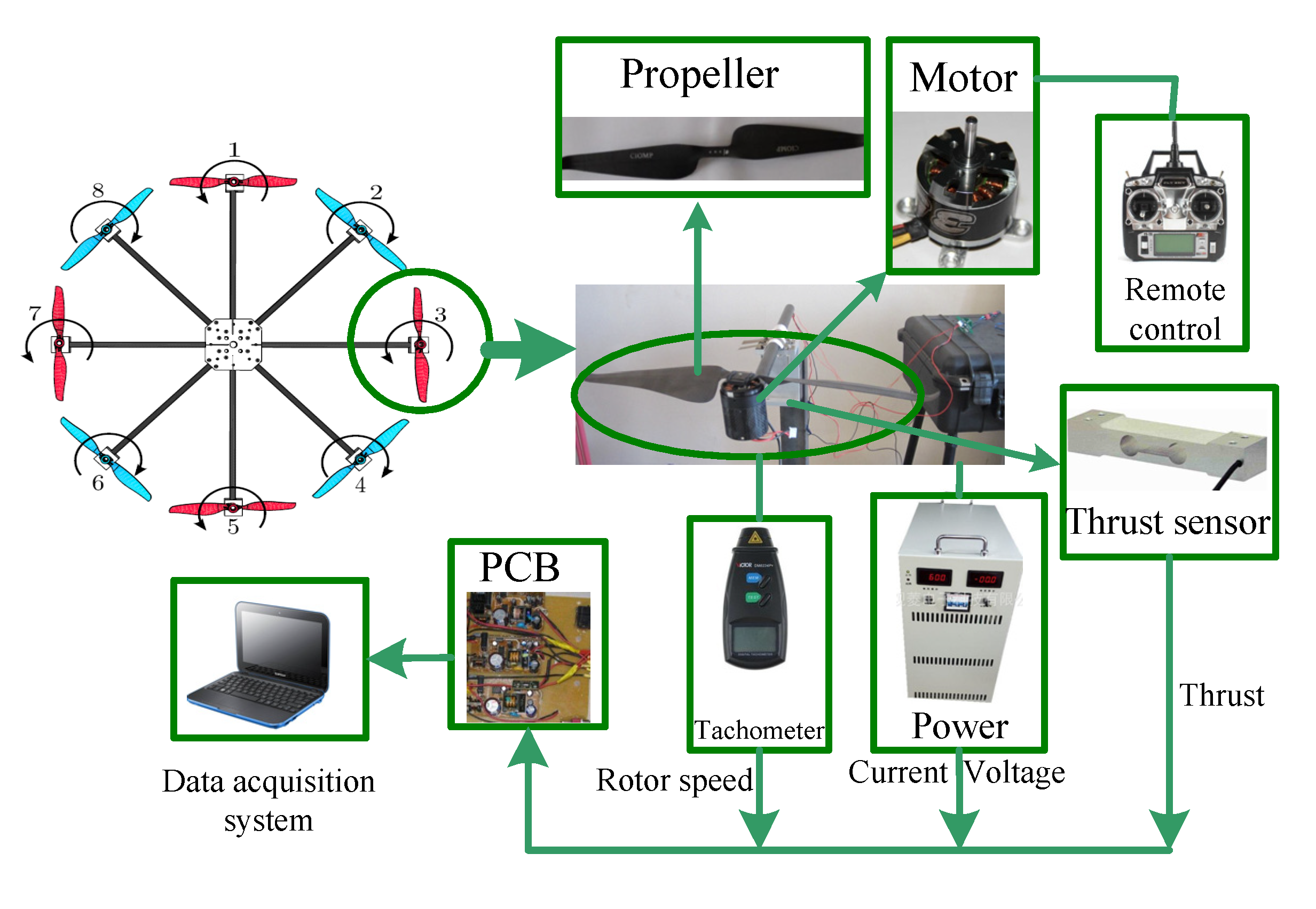
3.1. Experimental Setup

The rotor used in this paper is made of carbon fiber, and unidirectional carbon fiber cloth is used as reinforcement. The weight of one rotor is 15 g. The rotor is operating at Re_tip = 0.59 × 10⁵~0.99 × 10⁵. The specific rotor parameters are shown in

Table 1. Rotor parameters.

Chord (mm)	Radius (m)	Solidity	Pitch (m)	Twist
28	0.2	0.09	0.157	0

.

The schematic diagram of the test bench is shown in Figure 2. Each rotor is fitted with a separate motor and thrust sensors (model CZL601, accuracy ±0.02% F.S., range 0~3 kg). Adjacent rotors rotate in opposite directions, and the rotor speed is measured with an optical tachometer (model DT2234C, accuracy ±0.05 n% + 1 d). To reduce the impact brought by the ground effect, the rotor is installed at a height of 1.5 m above the ground. Rotor spacing L is defined as the distance between the rotor centers of two adjacent rotors. In this experiment, L = 400, 480, 560, 640, and 720 mm, respectively. Thus, the corresponding dimensionless spacing ratios L/D = 1.0, 1.2, 1.4, 1.6, and 1.8 (D is the diameter of the rotor). By changing the tip chord Reynolds number, the thrust and power consumption generated by the octorotor at five spacing are collected, and the aerodynamic performance of the octorotor is analyzed accordingly.

3.2. Error Analysis

The main sources of error in the experiments are the standard deviations of the rotational speed and the mean voltages from the force sensors. Typical values of the standard deviations of thrust are about 1% of the mean values. Rotational speed error is related to the finite number of magnets that excite the tachometer, which causes an error of 1/24 × 60 = 2.5 RPM. The statistical (random) error in the coefficient values for each run was estimated by the standard deviation of repeated samples. This experiment mainly measured variable as thrust T, torque Q, and rotational speed $\Omega$. To determine the accuracy of the test measurements, a normalized criterion is needed in this case [24,25,26]. Consider a variable $X_i$, the uncertainty of the calculated results can be expressed by using the ”Kline–McClintock”’ equation [27]:

$$\Delta R={\left\{{\displaystyle \sum _{i=1}^N{\left(\frac{\partial R}{\partial X_i}\Delta X_i\right)}^2}\right\}}^{1/2}$$

(12)

where $\Delta X_i$ is the uncertainty of $X_i$.

The expression of uncertainty of power can be obtained as follows:

$$\Delta P=\sqrt{{\left(\frac{\partial P}{\partial Q}\Delta Q\right)}^2+{\left(\frac{\partial P}{\partial \Omega }\Delta \Omega \right)}^2}$$

(13)

The uncertainty of P as a percentage is:

$$\frac{\Delta P}{P}=\sqrt{{\left(\frac{\Delta Q}{Q}\right)}^2+{\left(\frac{\Delta \Omega }{\Omega }\right)}^2}$$

(14)

Similarly:

$$\frac{\Delta PL}{PL}=\sqrt{{\left(\frac{\Delta T}{T}\right)}^2+{\left(-\frac{\Delta Q}{Q}\right)}^2+{\left(-\frac{\Delta \Omega }{\Omega }\right)}^2}$$

(15)

$$\frac{\Delta FM}{FM}=\sqrt{{\left(\frac{3}{2}\frac{\Delta T}{T}\right)}^2+{\left(-\frac{\Delta Q}{Q}\right)}^2+{\left(-\frac{\Delta \Omega }{\Omega }\right)}^2}$$

(16)

By calculation, the uncertainty of P, PL, and FM is 1.41%, 1.44%, and 1.51%, respectively. The values of uncertainty that are presented in this study are all calculated for 95% confidence levels.

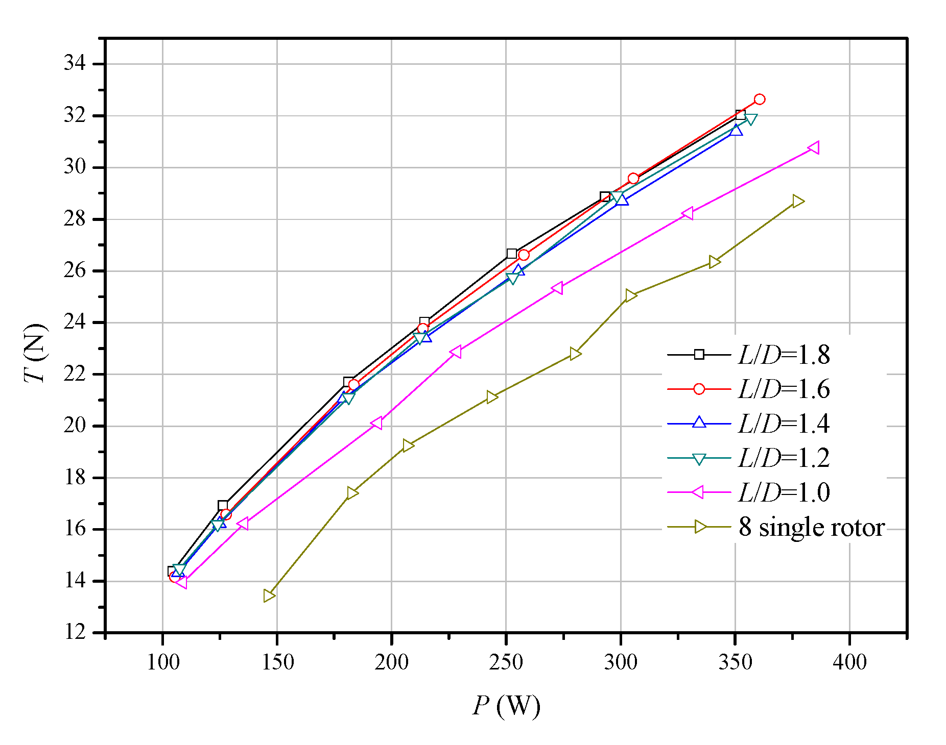
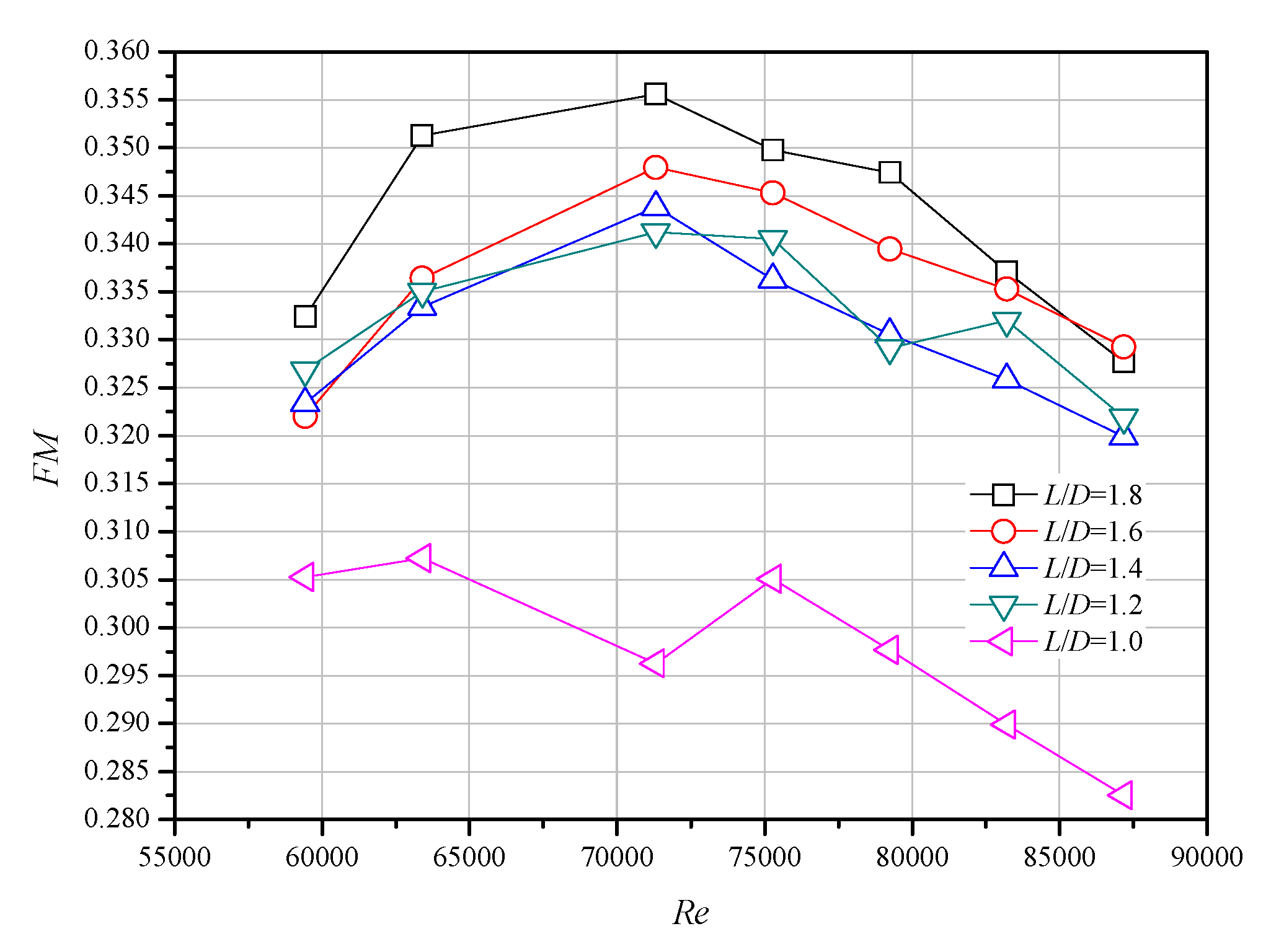
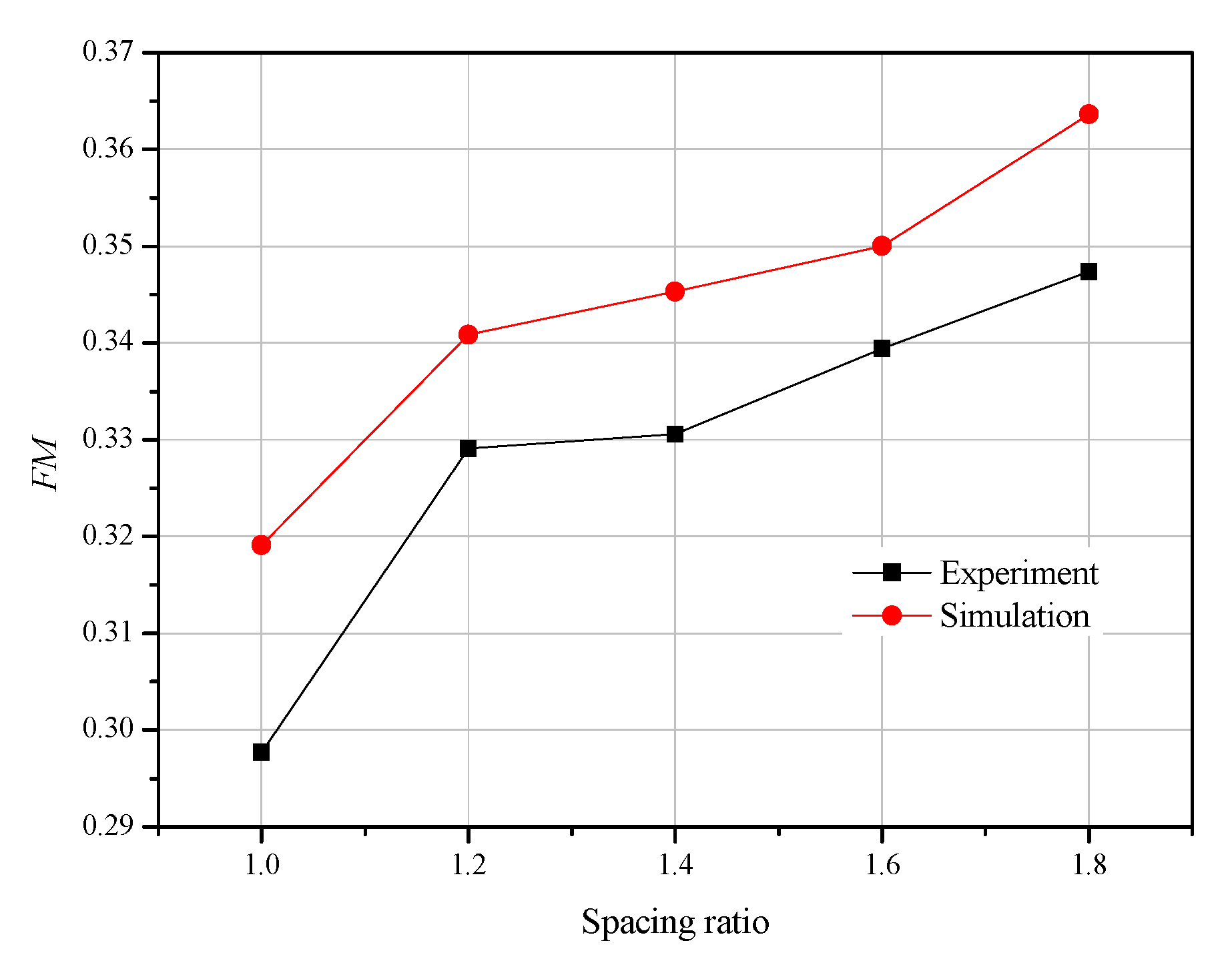
3.3. Results

The thrust and power consumption of the octorotor with different spacing ratios is shown in Figure 3.

It can be seen from Figure 3 that at the same power consumption, the thrust is significantly greater than the simple superposition of the thrust generated by the eight small single rotors. In addition, the thrust generated by the octorotor at L/D = 1.0 is significantly lower than that generated by the octorotor at the other four spacing ratios. It indicates that the rotor interference with proper rotor spacing is beneficial to improve the hover efficiency of the octorotor.

The variation of FM with different rotor spacing ratios is shown in Figure 4.

It can be found from Figure 4 that the FM of the octorotor shares a similar tendency, and it is very interesting to note that there is a sudden drop at Re = 79246 for L/D = 1.2 and at Re = 71,321 for L/D = 1.0. The likeliest explanation for this phenomenon is the collapse of the suction forces on the tip and the increase in vibration caused by the flow separation, which are relatively unsteady for smaller rotor spacing, where the rotor is apt to have somewhat greater interaction with its own wake. This heightened interaction is reflected in the greater variability to a decrease in FM. Furthermore, because of the unpredictable inflow and outflow of smaller rotor spacing where the rotor is apt to have interaction with its own wake, it is, therefore, not entirely surprising that some data do not follow the same trends. Additionally, the aerodynamic performance at L/D = 1.8 is much better than other spacing ratios with a much higher FM.

The variation of power loading versus disk loading is shown in Figure 5.

As can be seen from Figure 5, PL value at L/D = 1.8 always is higher than the other rotor spacings. The PL for 1.4 and 1.2 are approximately the same with a lower value. Especially, the PL for L/D = 1.0 was presented with lowest value which suffered from strong rotor interference.

To sum up, when the spacing ratio is 1.8, the small octorotor has better aerodynamic efficiency and total efficiency, and therefore it can be regarded as the best rotor spacing in the current working condition.

The FM comparison of the small octorotor, the small quadrotor [21], and the small hex-rotor [20] at the optimum rotor spacing is shown in Figure 6.

It can be seen from Figure 6 that the aerodynamic performance of a small octorotor is much better than that of a small quadrotor and a small hex-rotor composed of the same rotor.

4. Numerical Simulation

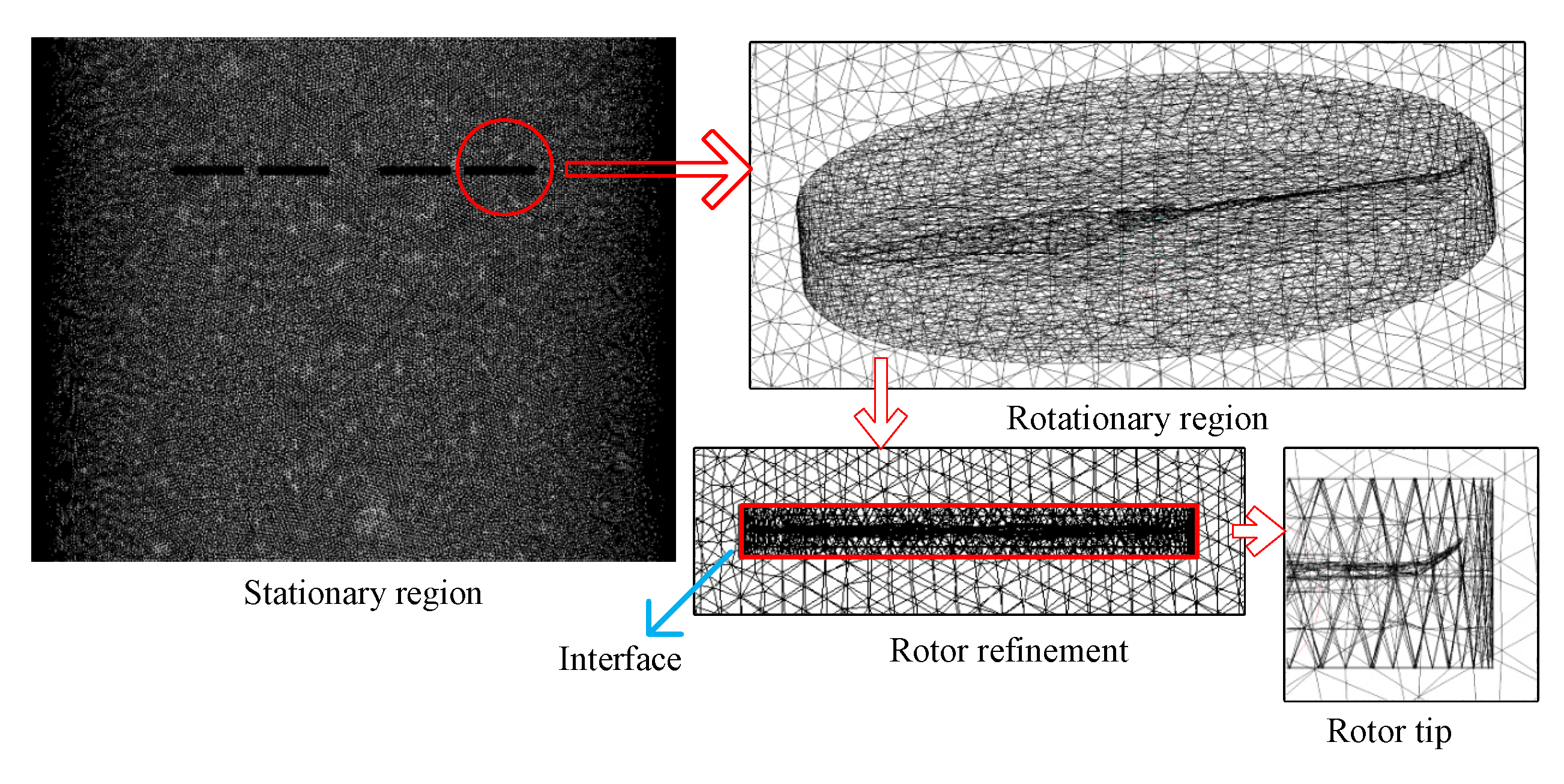
4.1. Simulation Setting and Mesh Analysis

To further analyze the aerodynamic performance of the small octorotor, the flow field of the small octorotor with different spacing ratios was numerically simulated with ANSYS when Re_tip = 0.79 × 10⁵. The detailed mesh distribution is shown in Figure 7.

The whole computational domain is divided into nine regions including one cylinder stationary region and eight cylinder rotating regions (to capture the flow detail of four rotors with refined mesh), which has a total size of 70 million cells. In addition, the SUAV is located in the upper region of the domain to obtain the detail of the downwash flow of the SUAV. To handle the low Reynolds number flows, multiple viscous boundary layers are used in the simulations, and the max element metrics is below 0.8 to capture the flow detail of the rotor tip and the interfaces between stationary and rotating regions. The grid is considered to be sufficient to handle these simulations and the mesh on the rotor tip is refined to reach the independence state. For the boundary conditions, all three surfaces of the cylinder domain are set as no slip wall where the rotating region and stationary overlap is set as interface. The sliding mesh is used for the transient solver. The Spalart–Allmaras turbulence model was chosen for the RANS closure which was proven to be capable of handling the aerodynamic performance of the multi-rotors, especially at low Re. The physical time step corresponds to a rotor rotation of 30 degrees, and 12 steps correspond to a rotor revolution. The rotor made a total of 40 revolutions. Furthermore, the mesh independence study is conducted to show that the results are already reaching the grid independence state.

For the numerical simulation, the accuracy of the model used, the quality of the mesh, the selected boundary conditions, the turbulence model, and the discrete format all produce some errors. For the experiment, the sensor error is the main error source. The comparison between the experimental and simulation results of FM of octorotor is shown in Figure 8.

It can be seen that the simulation results are slightly higher than the experiment, with an error of about 6%, which may be the result of the introduced C_P in experiments and the extra validation of C_P for each simulation to reach the convergence.

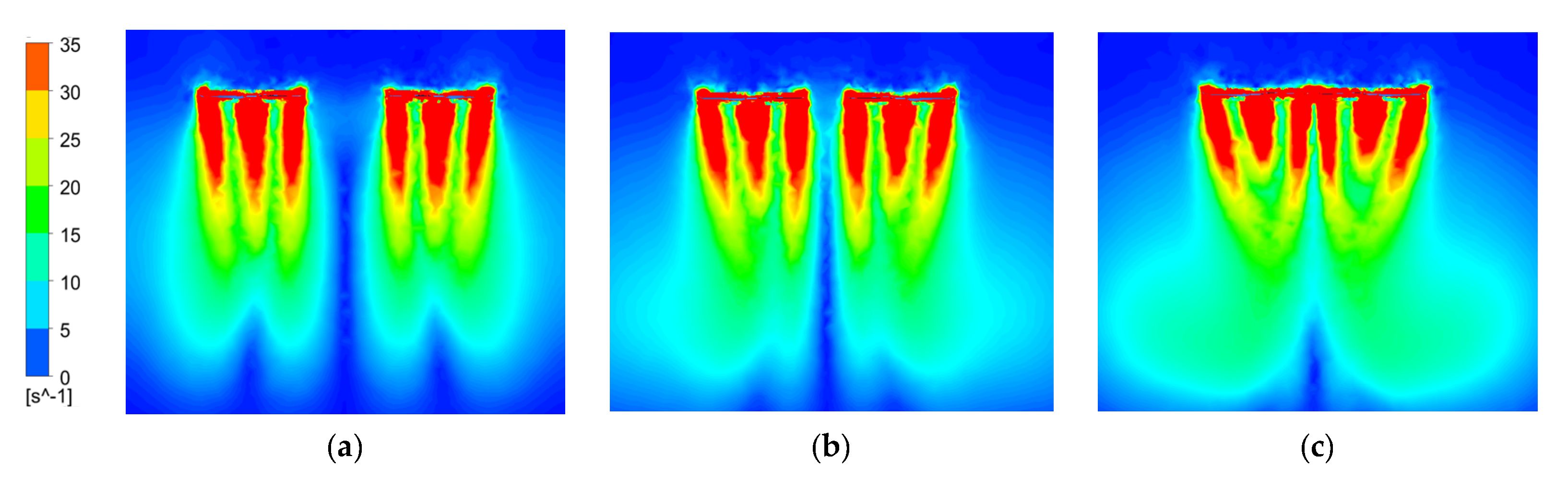
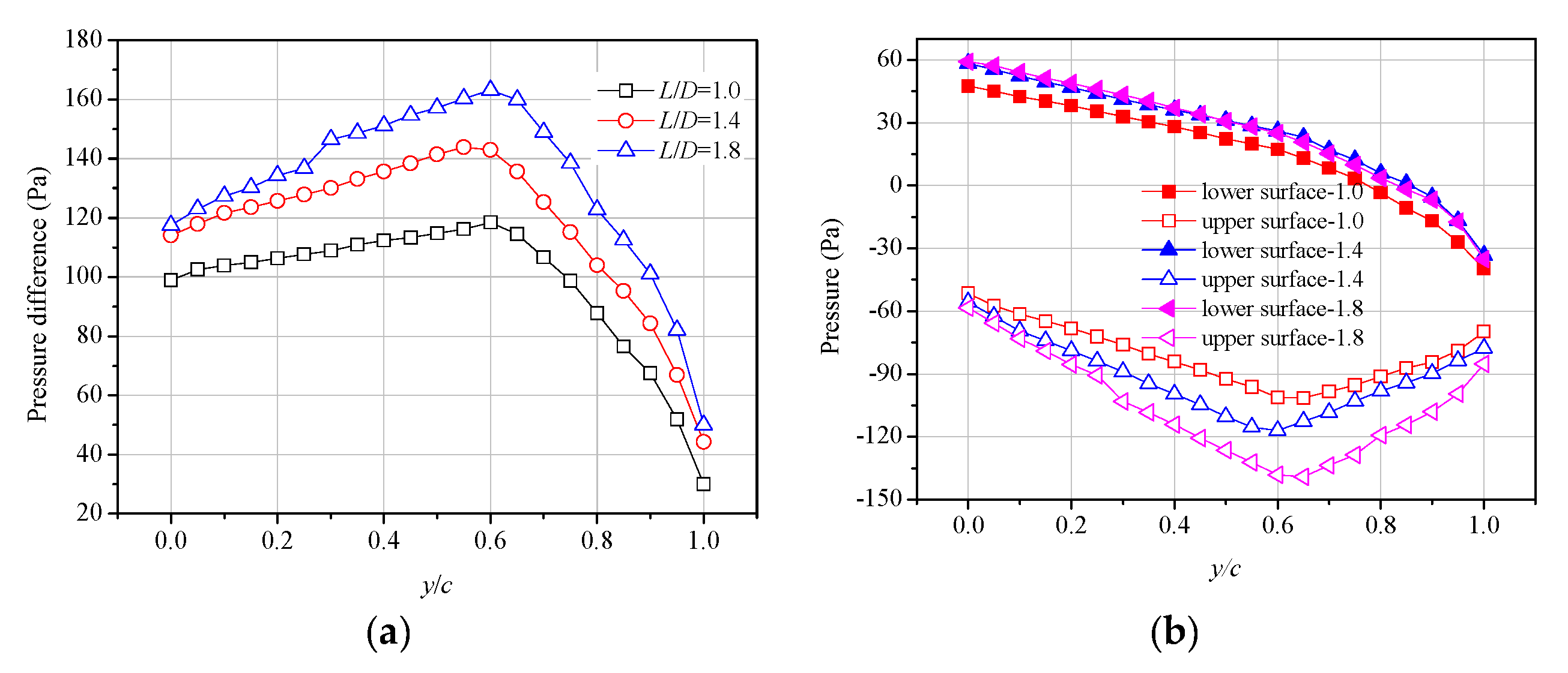
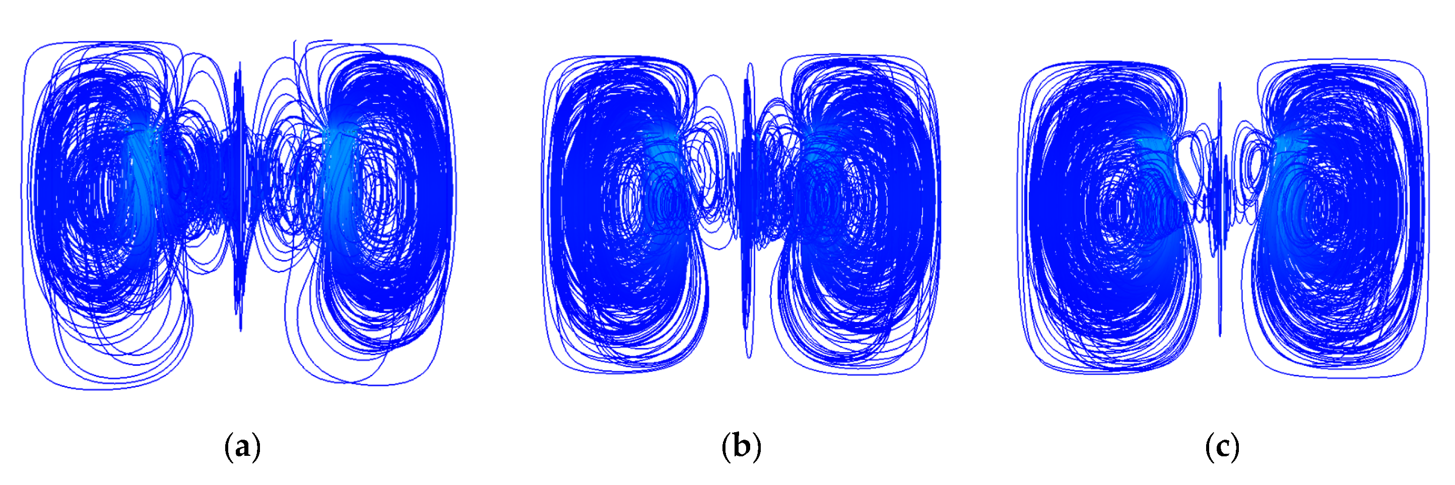
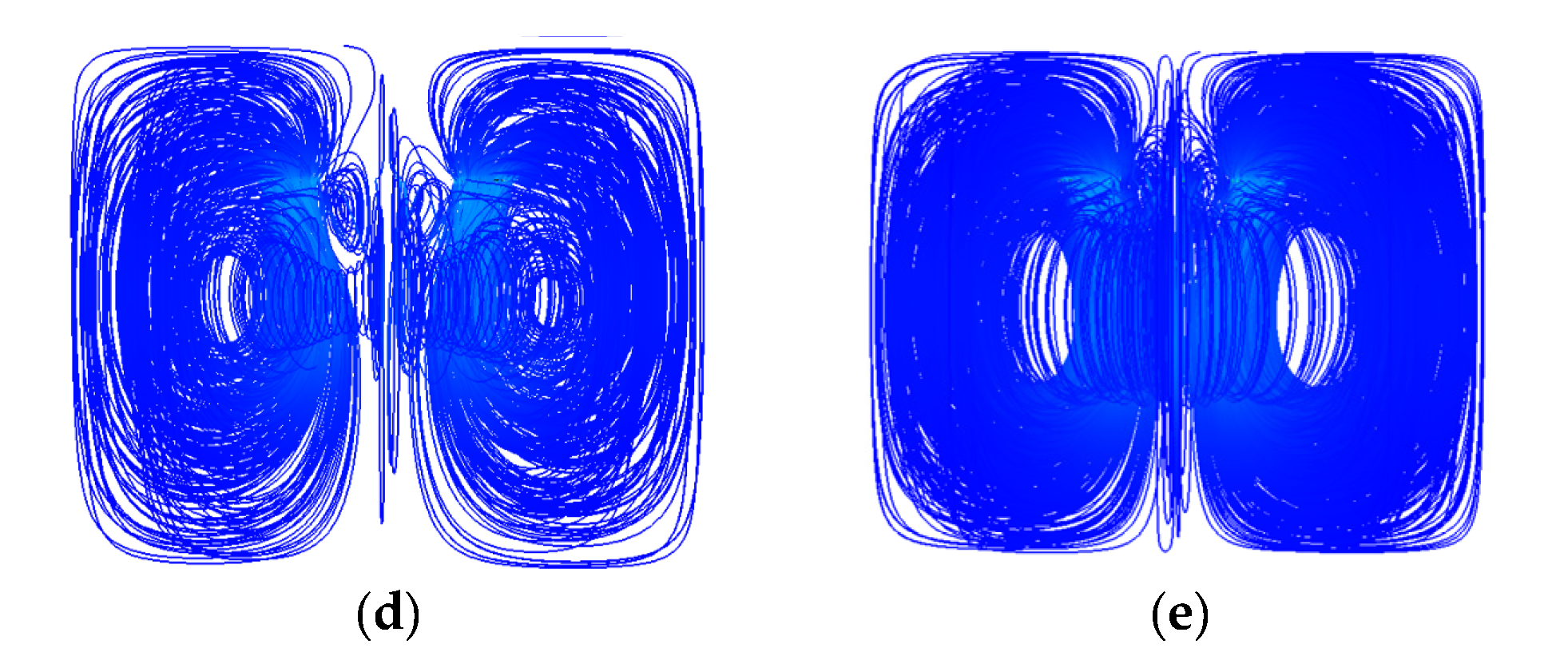
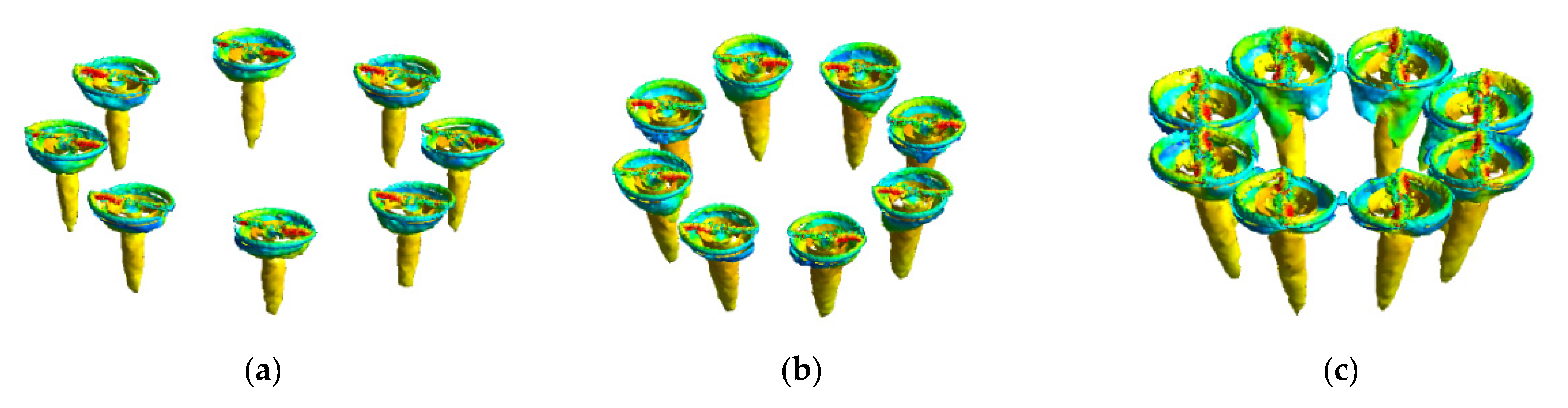
4.2. Simulation Results

The velocity distribution between adjacent rotors with different rotor spacing is shown in Figure 9.

According to Figure 9, it is not difficult to find that rotor wake began to attract each other as the rotor spacing was reduced. Since the wake of each rotor is affected by the wake of the two adjacent rotors, the wake of the rotor shows the phenomenon of inward contraction which may make the rotor unstable and affect the power consumption of the rotor. It also can be found that the vertical vortex below the side of the rotor slowly moves down as the rotor spacing decreases. In addition, the wake of 1.2 and 1.0 appears to be deeper than other spacing ratios, which may make the rotors more susceptible to ground effects.

The vortices distribution between adjacent rotors with different rotor spacing is shown in Figure 10.

Figure 10 shows that the tip vortices and root vortices also attract each other and with a decrease in rotor spacing, the attraction between the vortices becomes more and more intense.

The pressure distribution around the rotor tips with different rotor spacing is shown in Figure 11.

As can be seen from Figure 11a, the pressure difference between the upper and lower surface at the blade tip is intended to decrease with a decrease in rotor spacing. It means a smaller thrust is obtained at smaller spacing. Figure 11b shows that the rotor spacing has a significant effect on the pressure on the upper surface of the rotor tip, but when the spacing is too small (such as L/D = 1.0), the pressure on the lower surface is also affected in this case.

The streamline distribution is shown in Figure 12.

The inward contraction of the rotor wake at 1.2 and 1.0 can be clearly observed from Figure 12d,e which indicates that the thrust and power variations are related to the location and the shape of the vortex.

The Q-criterion for the octorotor with different rotor spacing is shown in Figure 13.

As can be seen in Figure 13, the wake of the rotor shows the phenomenon of inward contraction at L/D = 1.0.

5. Conclusions

To obtain the aerodynamic performance of a small octorotor with different rotor spacing, the small rotor test bench measurements were carried out with CFD simulations. The conclusions are as follows:

• The aerodynamic performance of the rotors change with a change of rotor spacing, but this change is not linear, and therefore it cannot be simply judged that an increase or decrease in the spacing will have a consistent impact on the aerodynamic performance of the rotors. Further analysis is needed to explore the reasons for the influence of rotor spacing on aerodynamic performance and whether or not there is a law that can be expressed mathematically. Nevertheless, through experiments, we found that FM and PL at L/D = 1.8 have obvious advantages as compared with other spacing ratio, which can be regarded as the best spacing ratio under the current working condition, while L/D = 1.0 obviously has a great negative impact on the overall aerodynamic performance due to its too small spacing.
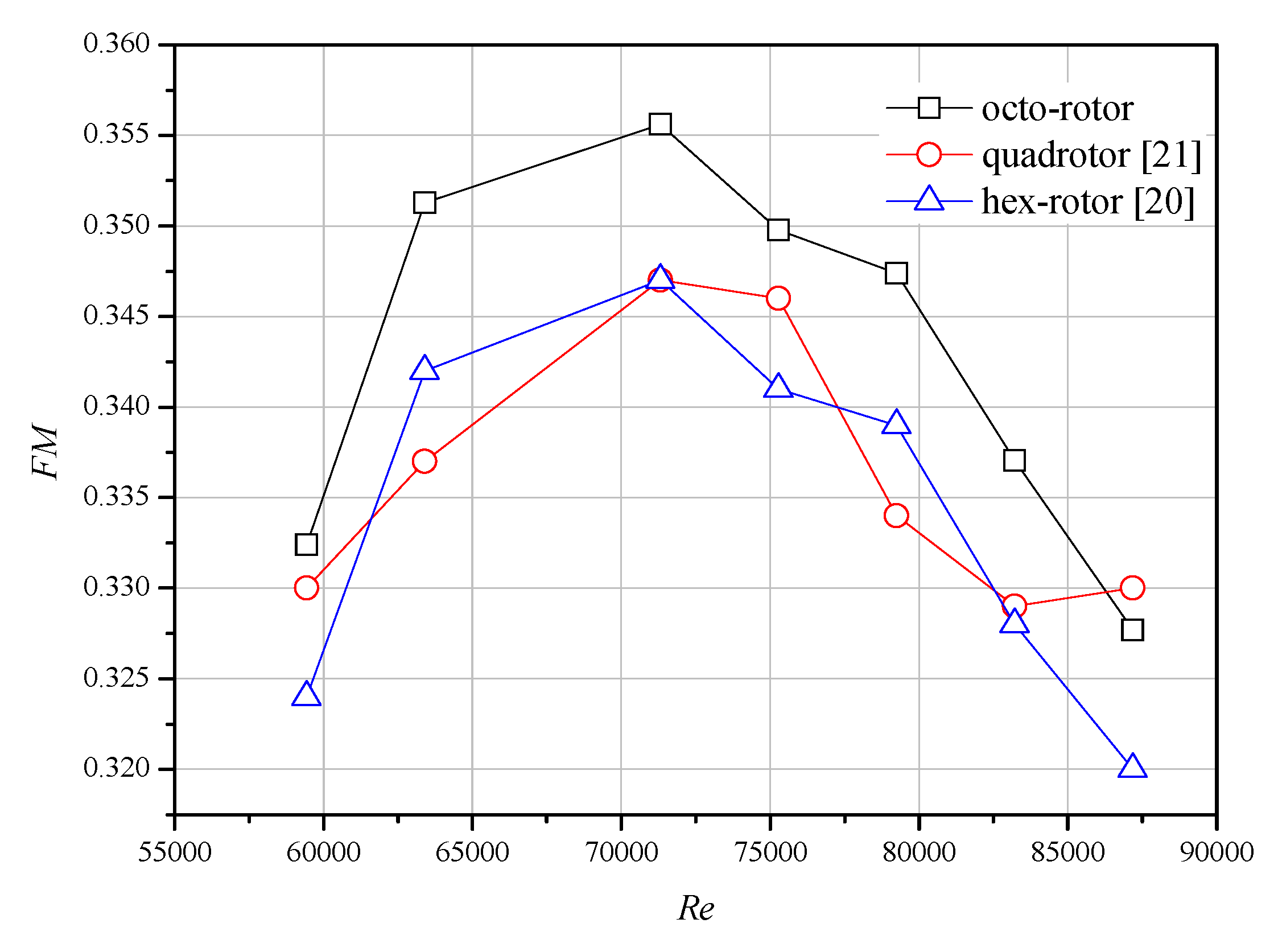
• As compared with eight single rotors, for a quadrotor and hex-rotor with the same rotor size, the FM of octorotor shows a higher value. Especially, L/D = 1.8 was proven to be the optimal rotor spacing with better aerodynamic performance. The configuration of the octorotor helps to increase the aerodynamic performance of the rotors, but at the same time increases the total area of the aircraft, resulting in a higher cost. Therefore, it is necessary to make a tradeoff on rotor arrangement and oversize of the vehicle.
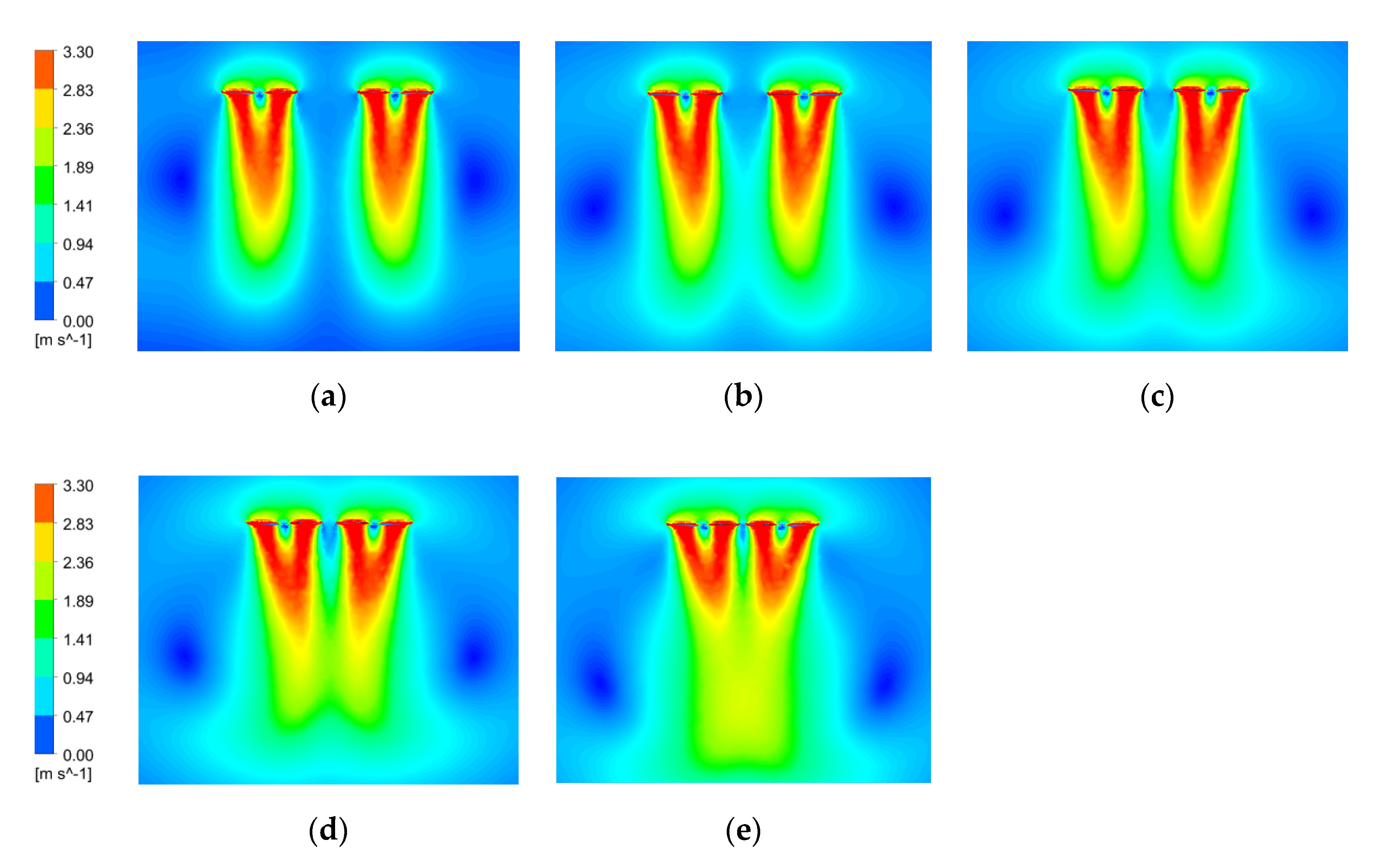
• The numerical simulation results at Re_tip = 0.79 × 10⁵ show that the wake of an octorotor and the vortices of wake attract each other. Moreover, the attraction becomes more obvious as the rotor spacing decreases, which may adversely affect the aerodynamic performance of the rotor. A decrease in rotor spacing will also affect the pressure difference between the upper and lower surfaces of the rotor tips. When the rotor spacing is too small, the pressure difference is sharply reduced, thus affecting the thrust generated. Future work should attempt to obtain an aerodynamic model that considers rotor interference to amend the conventional control theory with application in an octorotor with tilted rotors or wind disturbance.

References

- Lichota, P.; Szulczyk, J. Output Error Method for Tiltrotor Unstable in Hover. Arch. Mech. Eng. 2017, 64. [Google Scholar] [CrossRef] [Green Version]
- Mettler, B.; Tischler, M.; Kanade, T.M.; Kanade, T. System Identification of Small-Size Unmanned Helicopter Dynamics. In Proceedings of the 55th Annual Forum of the American Helicopter Society, Montreal, QC, Canada, 25–27 May 1999; pp. 1706–1717. [Google Scholar]
- Hrishikeshavan, V.; Benedict, M.; Chopra, I.H.; Chopra, I. Identification of Flight Dynamics of a Cylcocopter Micro Air Vehicle in Hover. J. Aircr. 2015, 52, 116–129. [Google Scholar] [CrossRef]
- Zhang, S.; Yang, B.; Xie, H.; Song, M. Applications of an Improved Aerodynamic Optimization Method on a Low Reynolds Number Cascade. Processes 2020, 8, 1150. [Google Scholar] [CrossRef]
- Bohorquez, F.; Pines, D. Hover Performance of Rotor Blades at Low Reynolds Numbers for Rotary Wing Micro Air Vehicles. In Proceedings of the 21st AIAA Applied Aerodynamics Conference, Orlando, FL, USA, 23–26 June 2003. [Google Scholar]
- Bohorquez, F.; Samuel, P.; Sirohi, J.; Pines, D.; Rudd, L.; Perel, R. Design, Analysis and Hover Performance of a Rotary Wing Micro Air Vehicle. J. Am. Helicopter Soc. 2003, 48, 80–90. [Google Scholar] [CrossRef] [Green Version]
- Bohorquez, F.; Pines, D.; Samuel, P.D. Small Rotor Design Optimization Using Blade Element Momentum Theory and Hover Tests. J. Aircr. 2010, 47, 268–283. [Google Scholar] [CrossRef]
- Ramasamy, M.; Johnson, B.; Leishman, J.G. Understanding the Aerodynamic Efficiency of a Hovering Micro-Rotor. J. Am. Helicopter Soc. 2008, 53, 412–428. [Google Scholar] [CrossRef]
- Lakshminarayan, K.V.; Baeder, J.D. High-Resolution Computational Investigation of Trimmed Coaxial Rotor Aerodynamics in Hover. J. Am. Helicopter Soc. 2009, 54, 42008. [Google Scholar] [CrossRef]
- Syal, M.; Leishman, G.J. Aerodynamic Optimization Study of a Coaxial Rotor in Hovering Flight. J. Am. Helicopter Soc. 2012, 57, 1–15. [Google Scholar] [CrossRef]
- Yoon, S.; Chaderjian, N.; Pulliam, H.T.; Holst, T. Effect of Turbulence Modeling on Hovering Rotor Flows. In Proceedings of the 45th AIAA Fluid Dynamics Conference, Dallas, TX, USA, 22–26 June 2015. [Google Scholar]
- Diaz, V.P.; Yoon, S. High-Fidelity Computational Aerodynamics of Multi-Rotor Unmanned Aerial Vehicles. In Proceedings of the 2018 AIAA Aerospace Sciences Meeting, Kissimmee, FL, USA, 8–12 January 2018. [Google Scholar]
- Yoon, S.; Lee, C.H.; Pulliam, H.T. Computational Analysis of Multi-Rotor Flows. In Proceedings of the 54th AIAA Aerospace Sciences Meeting, San Diego, CL, USA, 4–8 January 2016. [Google Scholar]
- Henricks, Q.; Wang, Z.; Zhuang, M.H.; Zhuang, M. Small-Scale Rotor Design Variables and Their Effects On Aerodynamic and Aeroacoustic Performance of a Hovering Rotor. J. Fluids Eng. 2020, 142. [Google Scholar] [CrossRef]
- Wang, Z.; Henricks, Q.; Zhuang, M.; Pandey, A.; Sutkowy, M.; Harter, B.; McCrink, M.; Gregory, J. Impact of Rotor–Airframe Orientation on the Aerodynamic and Aeroacoustic Characteristics of Small Unmanned Aerial Systems. Drones 2019, 3, 56. [Google Scholar] [CrossRef] [Green Version]
- Shukla, D.; Hiremath, N.; Patel, S.; Komerath, N. Aerodynamic Interactions Study on Low-Re Coaxial and Quad-Rotor Configurations. In Proceedings of the ASME 2017 International Mechanical Engineering Congress and Exposition, Tampa, FL, USA, 3–9 November 2017. [Google Scholar]
- Shukla, D.; Komerath, N. Low Reynolds number multirotor aerodynamic wake interactions. Exp. Fluids 2019, 60. [Google Scholar] [CrossRef]
- Zhang, X.; Xu, W.; Shi, Y.; Cai, M.; Li, F. Study on the effect of tilting-rotor structure on the lift of small tilt rotor aircraft. In Proceedings of the 2017 2nd International Conference on Advanced Robotics and Mechatronics, Hefei, China, 27–31 August 2017; pp. 380–385. [Google Scholar]
- Yang, S.; Liu, X.; Bingtai, C.; Li, S.; Zheng, Y. CFD Models and Verification of the Downwash Airflow of an Eight-rotor UAV. In Proceedings of the 2019 ASABE Annual International Meeting, Boston, MA, USA, 7–10 July 2019. [Google Scholar]
- Lei, Y.; Wang, H. Aerodynamic Optimization of a Micro Quadrotor Aircraft with Different Rotor Spacings in Hover. Appl. Sci. 2020, 10, 1272. [Google Scholar] [CrossRef] [Green Version]
- Lei, Y.; Wang, J. Aerodynamic Performance of Quadrotor UAV with Non-Planar Rotors. Appl. Sci. 2019, 9, 2779. [Google Scholar] [CrossRef] [Green Version]
- Lei, Y.; Cheng, M. Aerodynamic performance of a Hex-rotor unmanned aerial vehicle with different rotor spacing. Meas. Control 2020, 53, 002029401990131. [Google Scholar] [CrossRef] [Green Version]
- Johnson, W. Helicopter Theory; Courier Dover Publications: New York, NY, USA, 1994. [Google Scholar]
- Lichota, P. Inclusion of the D-optimality in multisine manoeuvre design for aircraft parameter estimation. J. Theor. Appl. Mech. 2016, 54, 87–98. [Google Scholar] [CrossRef] [Green Version]
- Tischler, M.B.; Remple, R.K. Aircraft and Rotorcraft System Identification, 2nd ed.; American Institute of Aeronautics and Astronautics: Reston, VA, USA, 2012. [Google Scholar]
- Jategaonkar, R.V. Flight Vehicle System Identification: A Time Domain Methodology, 2nd ed.; American Institute of Aeronautics and Astronautics: Reston, VA, USA, 2015. [Google Scholar]
- Kline, S.; McClintock, F. Describing Uncertainties in Single-Sample Experiments. J. Mech. Eng. 1953, 75, 3–8. [Google Scholar]