Thermal Radiation and MHD Effects in the Mixed Convection Flow of Fe₃O₄–Water Ferrofluid towards a Nonlinearly Moving Surface

Abstract

This paper investigated the magnetohydrodynamic (MHD) mixed convection flow of Fe₃O₄-water ferrofluid over a nonlinearly moving surface. The present work focused on how the state of suction on the surface of the moving sheet and the effects of thermal radiation influence the fluid flow and heat transfer characteristics within the stagnation region. As such, a similarity solution is engaged to transform the governing partial differential equations to the ordinary differential equations. A collocation method, namely the bvp4c function in the MATLAB software solves the reduced system, numerically. Two different numerical solutions were identified for the cases of assisting and opposing flows. The stability analysis was conducted to test the stability of the non-uniqueness solutions. The increment of the thermal radiation effect affects the rate of heat transfer to decrease. The stability analysis conveyed that the upper branch solution is stable and vice versa for the other solution.

1. Introduction

The combined free (natural) and forced convections, also known as mixed convection, normally take place when both free and forced convection mechanisms coexist in order to contribute to both flow and heat transfer. In recent years, many researchers have examined various perspectives of mixed convections in nanofluid as it has numerous industrial significances, especially in nanotechnology. Furthermore, nanofluid refers to an advanced class of heat transfer fluids that consists of nanoparticles and base fluid. On record, Choi [1] initially created the term ‘nanofluid’ in 1995 in an effort to express this new class of fluid. In addition, Saidur et al. [2] indicated that nanofluids are mostly proficient substance with enhanced thermophysical attributes and heat transfer functioning. On top of that, due to tremendous practical interest, a great deal of studies have been conducted to analyze the scope of mixed convection flow and the heat transfer process in nanofluid. For example, a significant analysis was conducted by Ahmad and Pop [3] to examine the mixed convection flow of nanofluid over a vertical surface in a porous medium. Meanwhile, Mahdy [4] discovered the effects of the unsteadiness parameter, mixed convection parameter, Prandtl number, and solid volume fraction of nanoparticles upon unsteady boundary layer flow past an elongating surface in nanofluids. Other than that, Tamim et al. [5] scrutinized the consequences of the mass flux, magnetic field, as well as solid volume fraction of nanoparticles at the moving sheet upon mixed convection stagnation-point flow of a nanofluid. The valuable work of [5] was then extended by Mustafa et al. [6] by incorporating the effects of magnetohydrodynamics and viscous dissipations and concluded that the combination of these effects depreciate the rate of heat transfer. The initiative of Subhashini et al. [7] to solve the problem of mixed convection flow of a nanofluid over an exponentially moving surface is also an excellent effort to fill the research gap within the scope of mixed convection nanofluid flow.

Furthermore, studies referring to thermal radiation effects on both flow and heat transfer in a nanofluid are increasing because nanofluid possesses various properties. Besides, the impact of radiative heat transfer has become progressively significant in designing various advanced energy conversion systems that may operate at high temperatures. Herein, numerous studies have delved into the effects of thermal radiation with varied aspects. For instance, Ibrahim and Shankar [8] explored the presences of heat radiation upon boundary layer flow and heat transfer along with the slip conditions. Meanwhile, in the occurrence of thermal radiation, Yazdi et al. [9] inferred that copper nanoparticles contribute to the highest rate of heat augmentation compared to alumina and titania in a porous medium. Apart from that, Pal and Mandal [10] determined the dominancy of thermal radiation upon mixed convection stagnation-point flow of nanofluid, namely Cu-water, Al₂O₃-water, and TiO₂-water, in a porous medium over a stretching/shrinking surface in the existence of chemical reaction, heat source/sink, and suction/injection. In addition, Pal and Mandal [11] also considered the influences of heat radiation and viscous dissipation on mixed convection flow of nanofluid in a porous medium, and hence managed to identify the dual solutions for the shrinking case. Later, Haroun et al. [12] employed a new method, namely the spectral relaxation method (SRM), to solve the problem of mixed convection flow in MHD nanofluids and produced benchmark solutions, which could be useful for future works.

On the other hand, magnetic nanofluid or ferrofluid, which are also called a special type of nanofluid, refers to a colloidal suspension of magnetic nanoparticles in a non-magnetic base fluid (water, oil, and ethylene glycol) [13]. Note that ferrofluid was pioneered in 1963 at the National Aeronautics and Space Administration (NASA) Research Centre. Following from there, studies on the area of ferrofluid have obtained much interest among researchers due to the numerous applications of ferrofluid in nanotechnology in a wide range of fields related to heat transfer, such as coolant in thermal management devices, heat exchangers, processes that include boiling, and even to improve the cooling function of loud speakers [14,15]. Apart from the applications mentioned above, ferrofluid has been broadly applied in biomedical applications, especially for thermal treatment to battle against tumors and cancers (i.e., hyperthermia) (see [16,17,18] for further details). Hence, due to the enormous practical interest, many researches have been conducted experimentally and numerically to determine the characteristics of flow and heat transfer in a ferrofluid. For example, the experimental study on convective heat transfer of ferrofluid in the existence of a magnetic field led to the uncovering of the fact that the heat transfer enhancement of ferrofluid was proven noteworthy in the presence of magnetic fields, primarily due to the changes in ferrofluid’s thermophysical properties [19]. In another empirical study, it was discovered that the thermal conductivity enhancement of ferrofluid under a magnetic field presented great potential for coolant applications under a controlled magnetic field [20]. On the other hand, Khan et al. [21] numerically studied the MHD stagnation-point flow and heat transfer towards a stretching sheet in a ferrofluid with viscous dissipation. Besides, Mustafa et al. [22] numerically studied the stagnation point flow and heat transfer of a ferrofluid past a stretchable rotating disk with a magnetic field. Later on, Ilias et al. [23] deliberated the MHD natural convection boundary layer flow and heat transfer of a ferrofluid past a vertical semi-infinite flat plate. In another study, Abbas and Sheikh [24] examined the homogeneous–heterogeneous reactions on stagnation-point flow of a ferrofluid past a flat horizontal surface in the existence of an external magnetic field and non-linear slip boundary condition. Apart from that, the impacts of radiation, viscous dissipation, and velocity slip upon ferrofluid flow over a slandering stretching sheet with an aligned magnetic field were investigated by [25]. On the other hand, the impacts of thermal radiation, magnetic field, and viscous dissipation upon ferrofluid flow were examined over a nonlinearly stretching sheet in a convective condition [26]. From the outcome of the literature review, it was found that the effect of thermal radiation in the mixed convection ferrofluid flow past a stretching/shrinking sheet, with the identification of the dual solutions and its stability, has not been investigated yet. Therefore, the present work attempts to reconsider the work of Shen et al. [27], which solved the problem of MHD mixed convection stagnation-point flow past the nonlinearly vertical stretching sheet with the presence of the velocity slip, by considering the influence of the thermal radiation, excluding the velocity slip, and focusing on the state of the shrinking in a water-based magnetite (Fe₃O₄) ferrofluid. We employed the mathematical nanofluid model suggested by Tiwari and Das [28]. Interestingly, the flow of this special type of nanofluid was studied in the cases of assisting and opposing flows in the existence of suction. In addition, stability analysis, which has been gaining much attention among researchers [29,30,31,32,33,34,35,36], was performed for dual solutions. Hence, it is believed that the current numerical results are original and distinguished by Shen et al. [27]. There are many approaches that can be used to solve the convection fluid flow and heat transfer problems, for instance, the classical density functional theory (DFT) method [37] and Poisson–Boltzmann (PB) theory [38]. However, the present problem was solved via the collocation method, namely the bvp4c function in the MATLAB, due to its efficiency in producing more than one numerical solution. Thus, the numerical solutions that reflect the behavior of the fluid flow and heat transfer are presented and will be discussed in detail.

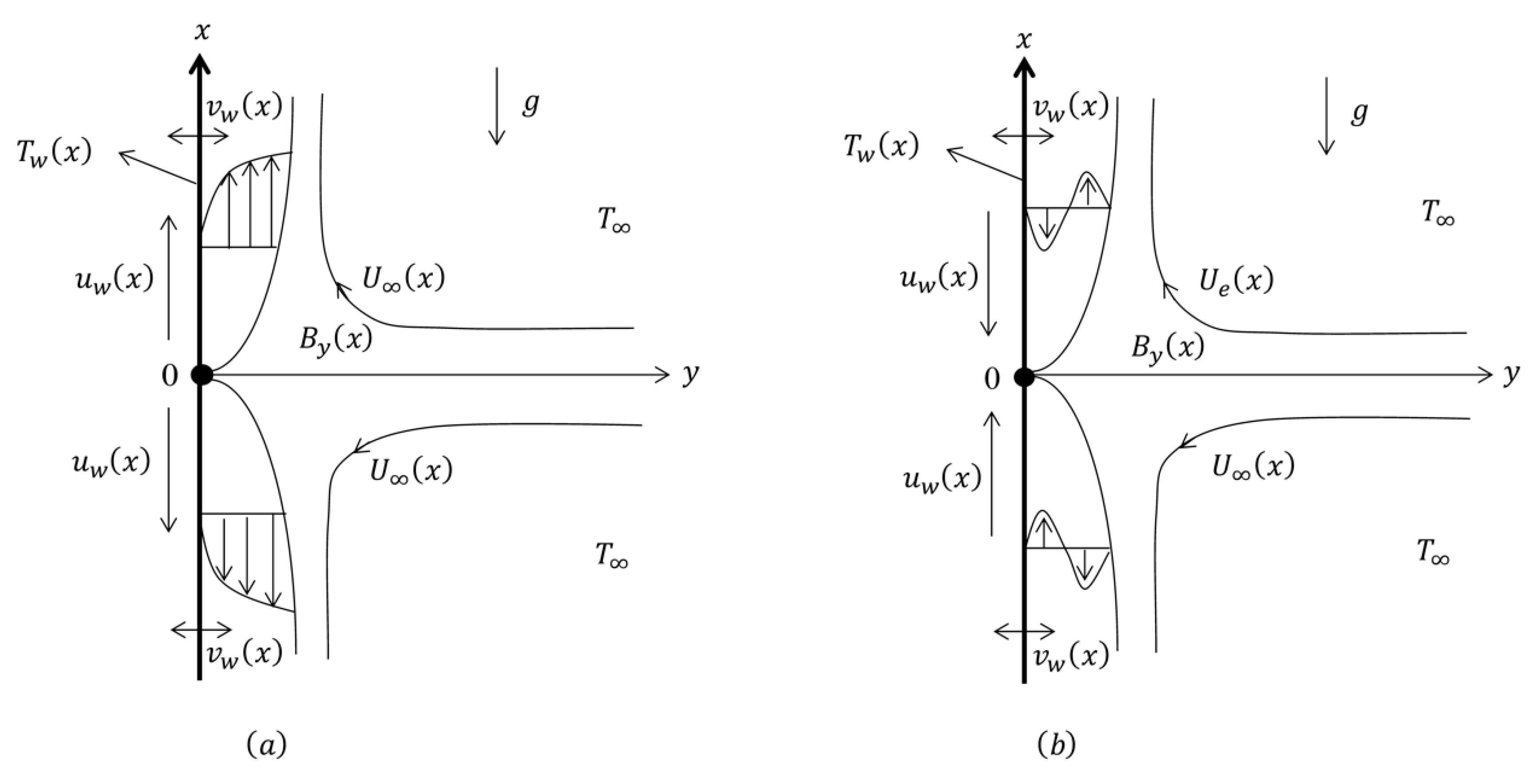
2. Formulation of the Problem

The present work deliberated the steady, two-dimensional mixed convection flow and heat transfer of a viscous and incompressible electrically conducting fluid over a penetrable nonlinearly stretching/shrinking sheet. The sheet was positioned vertically. The flow geometry is schematically displayed in Figure 1. The fluid refers to the water-based ferrofluid, which consisted of magnetite (Fe₃O₄) nanoparticles. The flow was under the effects of thermal radiation and a transverse magnetic field of strength B, which was assumed for application in the positive y-direction normal to the sheet. In view of the current study, it was assumed that the induced magnetic field was negligible. Besides, it was also assumed that the velocity of the flow external to the boundary layer was $u_e\left(x\right)$, the velocity of the wall mass flux was $v_w\left(x\right)$, the temperature of the sheet was $T_w\left(x\right)$, and the ambient temperature was $T_{\infty }$. Furthermore, the sheet was assumed to stretch/shrink continuously in the x-direction with a velocity of $u_w\left(x\right)$.

Under these assumptions, along with the Boussinesq and the boundary layer approximations, the governing partial differential equations of the problem were given as below (Shen et al. [27] and Tiwari and Das [28]):

$$\frac{\partial u}{\partial x}+\frac{\partial v}{\partial y}=0,$$

(1)

$$u\frac{\partial u}{\partial x}+v\frac{\partial u}{\partial y}=u_e\frac{d{u}_e}{dx}+\frac{{\mu }_{nf}}{{\rho }_{nf}}\frac{{\partial }^{2}u}{\partial y^2}+\frac{{\sigma }_{nf}{B}_y^2}{{\rho }_{nf}}\left(u_e-u\right)+\frac{{\left(\rho \beta \right)}_{nf}}{{\rho }_{nf}}\left(T-T_{\infty }\right)g,$$

(2)

$$u\frac{\partial T}{\partial x}+v\frac{\partial T}{\partial y}={\alpha }_{n\text{}f}\frac{{\partial }^2\text{}T}{\partial y^2}-\frac{1}{{\left(\rho C_p\right)}_{n\text{}f}}\frac{\partial q_r}{\partial y},$$

(3)

subject to the boundary conditions:

$$\begin{array}{l}u=u_w\left(x\right),v=v_w\left(x\right),T=T_w\left(x\right)\mathrm{at}y=0,\\ u\to u_e\left(x\right),T\to T_{\infty }\mathrm{as}y\to \infty ,\end{array}$$

(4)

where u and v represent the velocity components along the x and y directions, respectively, g is the acceleration due to gravity, $B_y\left(x\right)$ refers to the magnetic field, T denotes the temperature of the ferrofluid, $q_r$ reflects the radiation heat flux, ${\nu }_{n\text{}f}$ denotes the kinematic viscosity of the ferrofluid, ${\sigma }_{n\text{}f}$ is the electrical conductivity of the ferrofluid, ${\rho }_{n\text{}f}$ refers to the density of the ferrofluid, $\left(\rho \beta \right){}_{n\text{}f}$ reflects the thermal expansion coefficient of the ferrofluid, ${\alpha }_{n\text{}f}$ denotes the thermal diffusivity of the ferrofluid, ${\mu }_{n\text{}f}$ represents the dynamic viscosity of the ferrofluid, as described in the Brinkman’s model, and lastly, ${\left(\rho C_p\right)}_{n\text{}f}$ represents the heat capacitance of the ferrofluid. The effective properties of the ferrofluid are further described in the following (see [39,40]):

$$\begin{array}{l}{\mu }_{n\text{}f}=\frac{{\mu }_f}{{\left(1-\varphi \right)}^{2.5}},{\alpha }_{n\text{}f}=\frac{k_{n\text{}f}}{{\left(\rho C_p\right)}_{n\text{}f}},{\rho }_{n\text{}f}=\left(1-\varphi \right){\rho }_f+\varphi {\rho }_s,\\ {\left(\rho \beta \right)}_{n\text{}f}=\left(1-\varphi \right){\left(\rho \beta \right)}_f+\varphi {\left(\rho \beta \right)}_s,{\left(\rho C_p\right)}_{n\text{}f}=\left(1-\varphi \right){\left(\rho C_p\right)}_f+\varphi {\left(\rho C_p\right)}_s,\\ \frac{{\sigma }_{n\text{}f}}{{\sigma }_{\text{}f}}=1+\frac{3\left({\sigma }_s/{\sigma }_f-1\right)\varphi }{{\sigma }_s/{\sigma }_f+2-\left({\sigma }_s/{\sigma }_f-1\right)\varphi },\frac{k_{n\text{}f}}{k_f}=\frac{k_s+2k_f-2\varphi \left(k_f-k_s\right)}{k_s+2k_f+\varphi \left(k_f-k_s\right)},\end{array}$$

(5)

where ${\mu }_{\text{}f}$ signifies the base fluid’s dynamic viscosity, $\varphi$ connotes the nanoparticle solid volume fraction, ${\rho }_f$ and ${\rho }_s$ symbolize the density of the base fluid and the solid nanoparticle, respectively, $k_{n\text{}f}$ is the ferrofluid thermal conductivity, where the subscript ‘f’ represent the base fluid while ‘s’ denotes the nanoparticle.

Next, applying the Rosseland’s approximation, the radiation heat flux, $q_r$, possesses the following form given by:

$$q_r=-\frac{4\sigma *}{3k*}\frac{\partial T^4}{\partial y},$$

(6)

where $\sigma *$ is the Stefan–Boltzmann constant and $k\text{}*$ denotes the Rosseland mean spectral absorption coefficient. The differences in the temperature within the flow vicinity are assumed to be $T^4$, which can be expanded in a Taylor’s series as a linear combination of the temperature. Upon expanding $T^4$ into the Taylor’s series for $T_{\infty }$, it was approximated after neglecting the higher order terms, yielding $T^4=4T_{\infty }^{3}T-3T_{\infty }^4$. Thus, Equation (3) is reduced as:

$$u\frac{\partial T}{\partial x}+v\frac{\partial T}{\partial y}={\alpha }_{n\text{}f}\frac{{\partial }^{2}T}{\partial y^2}+\frac{16\sigma *T_{\infty }^3}{3k*{\left(\rho C_p\right)}_{nf}}\frac{{\partial }^2\text{}T}{\partial y^2}.$$

(7)

Next, in order to obtain the similarity solutions of the governing Equations (1), (2) and (7), which are subjected to the boundary conditions (4), expressions $u_w\left(x\right)$, $v_w\left(x\right)$, $T_w\left(x\right)$, $u_e\left(x\right)$, and $B_y\left(x\right)$ are presented in the following form:

$$\begin{array}{l}{u}_w\left(x\right)=b{x}^n,v_w\left(x\right)=-\frac{n+1}{2}\sqrt{a{\nu }_f}{x}^{\left(n-1\right)/2}s,T_w\left(x\right)=T_{\infty }+T_0{x}^{2n-1},\\ u_e\left(x\right)=a{x}^n,B_y\left(x\right)=B_0{x}^{\left(n-1\right)/2}.\end{array}$$

(8)

Here, a and b are constants, $B_0$ is the characteristic magnetic field, n functions as the positive constant, s is the suction parameter, and $T_0$ is the constant characteristic temperature, with $T_0<0$ signifying a cooled surface (opposing flow) and $T_0>0$ corresponding to a heated surface (assisting flow).

In this study, the similarity transformation is defined as follows (Shen et al. [27]):

$$\begin{array}{l}u=a{x}^n{f}^{\prime }\left(\eta \right),v=-\sqrt{a{\nu }_f}{x}^{\left(n-1\right)/2}\left[\frac{n+1}{2}\text{}f\left(\eta \right)+\frac{n-1}{2}\eta f^{\prime }\left(\eta \right)\right],\\ \theta \left(\eta \right)=\frac{T-T_{\infty }}{T_w-T_{\infty }},\eta =\sqrt{\frac{a}{{\nu }_f}}{x}^{\left(n-1\right)/2}y.\end{array}$$

(9)

The substitution of Equation (9) into Equations (2) and (7) provides:

$$\frac{1}{{\left(1-\varphi \right)}^{2.5}}{f}^{‴}+\left(1-\varphi +\varphi \frac{{\rho }_s}{{\rho }_f}\right)\left[\frac{n+1}{2}\text{}f\text{}{f}^{″}+n-n{\left(f^{\prime }\right)}^2\right]+\frac{{\sigma }_{n\text{}f}}{{\sigma }_{\text{}f}}M\left(1-f^{\prime }\right)+\left(1-\varphi +\varphi \frac{{\left(\rho \beta \right)}_s}{{\left(\rho \beta \right)}_f}\right)\lambda \theta =0,$$

(10)

$$\frac{1}{\mathrm{Pr}}\left(\frac{k_{n\text{}f}}{k_f}+\frac{4}{3}Nr\right){\theta }^{″}+\left(1-\varphi +\varphi \frac{{\left(\rho C_p\right)}_s}{{\left(\rho C_p\right)}_f}\right)\left[\frac{n+1}{2}\text{}f{\theta }^{\prime }-\left(2n-1\right)f^{\prime }\theta \right]=0,$$

(11)

while the boundary conditions (4) turned to be as follows:

$$\begin{array}{l}f\left(\eta \right)=s,f^{\prime }\left(\eta \right)=c,\theta \left(\eta \right)=1\mathrm{at}\eta =0,\\ f^{\prime }\left(\eta \right)=1,\theta \left(\eta \right)=0\mathrm{as}\eta \to \infty .\end{array},$$

(12)

where M is the magnetic parameter, $\lambda$ refers to the mixed convection parameter, with $\lambda <0$ represents the opposing flow, whereas $\lambda >0$ represents the assisting flow, Pr refers to the Prandtl number, Nr is the thermal radiation parameter, c is the stretching/shrinking parameter, with $c>0$ refers to the stretching sheet and $c<0$ refers to the shrinking sheet, and s is the constant mass flux parameter with s > 0 refers to the suction and s < 0 refers to the injection. The governing parameters M, $\lambda$, Pr, Nr, s, and c can be defined as follows:

$$\begin{array}{l}M=\frac{{\sigma }_f{B}_0^2}{a{\rho }_f},\mathrm{Pr}=\frac{{\nu }_f{\left(\rho C_p\right)}_f}{k_f},\lambda =\frac{G{r}_x}{{\mathrm{Re}}_x^2},\\ Nr=\frac{4\sigma *T_{\infty }^3}{k\text{}*k_f},s=-\left(\frac{2}{n+1}\right)\frac{v_w\left(x\right)}{\sqrt{a{\nu }_f}{x}^{\left(n-1\right)/2}},c=\frac{b}{a},\end{array}$$

(13)

where the local Grashof number, $G{r}_x$, and the local Reynolds number, ${\mathrm{Re}}_x$, are defined as:

$$G{r}_x=\frac{g{\beta }_f\left(T_w-T_{\infty }\right)x^3}{{\nu }_f{}^2},{\mathrm{Re}}_x=\frac{u_{e}x}{{\nu }_f}.$$

(14)

The physical quantities of practical interest are the skin friction coefficient, $C_f$, and the local Nusselt number, $N{u}_x$, defined as follows:

$$C_{f\text{}}=\frac{{\tau }_w}{{\rho }_f{u}_e^2},N{u}_x=\frac{x{q}_w}{k_f\left(T_w-T_{\infty }\right)},$$

(15)

where ${\tau }_w$ is the wall shear stress and $q_w$ denotes the heat flux, given by:

$${\tau }_w={\mu }_{\text{}n\text{}f}{\left(\frac{\partial u}{\partial y}\right)}_{y=0},q_w=-k_{\text{}n\text{}f}{\left(\frac{\partial T}{\partial y}\right)}_{y=0}\text{}+{\left(q_r\right)}_{y=0}.$$

(16)

Substituting Equation (9) into Equations (15) and (16), yields:

$${\mathrm{Re}}_x^{1/2}\text{}{C}_f=\frac{1}{{\left(1-\varphi \right)}^{2.5}}{f}^{″}\left(0\right),{\mathrm{Re}}_x^{-1/2}\text{}N{u}_x=-\left(\frac{k_{n\text{}f}}{k_{\text{}f}}+\frac{4}{3}Nr\right){\theta }^{\prime }\left(0\right).$$

(17)

3. Stability Analysis

The numerical outcomes of the similar Equations (10)–(12) implied the occurrence of two solution branches for the variation of respective governing parameters. Therefore, the stability of the non-uniqueness solutions was tested. The stability of the dual solutions was examined by applying the scheme, as suggested by Merkin [41], Weidman et al. [42], and Harris et al. [43]. The stability analysis was initiated by considering an unsteady problem. Hence, Equation (1) was retained, and Equations (2) and (7) were formed as:

$$\frac{\partial u}{\partial t}+u\frac{\partial u}{\partial x}+v\frac{\partial u}{\partial y}=u_e\frac{d{u}_e}{dx}+\frac{{\mu }_{n\text{}f}}{{\rho }_{n\text{}f}}\frac{{\partial }^{2}u}{\partial y^2}+\frac{{\sigma }_{n\text{}f}{B}_y^2}{{\rho }_{n\text{}f}}\left(u_e-u\right)+\frac{{\left(\rho \beta \right)}_{n\text{}f}}{{\rho }_{n\text{}f}}\left(T-T_{\infty }\right)g,$$

(18)

$$\frac{\partial T}{\partial t}+u\frac{\partial T}{\partial x}+v\frac{\partial T}{\partial y}={\alpha }_{n\text{}f}\frac{{\partial }^2\text{}T}{\partial y^2}+\frac{16\sigma *T_{\infty }^3}{3k\text{}*{\left(\rho C_p\right)}_{n\text{}f}}\frac{{\partial }^2\text{}T}{\partial y^2},$$

(19)

where t denotes the time. In conjunction with the similarity solutions (Equation (9)), the subsequent new similarity transformation was formed:

$$\begin{array}{l}u=a{x}^n\frac{\partial \text{}f}{\partial \eta }\left(\eta ,\tau \right),\\ v=-\sqrt{a{\nu }_f}{x}^{\left(n-1\right)/2}\left[\frac{n+1}{2}\text{}f\left(\eta ,\tau \right)+\frac{n-1}{2}\eta \frac{\partial \text{}f}{\partial \eta }\left(\eta ,\tau \right)+\left(n-1\right)\tau \frac{\partial \text{}f}{\partial \tau }\left(\eta ,\tau \right)\right],\\ \theta \left(\eta ,\tau \right)=\frac{T-T_{\infty }}{T_w-T_{\infty }},\\ \eta =\sqrt{\frac{a}{{\nu }_f}}{x}^{\left(n-1\right)/2}y,\tau =a{x}^{n-1}t.\end{array}$$

(20)

Thus, Equations (18) and (19) were written as given:

$$\begin{array}{l}\frac{1}{{\left(1-\varphi \right)}^{2.5}}\frac{{\partial }^{3}f}{\partial {\eta }^3}+\left(1-\varphi +\varphi \frac{{\rho }_s}{{\rho }_f}\right)[\frac{n+1}{2}\text{}f\frac{{\partial }^{2}f}{\partial {\eta }^2}+n-n{\left(\frac{\partial \text{}f}{\partial \eta }\right)}^2+\left(n-1\right)\tau (\frac{\partial \text{}f}{\partial \tau }\frac{{\partial }^{2}f}{\partial {\eta }^2}\\ -\frac{\partial \text{}f}{\partial \eta }\frac{{\partial }^{2}f}{\partial \eta \partial \tau })-\frac{{\partial }^{2}f}{\partial \eta \partial \tau }]+\frac{{\sigma }_{n\text{}f}}{{\sigma }_f}M\left(1-\frac{\partial \text{}f}{\partial \eta }\right)+\left(1-\varphi +\varphi \frac{{\left(\rho \beta \right)}_s}{{\left(\rho \beta \right)}_f}\right)\lambda \theta =0,\end{array}$$

(21)

$$\begin{array}{l}\frac{1}{\mathrm{Pr}}\left(\frac{k_{n\text{}f}}{k_f}+\frac{4}{3}Nr\right)\frac{{\partial }^2\theta }{\partial {\eta }^2}+\left(1-\varphi +\frac{\varphi {\left(\rho C_p\right)}_s}{{\left(\rho C_p\right)}_f}\right)[\frac{n+1}{2}\text{}f\frac{\partial \theta }{\partial \eta }-\left(2n-1\right)\frac{\partial \text{}f}{\partial \eta }\theta \\ +\left(n-1\right)\tau \left(\frac{\partial \text{}f}{\partial \tau }\frac{\partial \theta }{\partial \eta }-\frac{\partial \text{}f}{\partial \eta }\frac{\partial \theta }{\partial \tau }\right)-\frac{\partial \theta }{\partial \tau }]=0,\end{array}$$

(22)

subject to:

$$\begin{array}{l}f\left(\eta ,\tau \right)=s,\frac{\partial \text{}f}{\partial \eta }\left(\eta ,\tau \right)=c,\theta \left(\eta ,\tau \right)=1\mathrm{at}\eta =0,\\ \frac{\partial \text{}f}{\partial \eta }\left(\eta ,\tau \right)=1,\theta \left(\eta ,\tau \right)=0\mathrm{as}\eta \to \infty .\end{array}$$

(23)

Following from there, to determine the stability of the dual solutions, Weidman et al. [43] was adhered to as follows:

$$f\left(\eta ,\tau \right)=f_0\left(\eta \right)+e^{-\gamma \tau }F\left(\eta ,\tau \right),\theta \left(\eta ,\tau \right)={\theta }_0\left(\eta \right)+e^{-\gamma \tau }G\left(\eta ,\tau \right),$$

(24)

where $\gamma$ is an unknown eigenvalue parameter adopted to determine the linear stability of the flow. Here, $f_0\left(\eta \right)$ and ${\theta }_0\left(\eta \right)$ satisfies the similarity of Equations (10)–(12). Besides, it is worth noting that $F\left(\eta ,\tau \right)$, $G\left(\eta ,\tau \right)$, and all its derivatives are smaller in comparison with $f_0\left(\eta \right)$, ${\theta }_0\left(\eta \right)$ and all its derivatives. Hence, by employing the time-dependent solutions of Equation (24) into Equations (21) and (22), the following expressions can be attained:

$$\begin{array}{l}\frac{1}{{\left(1-\varphi \right)}^{2.5}}\frac{{\partial }^{3}F}{\partial {\eta }^3}+\left(1-\varphi +\varphi \frac{{\rho }_s}{{\rho }_f}\right)[\frac{n+1}{2}\left(f_0\frac{{\partial }^{2}F}{\partial {\eta }^2}+f_0^{″}F\right)-2n\text{}{f}_0^{\prime }\frac{\partial F}{\partial \eta }\\ +\left(n-1\right)\tau \left(\gamma f_0^{\prime }\frac{\partial F}{\partial \eta }-\gamma f_0^{″}F-f_0^{\prime }\frac{{\partial }^{2}F}{\partial \eta \partial \tau }+f_0^{″}\frac{\partial F}{\partial \tau }\right)+\gamma \frac{\partial F}{\partial \eta }-\frac{{\partial }^{2}F}{\partial \eta \partial \tau }]\\ -\frac{{\sigma }_{n\text{}f}}{{\sigma }_f}M\frac{\partial F}{\partial \eta }+\left(1-\varphi +\varphi \frac{{\left(\rho \beta \right)}_s}{{\left(\rho \beta \right)}_f}\right)\lambda G=0,\end{array}$$

(25)

$$\begin{array}{l}\frac{1}{\mathrm{Pr}}\left(\frac{k_{n\text{}f}}{k_f}+\frac{4}{3}Nr\right)\frac{{\partial }^{2}G}{\partial {\eta }^2}+\left(1-\varphi +\varphi \frac{{\left(\rho C_p\right)}_s}{{\left(\rho C_p\right)}_f}\right)[\frac{n+1}{2}\left(f_0\frac{\partial G}{\partial \eta }+F{\theta }_0^{\prime }\right)\\ -\left(2n-1\right)\left(f_0^{\prime }G+{\theta }_0\frac{\partial F}{\partial \eta }\right)+\left(n-1\right)\tau \left(\gamma f_0^{\prime }G-\gamma {\theta }_0^{\prime }F-f_0^{\prime }\frac{\partial G}{\partial \tau }+{\theta }_0^{\prime }\frac{\partial F}{\partial \tau }\right)\\ +\gamma G-\frac{\partial G}{\partial \tau }]=0,\end{array}$$

(26)

subject to:

$$\begin{array}{l}F\left(\eta ,\tau \right)=0,\frac{\partial \text{}F}{\partial \eta }\left(\eta ,\tau \right)=0,G\left(\eta ,\tau \right)=0\mathrm{at}\eta =0,\\ \frac{\partial \text{}F}{\partial \eta }\left(\eta ,\tau \right)=0,G\left(\eta ,\tau \right)=0\mathrm{as}\eta \to \infty .\end{array}$$

(27)

In this study, to determine the early growth or decay of the solutions (Equation (24)), we considered $\tau =0$ [43], which yields $F\left(\eta ,\tau \right)=F_0\left(\eta \right)$ and $G\left(\eta ,\tau \right)=G_0\left(\eta \right).$ Then, the following linearized eigenvalue problem was resolved via the collocation method:

$$\begin{array}{l}\frac{1}{{\left(1-\varphi \right)}^{2.5}}{F}_0^{‴}+\left(1-\varphi +\varphi \frac{{\rho }_s}{{\rho }_f}\right)\left[\frac{n+1}{2}\left(f_0{F}_0^{″}+f_0^{″}{F}_0\right)-\left(2n\text{}{f}_0^{\prime }-\gamma \right)F_0^{\prime }\right]\\ -\frac{{\sigma }_{n\text{}f}}{{\sigma }_f}M{F}_0^{\prime }+\left(1-\varphi +\varphi \frac{{\left(\rho \beta \right)}_s}{{\left(\rho \beta \right)}_f}\right)\lambda G_0=0,\end{array}$$

(28)

$$\begin{array}{l}\frac{1}{\mathrm{Pr}}\left(\frac{k_{n\text{}f}}{k_f}+\frac{4}{3}Nr\right)G_0^{″}+\left(1-\varphi +\varphi \frac{{\left(\rho C_p\right)}_s}{{\left(\rho C_p\right)}_f}\right)[\frac{n+1}{2}\left(f_0{G}_0^{\prime }+F_0{\theta }_0^{\prime }\right)\\ -\left(2n-1\right)\left(f_0^{\prime }{G}_0+F_0^{\prime }{\theta }_0\right)+\gamma G_0]=0,\end{array}$$

(29)

accompanied with:

$$\begin{array}{l}{F}_0\left(\eta \right)=0,F_0^{\prime }\left(\eta \right)=0,F_0^{″}\left(\eta \right)=1,G_0\left(\eta \right)=0\mathrm{at}\eta =0,\\ G_0\left(\eta \right)=0\mathrm{as}\eta \to \infty .\end{array}$$

(30)

It is noteworthy to mention here that the solutions of $f_0\left(\eta \right)$ and ${\theta }_0\left(\eta \right)$ are from the similarity Equations (10)–(12). Once the results were obtained, $f_0\left(\eta \right)$ and ${\theta }_0\left(\eta \right)$ were employed again into Equations (28) and (29), and Equations (28)–(30) were solved. Moreover, the numerical outcome of the model Equations (28)–(30) portrays an endless sequence of eigenvalues ${\gamma }_1<{\gamma }_2<{\gamma }_3<\dots$, where ${\gamma }_1$ denotes the smallest eigenvalue. A negative ${\gamma }_1$ implies the early development interruption, which explains the unstable situation in the laminar flow. Apart from that, a positive ${\gamma }_1$ predicts a primary deterioration of interruptions that guarantees a stable laminar flow.

4. Results and Discussion

The similarity Equations (10)–(12) were solved numerically by using the bvp4c program derived from MATLAB software for magnetite (Fe₃O₄) nanoparticles with water as its base fluid. In general, the MATLAB program bvp4c employed a collocation method to solve the two-point boundary value problem. In fact, the related tutorial and examples to solve boundary value problems with bvp4c were elaborated in detail by Shampine et al. [44,45]. Also, the relative error tolerance was set at 10⁻⁵. All velocity and temperature profiles meet the far-field boundary conditions (Equation (12)) asymptotically. The values of the governing parameter (mixed convection parameter, λ; magnetic parameter, M; thermal radiation parameter, Nr; suction parameter, s; and stretching/shrinking parameter, c) were varied to determine the ferrofluid behavior and its heat transfer characteristics. Throughout this paper, the value of the Prandtl number was chosen to be 6.2 (water) while the solid volume fraction of ferrofluid (magnetic nanoparticles) was chosen to be $\varphi$ = 0.01 and n was selected to be 3 (nonlinear), except for comparisons with prior cases. The thermophysical properties of both the water and nanoparticles are given in

Table 1. Thermophysical properties of nanoparticles and water (base fluid).

Physical Properties	Cu	Al2O3	TiO2	Fe3O4	Water
$C_p\left(Jk{g}^{-1}{K}^{-1}\right)$	385	765	686.2	670	4179
$\rho \left(kg{m}^{-3}\right)$	8933	3970	4250	5180	997.1
$k\left(W{m}^{-1}{K}^{-1}\right)$	400	40	8.9538	9.7	0.613
$\beta \times {10}^{-5}\left(K^{-1}\right)$	1.67	0.85	0.9	0.5	21
$\sigma \left(S{m}^{-1}\right)$	59.6 $\times$ 106	35 $\times$ 106	2.6 $\times$ 106	0.74 $\times$ 106	5.5 $\times$ 10−6

(see Sivakumar et al. [26], Oztop and Abu-Nada [46], and Babu et al. [47]). Next, in order to justify the presently employed numerical method, the present numerical results were compared with those obtained by Nazar et al. [48] for various values related to the shrinking parameter (c < 0), when $\varphi$ = 0.1, Pr = 1, n = 1, and $\lambda$ = M = Nr = s = 0 for Cu-, Al₂O₃-, and TiO₂-water nanofluids. In addition,

Table 2. The values of ${\mathrm{Re}}_x^{1/2}\text{}{C}_f$ when $\varphi$ = 0.1, Pr = 1, n = 1, $\lambda$ = 0, M = 0, Nr = 0, and s = 0. The results in parentheses ( ) refer to the lower branch solution.

$\mathit{c}$	Cu-Water		Al2O3-Water		TiO2-Water
	Nazar et al. [48]	Present	Nazar et al. [48]	Present	Nazar et al. [48]	Present
−1.1	1.81414	1.81414	1.54239	1.54239	1.55898	1.55898
	(0.07526)	(0.07526)	(0.06399)	(0.06399)	(0.06467)	(0.06467)
−1.15	1.65447	1.65447	1.40663	1.40663	1.42176	1.42176
	(0.17841)	(0.17841)	(0.15168)	(0.15168)	(0.15332)	(0.15332)
−1.2	1.42552	1.42552	1.21198	1.21198	1.22502	1.22502
	(0.35719)	(0.35719)	(0.30369)	(0.30369)	(0.30695)	(0.30695)

and

Table 3. The values of ${\mathrm{Re}}_x^{-1/2}\text{}N{u}_x$ when $\varphi$ = 0.1, Pr = 1, n = 1, $\lambda$ = 0, M = 0, Nr = 0 and s = 0. The results in parentheses ( ) refer to the lower branch solution.

$\mathit{c}$	Cu-Water		Al2O3-Water		TiO2-Water
	Nazar et al. [48]	Present	Nazar et al. [48]	Present	Nazar et al. [48]	Present
−1.1	0.07358	0.07358	−0.06258	−0.06258	−0.06716	−0.06716
	(−2.78699)	(−2.78732)	(−3.69342)	(−3.69356)	(−3.66295)	(−3.66305)
−1.15	−0.03334	−0.03334	−0.18285	−0.18287	−0.18567	−0.18567
	(−1.83645)	(−1.83645)	(−2.41407)	(−2.41407)	(−2.39321)	(−2.39321)
−1.2	−0.18352	−0.18353	−0.35356	−0.35359	−0.35396	−0.35395
	(−1.25320)	(−1.25364)	(−1.65139)	(−1.65140)	(−1.63698)	(−1.63698)

tabulate the comparative results for values of ${\mathrm{Re}}_x^{1/2}\text{}{C}_f$ and ${\mathrm{Re}}_x^{-1/2}\text{}N{u}_x$, respectively. It was discovered that the results were in excellent agreement and hence corroborated the present model.

It is clear that dual solutions (upper and lower branch solutions) exist for the Equations (10)–(12) within the range of $\lambda >\lambda c$, where $\lambda c$ is the critical value of $\lambda$. In addition, for the case when $\lambda <\lambda c$, the solutions for Equations (10)–(12) did not exist while both full Navier–Stokes and energy equations have to be solved.

Table 4. Smallest eigenvalues ${\gamma }_1.$ when s = 1 and c = −2.

M	Nr	$\mathit{\lambda }$	${\mathit{\gamma }}_1\left(\mathbf{Upper}\mathbf{Branch}\right)$	${\mathit{\gamma }}_1\left(\mathbf{Lower}\mathbf{Branch}\right)$
1	0	−7	1.1886	−1.1165
		−7.5	0.7752	−0.7442
		−7.88	0.0923	−0.0919
1	0.5	−4	1.6649	−1.5358
		−4.5	1.0874	−1.0318
		−4.89	0.1150	−0.1144
1	1	−4	1.1699	−1.1104
		−4.1	0.9728	−0.9315
		−4.33	0.0861	−0.0858
2	1	−6	1.8845	−1.7512
		−6.5	1.2976	−1.2338
		−6.97	0.1160	−0.1155
3	1	−9	1.5448	−1.4634
		−9.5	0.8729	−0.8466
		−9.74	0.0993	−0.0990

presents the results of the stability analysis, where the smallest eigenvalues were identified for the respective values of the governing parameters. The sign of the smallest eigenvalue (γ₁) is vital in deciding the stability of the solutions. For instance, a positive smallest eigenvalue conveys a stable solution, which explicates the stabilizing property of the solution to overcome the given disturbance. Meanwhile, the negative smallest eigenvalue illuminates the unstable numerical solution that indicates the growth of the disturbance. Usually, the unstable solutions lead to flow separation. Therefore, from Table 4, it can be concluded that the upper branch solution is stable while the lower branch solution is unstable. Figure 2 demonstrates the behavior of the skin friction coefficient, f″(0), as M varies from 1 to 3 concerning λ. The upper branch solution and the lower branch solution (within the range of λ > 0) in Figure 2 convey that there is an increment in f″(0) when M increases from 1 to 3. The increment of M in the electrically conducting fluid (water) forms the Lorentz force, which reduces the flow motion. However, the velocity profiles in Figure 3 reflect that the velocity of the upper branch solution increases as M increases. The interaction between the suspended magnetic nanoparticles with the magnetic field in the fluid flow vicinity may result in an enhancement in the fluid velocity during shrinking. The increment in the fluid velocity increases the velocity gradient, which then increases the wall shear stress along with the shrinking sheet, and promotes the values of f″(0). On the other hand, the lower branch solution in Figure 2 shows the opposing behavior in the region of the opposing flow (λ < 0), where there is a decrement in f″(0) when M increases from 1 to 3. The velocity profiles in Figure 3 also display that the velocity of the lower branch solution in the region of opposing flow decreases. The reduction in the fluid flow essentially indicates the flow separation is about to happen. The plotting in Figure 2 elucidates that the dominancy of the magnetic field in the fluid flow manages to delay the flow separation and help to elongate the laminar flow.

Figure 4 demonstrates the behavior of the local Nusselt number or −θ′(0) with respect to λ as M varies. Both solutions express that an increment in the values of M improves the rate of heat transfer past the permeable shrinking sheet. When the strength of the magnetic force becomes stronger, it attracts more magnetic nanoparticles at the surface of the shrinking sheet and reduces the thermal conductivity of the fluid. This fact is in accordance with the temperature profiles as in Figure 5, where the ferrofluid temperature decreases when M increases. Consequently, the rate of convective heat transfer increases when M increases. Figure 6 overviews the trend of f″(0) as the radiation parameter (Nr) varies in the opposing and assisting flow cases. The upper branch and lower branch solutions depicts that there is a depreciation in f″(0) when Nr increases in the vicinity of the opposing flow towards the permeable shrinking sheet. The greater impact of the thermal radiation in the opposing flow was found to decrease the fluid flow (see velocity profiles in Figure 7) and reduces the wall shear stress along with the shrinking sheet. Eventually, the value of f″(0) declines and a stronger influence of Nr quickens the flow separation. However, in the region of assisting flow (λ > 0), the value of f″(0) is enhanced, and this may occur because of the buoyancy force, which helps to accelerate the fluid flow past the shrinking sheet.

Figure 8 exposes the performance of −θ′(0) for λ as Nr varies. The upper branch and lower branch solutions signify that the value of –θ′(0) declines as Nr increases. The stronger impact of the thermal radiation increases the fluid temperature within the boundary layer region because the rate of conduction heat transfer is enhanced at the surface of the sheet. The temperature profiles in Figure 9 support this fact, where the ferrofluid temperature increases when Nr increases. Consequently, the thermal conductivity increases and this results in the decrement in the rate of convective heat transfer.

Figure 10 and Figure 11 illustrate the behavior of f″(0) and –θ′(0) for λ when s varies, respectively. The upper branch solution identifies an increment in f″(0) in the opposing flow region over a shrinking sheet. The state of opposing flow, where the direction of the fluid flow is opposed with the direction of the gravity, increases the wall shear stress of the shrinking sheet and that results in the rise of f″(0). However; the lower branch solution views the decrement in f″(0) as the intensity of suction increases. This trend may postulate the flow with separation, where the formation of small wake might reduce the wall shear stress along with the shrinking sheet. Hence, the values of f″(0) decreases. Figure 10 also indicates that as the strength of the suction increases, the flow separation is delayed. The permeable sheet helps to sustain the laminar flow by trapping the slow-moving molecules along with the shrinking sheet. As a result, the wall shear stress at the surface of the sheet increases and postpones the flow separation. Figure 11 exhibits the trend of the rate of heat transfer as s varies across the assisting and opposing flow, respectively. The upper branch and lower branch solutions show that the value of –θ′(0) increases when s increases. When the value of s increases, it increases the permeability of the sheet, where it allows more ferrofluid to diffuse the sheet. Then, the higher thermal conductivity of ferrofluid increases the heat flux at the shrinking sheet. Consequently, the rate of heat transfer is enhanced when s increases.

Figure 12 shows the velocity profiles when the solid volume fraction ($\varphi$) varies past the permeable shrinking sheet in the opposing region. The velocity profiles indicate that, for the upper branch solution, there is an increment in the fluid velocity when $\varphi$ increases. When more magnetic nanoparticles present in the MHD influence the fluid flow, the fluid velocity will increase. However, the lower branch solution hints that the fluid velocity decreases when $\varphi$ increases. This contradicts the trend implying flow separation and can be assumed as an early indication of the occurrence of the flow separation. Figure 13 portrays the temperature profiles when the solid volume fraction ($\varphi$) varies past the permeable shrinking sheet in the opposing region. Both numerical solutions convey that the fluid temperature increases when the value of $\varphi$ increases. The better thermal conductivity property of the magnetic nanoparticles contributes to the thermal enhancement of the ferrofluid past the permeable shrinking sheet.

5. Conclusions

The current study reported the mathematical solutions for the problem of MHD mixed convection stagnation-point flow towards a nonlinearly moving sheet that was positioned vertically. The sheet was permeable, and Fe₃O₄-water ferrofluid was used as the interacting fluid. The collocation method, namely bvp4c function in the MATLAB software, was employed to solve the model in the form of ordinary differential equations. Dual solutions, which are categories of the upper branch solution and the lower branch solutions, were observable as the governing parameter was varied. As a result, several significant observations of this study can be recapitulated as follows:

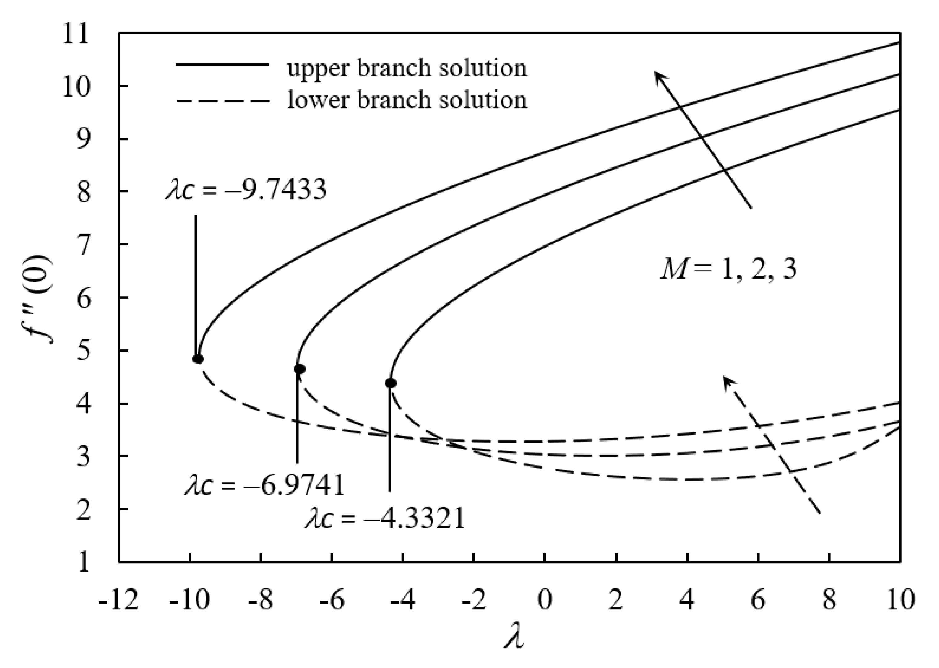
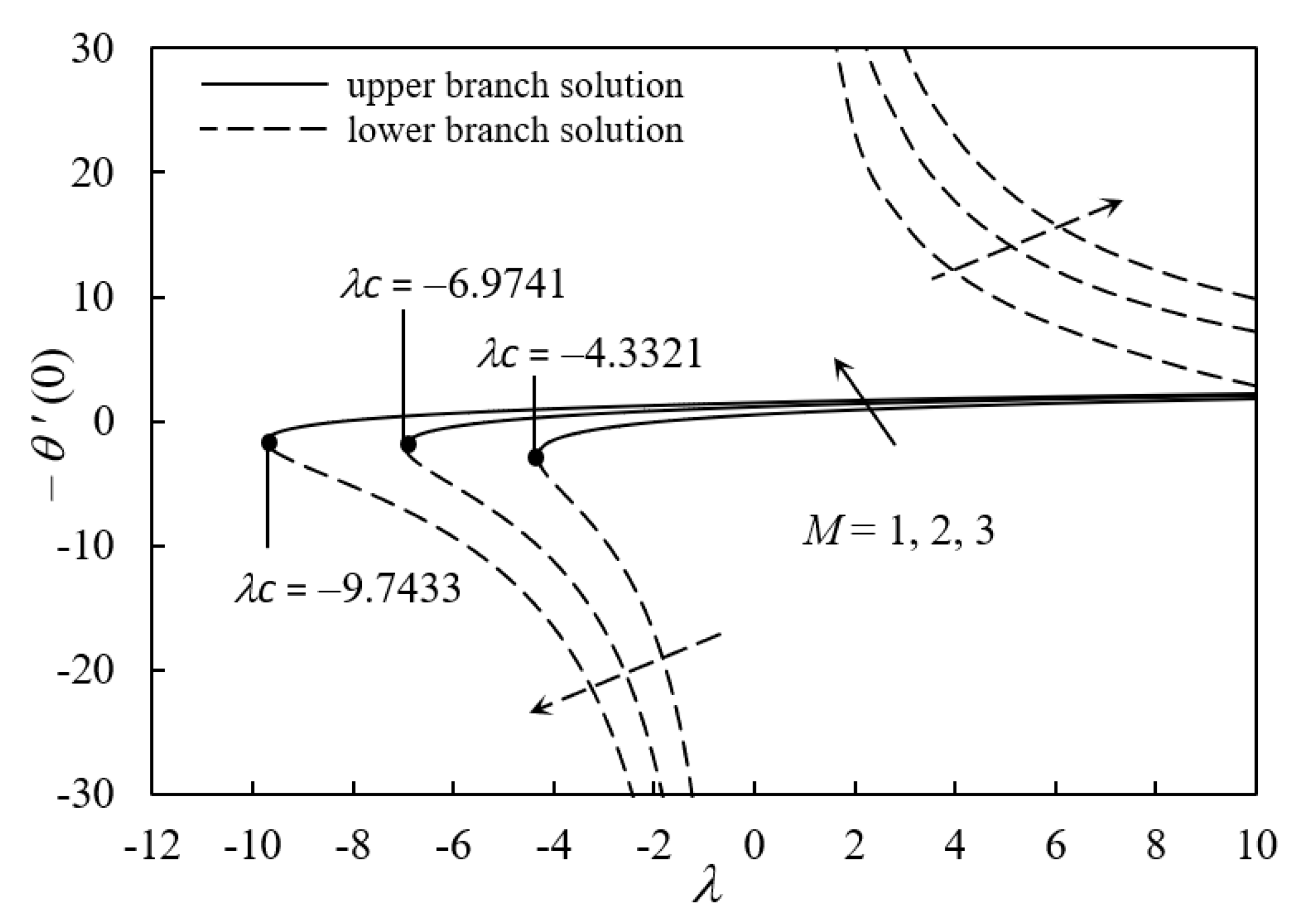
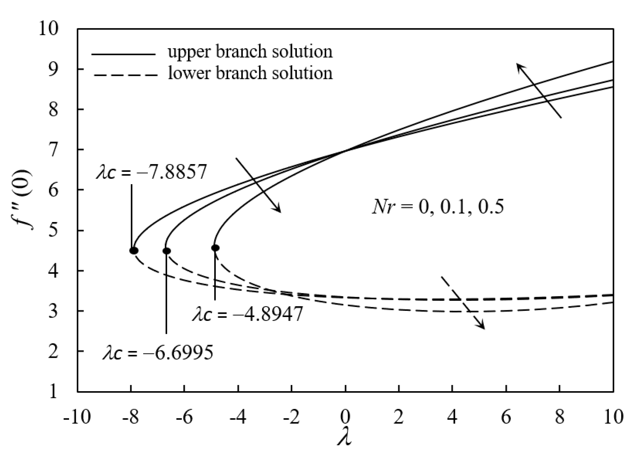
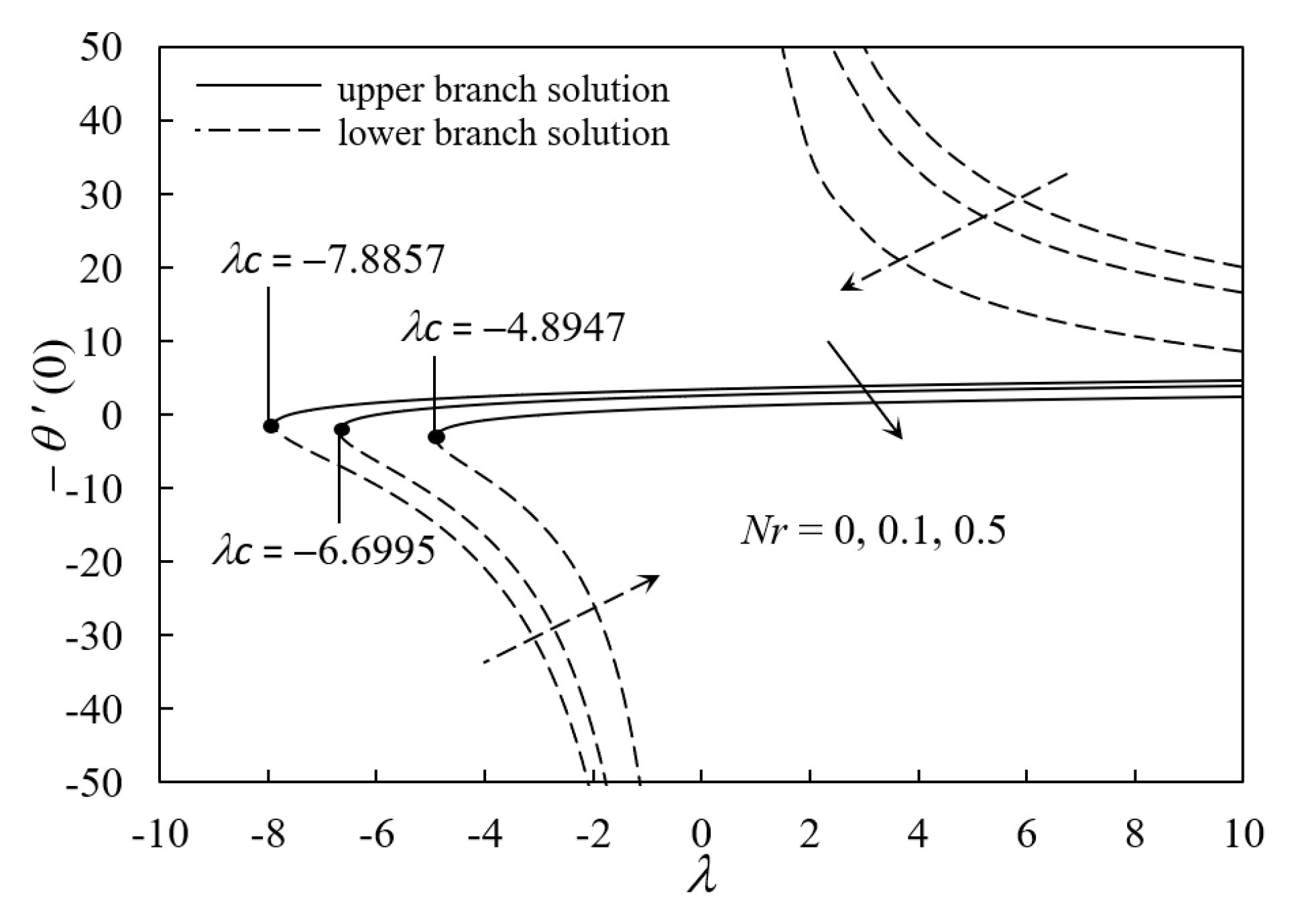
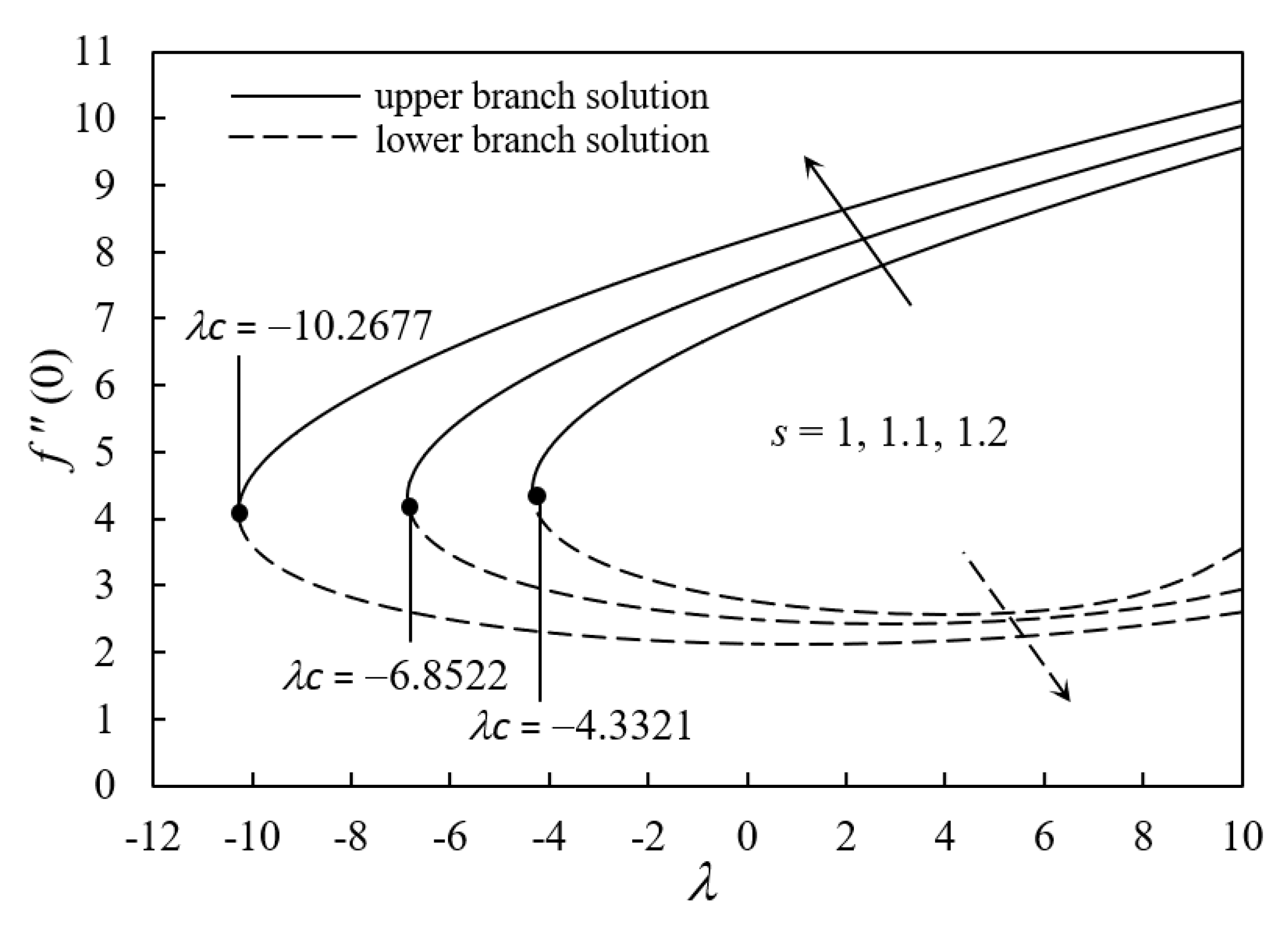
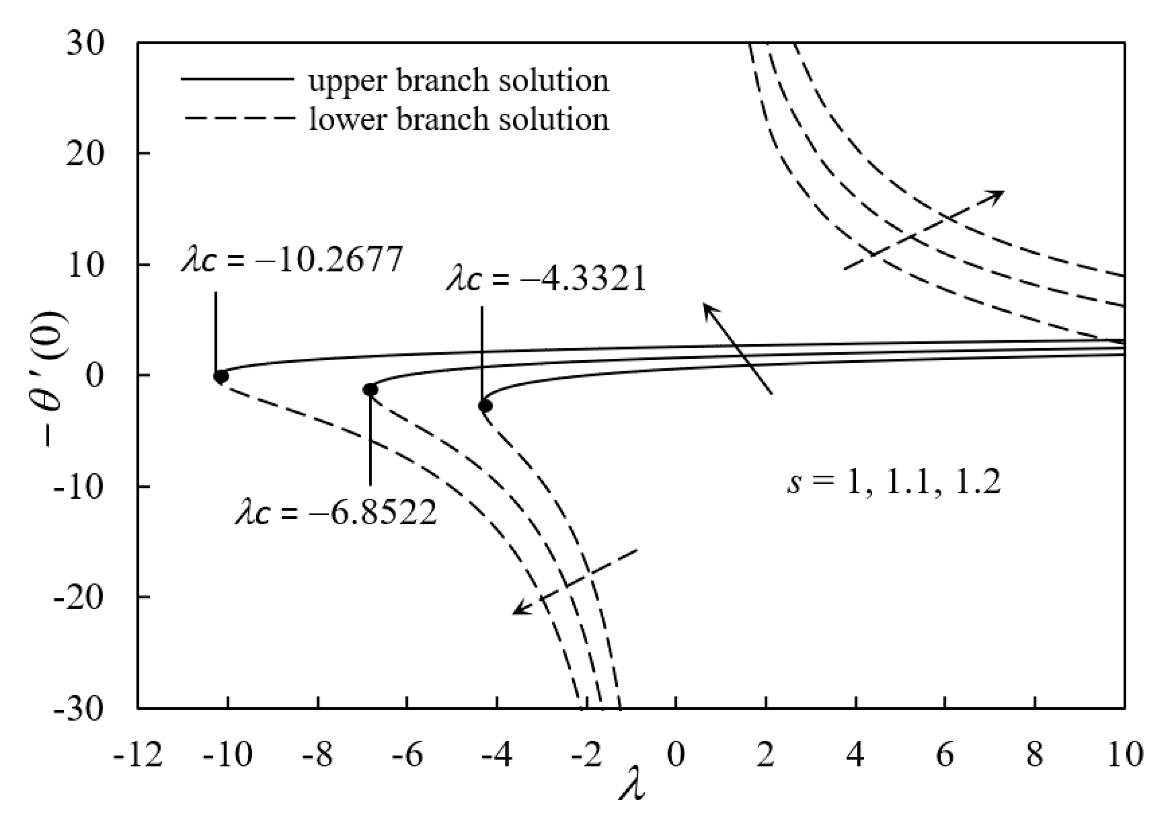
• The existence and duality of solutions were clearly demonstrated for the opposing flow and assisting flow.
• The solutions failed to exist for values of λ lower than the specified critical value for the opposing flow region.
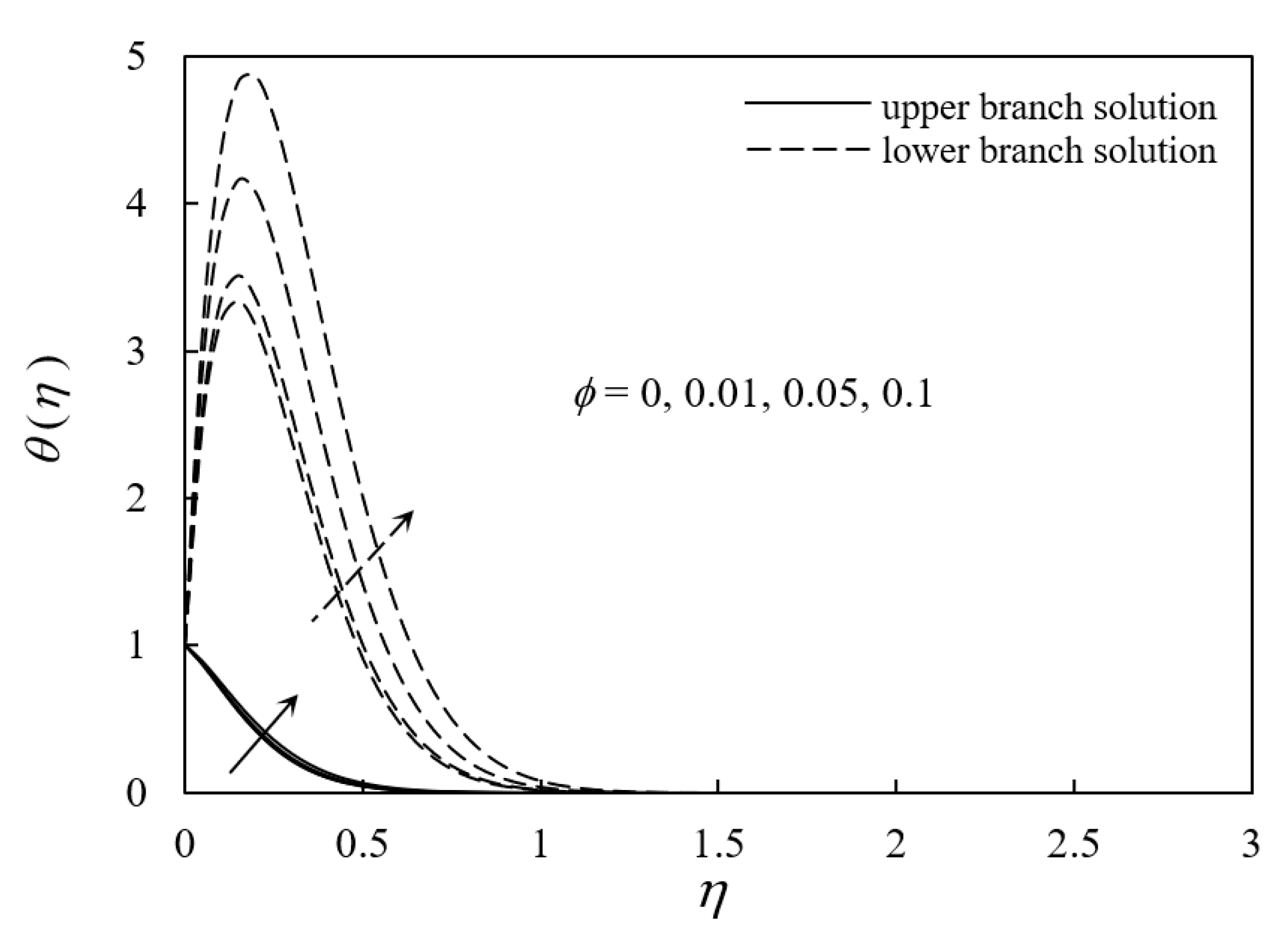
• The stability of the dual solutions validated that the upper branch solution was stable while it was unstable for the lower branch solution.
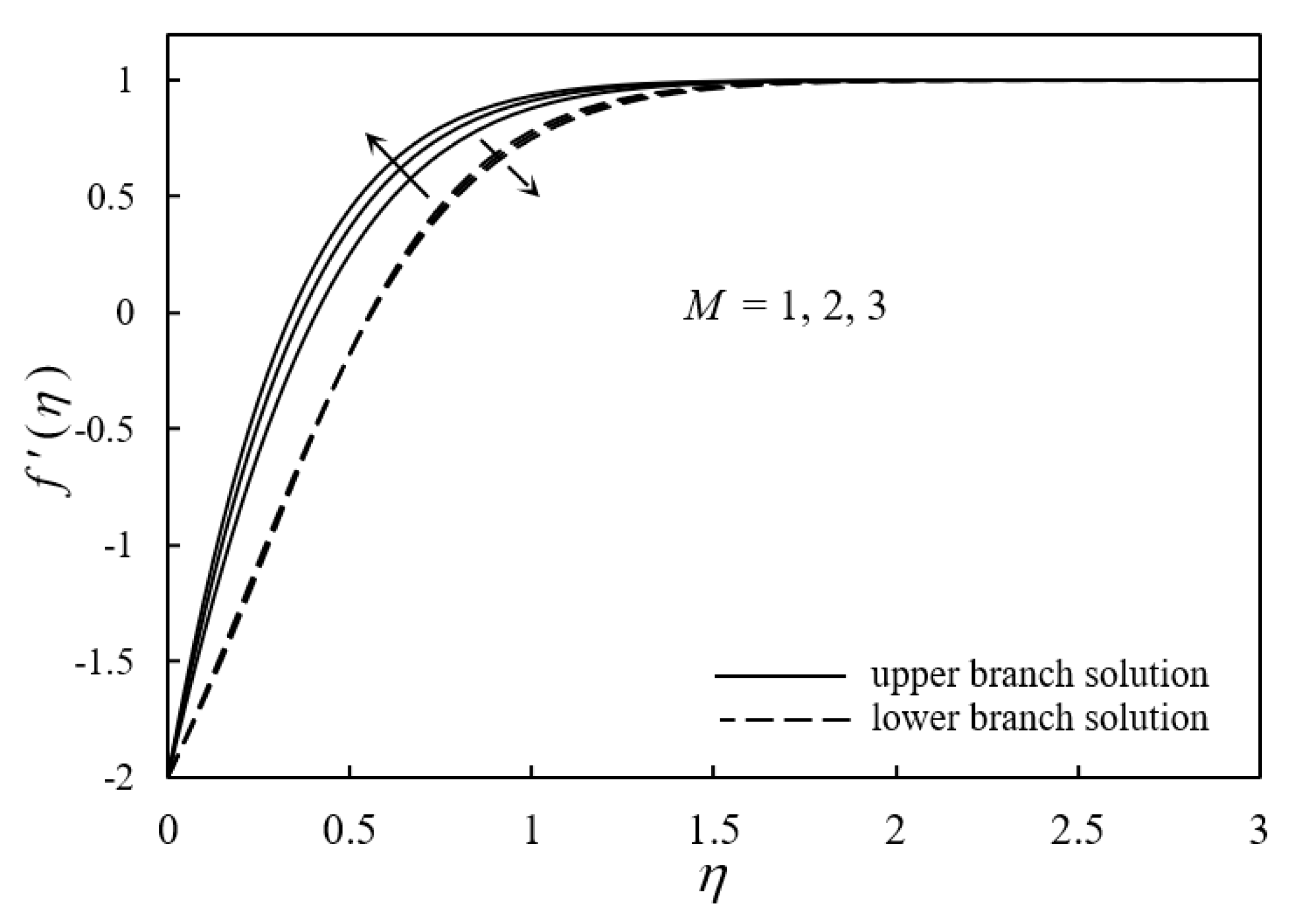
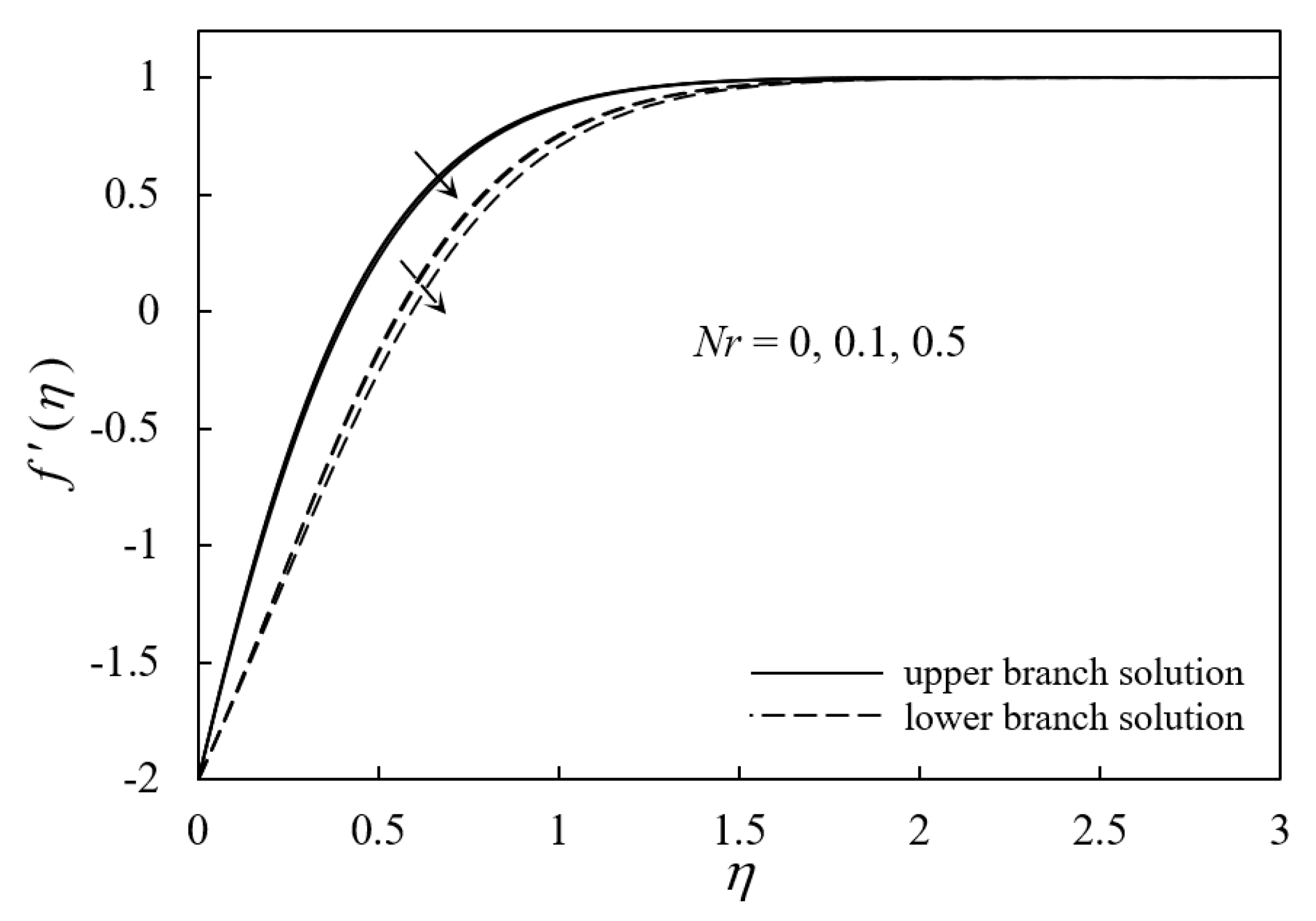
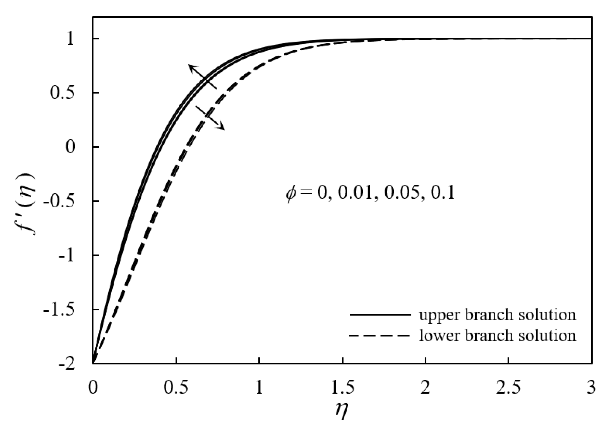
• Ferrofluid velocity profiles increased with an increase in M and ϕ but decreased with an increment in Nr.
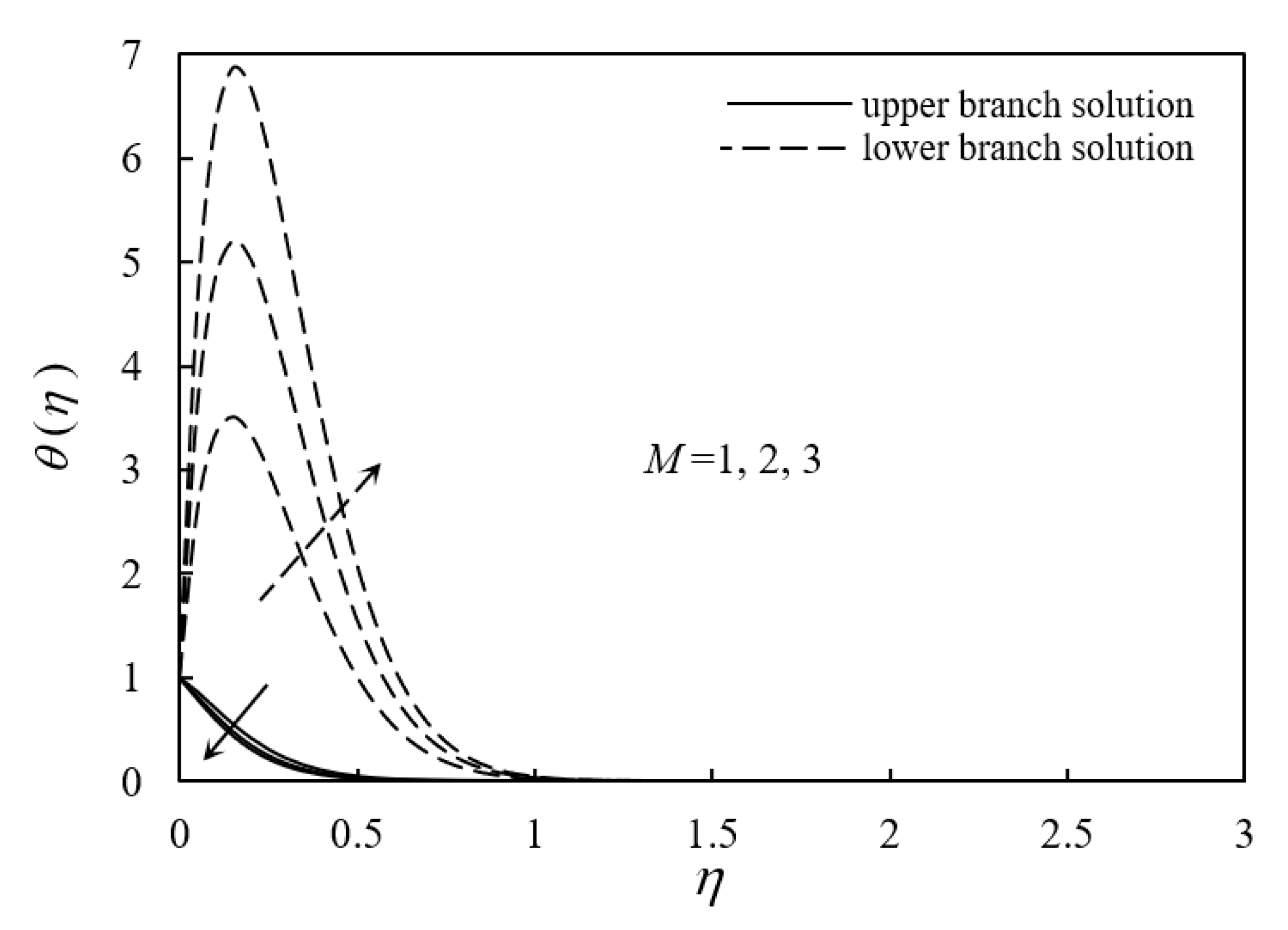
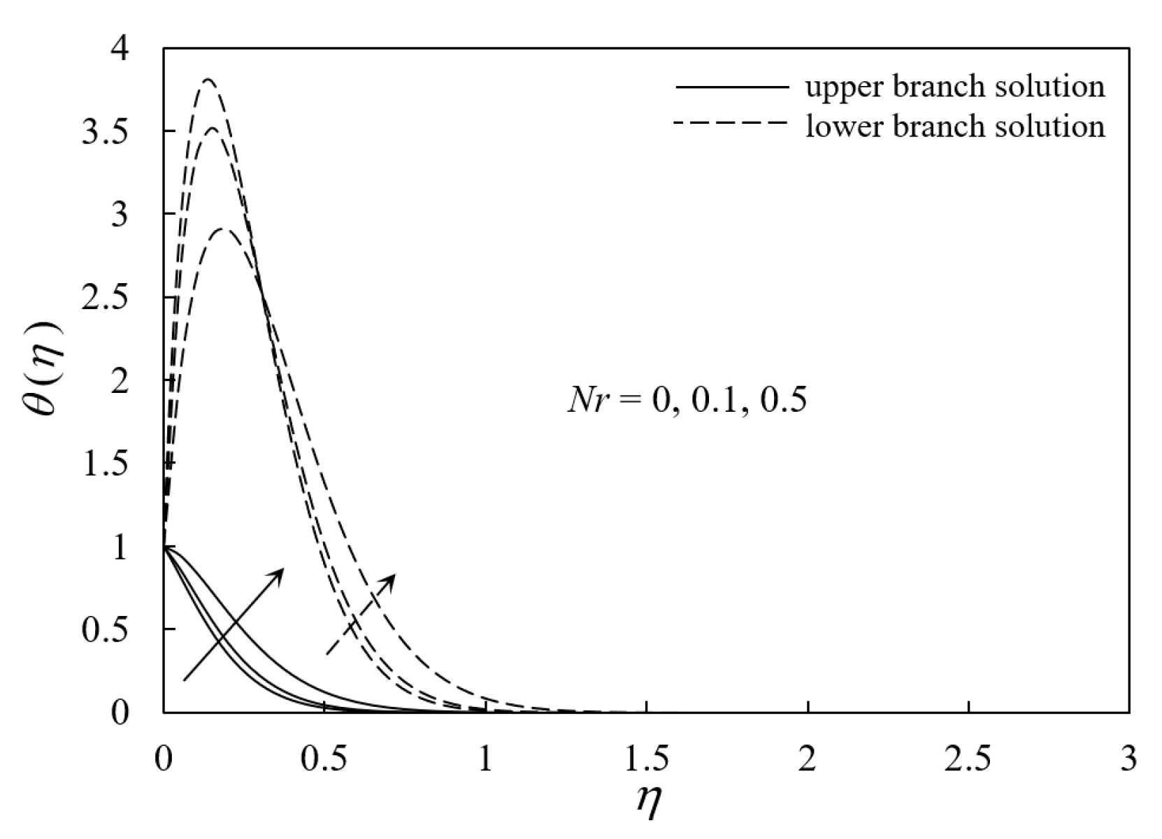
• Temperature profiles of the ferrofluid decreased with an increase in M; however, they increased with increasing ϕ and Nr.

References

1. Choi, S.U.S.; Eastman, J.A. Enhancing thermal conductivity of fluids with nanoparticles. ASME Publ. Fed. 1995, 231, 99–106. [Google Scholar]
2. Saidur, R.; Leong, K.Y.; Mohammad, H. A review on applications and challenges of nanofluids. Renew. Sustain. Energy Rev. 2011, 15, 1646–1668. [Google Scholar] [CrossRef]
3. Ahmad, S.; Pop, I. Mixed convection boundary layer flow from a vertical flat plate embedded in a porous medium filled with nanofluids. Int. Commun. Heat Mass Transf. 2010, 37, 987–991. [Google Scholar] [CrossRef]
4. Mahdy, A. Unsteady mixed convection boundary layer flow and heat transfer of nanofluids due to stretching sheet. Nucl. Eng. Des. 2012, 249, 248–255. [Google Scholar] [CrossRef]
5. Tamim, H.; Dinarvand, S.; Hosseini, R.; Pop, I. MHD mixed convection stagnation-point flow of a nanofluid over a vertical permeable surface: A comprehensive report of dual solutions. Heat Mass Transf. 2014, 50, 639–650. [Google Scholar] [CrossRef]
6. Mustafa, I.; Javed, T.; Majeed, A. Magnetohydrodynamic (MHD) mixed convection stagnation point flow of a nanofluid over a vertical plate with viscous dissipation. Can. J. Phys. 2015, 93, 1365–1374. [Google Scholar] [CrossRef]
7. Subhashini, S.V.; Sumathi, R.; Momoniat, E. Dual solutions of a mixed convection flow near the stagnation point region over an exponentially stretching/shrinking sheet in nanofluids. Meccanica 2014, 49, 2467–2478. [Google Scholar] [CrossRef]
8. Ibrahim, W.; Shankar, B. MHD boundary layer flow and heat transfer of a nanofluid past a permeable stretching sheet with velocity, thermal and solutal slip boundary conditions. Comput. Fluids 2013, 75, 1–10. [Google Scholar] [CrossRef]
9. Yazdi, M.; Moradi, A.; Dinarvand, S. MHD mixed convection stagnation-point flow over a stretching vertical plate in porous medium filled with a nanofluid in the presence of thermal radiation. Arab. J. Sci. Eng. 2014, 39, 2251–2261. [Google Scholar] [CrossRef]
10. Pal, D.; Mandal, G. Influence of thermal radiation on mixed convection heat and mass transfer stagnation-point flow in nanofluids over stretching/shrinking sheet in a porous medium with chemical reaction. Nucl. Eng. Des. 2014, 273, 644–652. [Google Scholar] [CrossRef]
11. Pal, D.; Mandal, G. Mixed convection–radiation on stagnation-point flow of nanofluids over a stretching/shrinking sheet in a porous medium with heat generation and viscous dissipation. J. Pet. Sci. Eng. 2015, 126, 16–25. [Google Scholar] [CrossRef]
12. Haroun, N.A.; Mondal, S.; Sibanda, P. Effects of thermal radiation on mixed convection in a MHD nanofluid flow over a stretching sheet using a spectral relaxation method. Int. J. Math. Comput. Phys. Electr. Comput. Eng. 2017, 11, 52–61. [Google Scholar]
13. Rosensweig, R.E. Magnetic fluids. Annu. Rev. Fluid Mech. 1987, 19, 437–463. [Google Scholar] [CrossRef]
14. Pîslaru-Dănescu, L.; Morega, A.M.; Morega, M.; Stoica, V.; Marinică, O.M.; Nouraş, F.; Păduraru, N.; Borbáth, I.; Borbáth, T. Prototyping a ferrofluid-cooled transformer. IEEE Trans. Ind. Appl. 2013, 49, 1289–1298. [Google Scholar] [CrossRef]
15. Bahiraei, M.; Hangi, M. Flow and heat transfer characteristics of magnetic nanofluids: A review. J. Magn. Magn. Mater. 2015, 374, 125–138. [Google Scholar] [CrossRef]
16. Çelik, Ö.; Can, M.M.; First, T. Size dependent heating ability of CoFe2O4 nanoparticles in AC magnetic field for magnetic nanofluid hyperthermia. J. Nanopart. Res. 2014, 16, 2321. [Google Scholar] [CrossRef]
17. Golneshan, A.A.; Lahonian, M. Diffusion of magnetic nanoparticles in a multi-site injection process within a biological tissue during magnetic fluid hyperthermia using lattice Boltzmann method. Mech. Res. Commun. 2011, 38, 425–430. [Google Scholar] [CrossRef]
18. Sharifi, I.; Shokrollahi, H.; Amiri, S. Ferrite-based magnetic nanofluids used in hyperthermia applications. J. Magn. Magn. Mater. 2012, 324, 903–915. [Google Scholar] [CrossRef]
19. Lajvardi, M.; Moghimi-Rad, J.; Hadi, I.; Gavili, A.; Isfahani, T.D.; Zabihi, F.; Sabbaghzadeh, J. Experimental investigation for enhanced ferrofluid heat transfer under magnetic field effect. J. Magn. Magn. Mater. 2010, 322, 3508–3513. [Google Scholar] [CrossRef]
20. Gavili, A.; Zabihi, F.; Isfahani, T.D.; Sabbaghzadeh, J. The thermal conductivity of water base ferrofluids under magnetic field. Exp. Therm. Fluid Sci. 2012, 41, 94–98. [Google Scholar] [CrossRef]
21. Khan, Z.H.; Khan, W.A.; Qasim, M.; Shah, I.A. MHD stagnation point ferrofluid flow and heat transfer toward a stretching sheet. IEEE Trans. Nanotechnol. 2014, 13, 35–40. [Google Scholar] [CrossRef]
22. Mustafa, I.; Javed, T.; Ghaffari, A. Heat transfer in MHD stagnation point flow of a ferrofluid over a stretchable rotating disk. J. Mol. Liq. 2016, 219, 526–532. [Google Scholar] [CrossRef]
23. Ilias, M.R.; Rawi, N.A.; Shafie, S. MHD Free Convection Flow and Heat Transfer of Ferrofluids over a Vertical Flat Plate with Aligned and Transverse Magnetic Field. Indian J. Sci. Technol. 2016, 9, 1–7. [Google Scholar]
24. Abbas, Z.; Sheikh, M. Numerical study of homogeneous–heterogeneous reactions on stagnation point flow of ferrofluid with non-linear slip condition. Chin. J. Chem. Eng. 2017, 25, 11–17. [Google Scholar] [CrossRef]
25. Reddy, J.R.; Sugunamma, V.; Sandeep, N. Effect of frictional heating on radiative ferrofluid flow over a slendering stretching sheet with aligned magnetic field. Eur. Phys. J. Plus 2017, 132, 7. [Google Scholar] [CrossRef]
26. Sivakumar, N.; Prasad, P.D.; Raju, C.S.; Varma, S.V.; Shehzad, S.A. Partial slip and dissipation on MHD radiative ferro-fluid over a non-linear permeable convectively heated stretching sheet. Results Phys. 2017, 7, 1940–1949. [Google Scholar] [CrossRef]
27. Shen, M.; Wang, F.; Chen, H. MHD mixed convection slip flow near a stagnation-point on a nonlinearly vertical stretching sheet. Bound. Value Probl. 2015, 2015, 78. [Google Scholar] [CrossRef] [Green Version]
28. Tiwari, R.K.; Das, M.K. Heat transfer augmentation in a two-sided lid-driven differentially heated square cavity utilizing nanofluids. Int. J. Heat Mass Transf. 2007, 50, 2002–2018. [Google Scholar] [CrossRef]
29. Jamaludin, A.; Nazar, R.; Pop, I. Three-dimensional magnetohydrodynamic mixed convection flow of nanofluids over a nonlinearly permeable stretching/shrinking sheet with velocity and thermal slip. Appl. Sci. 2018, 8, 1128. [Google Scholar] [CrossRef] [Green Version]
30. Hamid, R.A.; Nazar, R.; Pop, I. The non-alignment stagnation-point flow towards a permeable stretching/shrinking sheet in a nanofluid using Buongiorno’s model: A revised model. Z. Nat. A 2016, 71, 81–89. [Google Scholar] [CrossRef]
31. Bachok, N.; Najib, N.; Arifin, N.M.; Senu, N. Stability of dual solutions in boundary layer flow and heat transfer on a moving plate in a Copper-water nanofluid with slip effect. WSEAS Trans. Fluid Mech. 2016, 11, 151–158. [Google Scholar]
32. Roşca, N.C.; Pop, I. Axisymmetric rotational stagnation point flow impinging radially a permeable stretching/shrinking surface in a nanofluid using Tiwari and Das model. Sci. Rep. 2017, 7, 1–11. [Google Scholar] [CrossRef] [PubMed] [Green Version]
33. Pop, I.; Naganthran, K.; Nazar, R. Numerical solutions of non-alignment stagnation-point flow and heat transfer over a stretching/shrinking surface in a nanofluid. Int. J. Numer. Methods Heat Fluid Flow 2016, 6, 1747–1767. [Google Scholar] [CrossRef]
34. Naganthran, K.; Nazar, R.; Pop, I. Effects of heat generation/absorption in the Jeffery fluid past a permeable stretching/shrinking disc. J. Braz. Soc. Mech. Sci. Eng. 2019, 41, 1–12. [Google Scholar] [CrossRef]
35. Jamaludin, A.; Nazar, R.; Pop, I. Three-dimensional mixed convection stagnation-point flow over a permeable vertical stretching/shrinking surface with a velocity slip. Chin. J. Phys. 2017, 55, 1865–1882. [Google Scholar] [CrossRef]
36. Naganthran, K.; Nazar, R.; Pop, I. Stability analysis of impinging oblique stagnation-point flow over a permeable shrinking surface in a viscoelastic fluid. Int. J. Mech. Sci. 2017, 131–132, 663–671. [Google Scholar] [CrossRef]
37. Yatsyshin, P.; Kalliadasis, S. Coupled Mathematical Models for Physical and Biological Nanoscale Systems and Their Applications; Springer: Basel, Switzerland, 2018; pp. 171–185. [Google Scholar]
38. Lee, J.W.; Nilson, R.H.; Templeton, J.A.; Griffiths, S.K.; Kung, A.; Wong, B.M. Comparison of molecular dynamics with classical density functional and Poisson-Boltzmann theories of the electric double layer in nanochannels. J. Chem. Theory Comput. 2012, 8, 2012–2022. [Google Scholar] [CrossRef]
39. Garnett, J.M. Colours in metal glasses and in metallic films. Philos. Trans. R. Soc. 1904, 203, 385–420. [Google Scholar] [CrossRef]
40. Brinkman, H.C. The viscosity of concentrated suspensions and solutions. J. Chem. Phys. 1952, 20, 571–581. [Google Scholar] [CrossRef]
41. Merkin, J.H. On dual solutions occurring in mixed convection in a porous medium. J. Eng. Math. 1986, 20, 171–179. [Google Scholar] [CrossRef]
42. Weidman, P.D.; Kubitschek, D.G.; Davis, A.M. The effect of transpiration on self-similar boundary layer flow over moving surfaces. Int. J. Eng. Sci. 2006, 44, 730–737. [Google Scholar] [CrossRef]
43. Harris, S.D.; Ingham, D.B.; Pop, I. Mixed convection boundary-layer flow near the stagnation point on a vertical surface in a porous medium: Brinkman model with slip. Transp. Porous Med. 2009, 77, 267–285. [Google Scholar] [CrossRef]
44. Shampine, L.F.; Kierzenka, J.; Reichelt, M.W. Solving boundary value problems for ordinary differential equations in MATLAB with bvp4c. World J. Mech. 2013, 3, 4. [Google Scholar]
45. Shampine, L.F.; Gladwell, I.; Thompson, S. Solving ODEs with MATLAB; Cambridge University Press: New York, NY, USA, 2003; pp. 133–211. [Google Scholar]
46. Oztop, H.F.; Abu-Nada, E. Numerical study of natural convection in partially heated rectangular enclosures filled with nanofluids. Int. J. Heat Fluid Flow 2008, 29, 1326–1336. [Google Scholar] [CrossRef]
47. Babu, M.J.; Sandeep, N.; Raju, C.S.; Reddy, J.V.; Sugunamma, V. Nonlinear thermal radiation and induced magnetic field effects on stagnation-point flow of ferrofluids. J. Adv. Phys. 2015, 5, 1–7. [Google Scholar]
48. Nazar, R.; Jaradat, M.; Arifin, N.; Pop, I. Stagnation-point flow past a shrinking sheet in a nanofluid. Cent. Eur. J. Phys. 2011, 9, 1195–1202. [Google Scholar] [CrossRef]
Figure 1. Schematic diagram of the problem: (a) Stretching case, (b) shrinking case.
Processes 08 00095 g001
Figure 2. Variation of f ( 0 ) with λ for several values of M when Nr = 1, c = −2, and s = 1.
Processes 08 00095 g002
Figure 3. f ( η ) when Nr = 1, c = −2, s = 1, and λ = −2 as M varies.
Processes 08 00095 g003
Figure 4. Variation of θ ( 0 ) with λ for several values of M when Nr = 1, c = −2, and s = 1.
Processes 08 00095 g004
Figure 5. θ ( η ) for several values of M when Nr = 1, c = −2, s = 1, and λ = −2.
Processes 08 00095 g005
Figure 6. Variation of f ( 0 ) with λ for several values of Nr when M = 1, c = −2, and s = 1.
Processes 08 00095 g006
Figure 7. f ( η ) for several values of Nr when M = 1, c = −2, s = 1, and λ = −2.
Processes 08 00095 g007
Figure 8. Variation of θ ( 0 ) when M = 1, c = −2, and s = 1 as Nr varies.
Processes 08 00095 g008
Figure 9. θ ( η ) for several values of Nr when M = 1, c = −2, s = 1, and λ = −2.
Processes 08 00095 g009
Figure 10. The plots of f ( 0 ) with λ when M = 1, Nr = 1, and c = −2 as s varies.
Processes 08 00095 g010
Figure 11. The plots of θ ( 0 ) with λ when M = 1, Nr = 1, and c = −2 as s varies.
Processes 08 00095 g011
Figure 12. f ( η ) for several values of ϕ when M = 1, Nr = 0.1, c = −2, s = 1, and λ = −2.
Processes 08 00095 g012
Figure 13. θ ( η ) for several values of ϕ when M = 1, Nr = 0.1, c = −2, s = 1, and λ = −2.
Processes 08 00095 g013