Optimization Design and Analysis of Polymer High Efficiency Mixer in Offshore Oil Field

Abstract

The degree of polymer-water mixing in high-pressure pipelines on offshore oilfields usually influences the polymer solution’s performance. To realize efficient mixing of the polymer mother liquor with dilution water in the high-pressure pipeline, a high-efficiency mixer is designed and optimized. The designed mixer consists of four parts: a T-shaped pipe as the main body, an inlet flow-splitting plate, a stainless-steel flow-guiding tube, and an outlet flow-splitting plate. Mathematical models are built by using computational fluid dynamics (CFD) and the mixing effects are compared by using Fluent. The research results show that compared with conventional T-shaped mixers, the designed high-efficiency mixer has better mixing performance and increases the mixing rate to 80%. To optimize the mixing rate, the length of the stainless-steel tube is increased and the tube is perforated to guide the flow. The result shows that boring holes along straight lines around the tube can achieve good optimization effect and increase the mixing rate to 95%. The designed high-efficiency mixer can effectively improve the dissolving efficiency and solve problems in polymer-water mixing in the high-pressure pipeline.

1. Introduction

Polymer flooding technology has developed for many years in China, forming a complete set of polymer dissolution/injection process technology [1,2]. The most common polymer polyacrylamide for oil displacement can be dissolved by the triple dissolving device of dispersing dissolving tank, maturing tank, and static mixer [3,4,5]. However, due to the reservoir characteristics of loose sandstone and heavy oil in Suizhong 36-1 oilfield, it is difficult for polyacrylamide to effectively control the oil-water mobility [6,7,8]. With breakthroughs in the polymer-flooding technology on offshore oilfields, hydrophobic associated polymers that are suitable for ordinary offshore heavy oilfields have been designed [9,10,11]. The mechanism of hydrophobic association improves the property of the polymer solution but increases the difficulty in dissolving it in water [12,13]. This is because a small amount of hydrophobic groups on the macromolecular chain of hydrophobically associating polymer will block the entry of water molecules, thus prolonging the dissolution time of the polymer [14,15]. In the limited offshore platform space, it is difficult to fully mix and dissolve hydrophobically associating polymer under the polymer dissolving process device prepared in the land oilfield [16,17,18].

According to the quick dissolving mechanism of polymers, there are three measures to improve the mixing effect [19,20]. The first is increasing the polymer-water contact area to increase the area of exchange and hence improve mixing; the second measure is increasing the momentum of the polymers and water to increase the area of contact and mixing by mechanical power; another is increasing the temperature of the solution to accelerate mixing. Based on the accelerated dissolution mechanism of expanding contact area, a series of static mixers have been developed [21,22,23,24,25,26]. This is the most widely used method to accelerate the dissolution rate of polymer. Because the way of increasing momentum and temperature will be limited by actual conditions, for example, the way of equipment heating/insulation will greatly increase the application cost.

The polymer dissolution injection process of a platform in Suizhong 36-1 oilfield is taken as an example. Polymer dissolution is divided into two steps [27,28,29]: (1) the first step is to disperse and dissolve to prepare 5000 mg/L polymer solution, which is further dissolved in the maturing tank. The dissolution time of the whole process is 30 min, which can basically meet the initial dissolution conditions of this concentration of polymer; (2) the second step is to further dilute the polymer to 1750 mg/L, in which the polymer mother liquor is mixed with the dilution water in the high-pressure injection manifold. Before injection into the formation, it only takes 5 min to mix effectively, resulting in polymer/water two-phase after injection into the formation, which cannot reach the target solution performance required by polymer flooding.

At present, in the application platform of polymer flooding in offshore oil field, the poor mixed solution effect limits the expansion of application of polymer flooding, and effectively improves its mixed effect, which is the basis for further development and application of offshore oil field. Therefore, in order to improve the dissolution of hydrophobically associating polymer in offshore oil field. A high efficiency mixer was designed by computational fluid dynamics (CFD) software, and the mixing effect was compared. It provides technical support for the application and development of polymer flooding technology in offshore oil fields.

2. Design of High-Efficiency Mixer

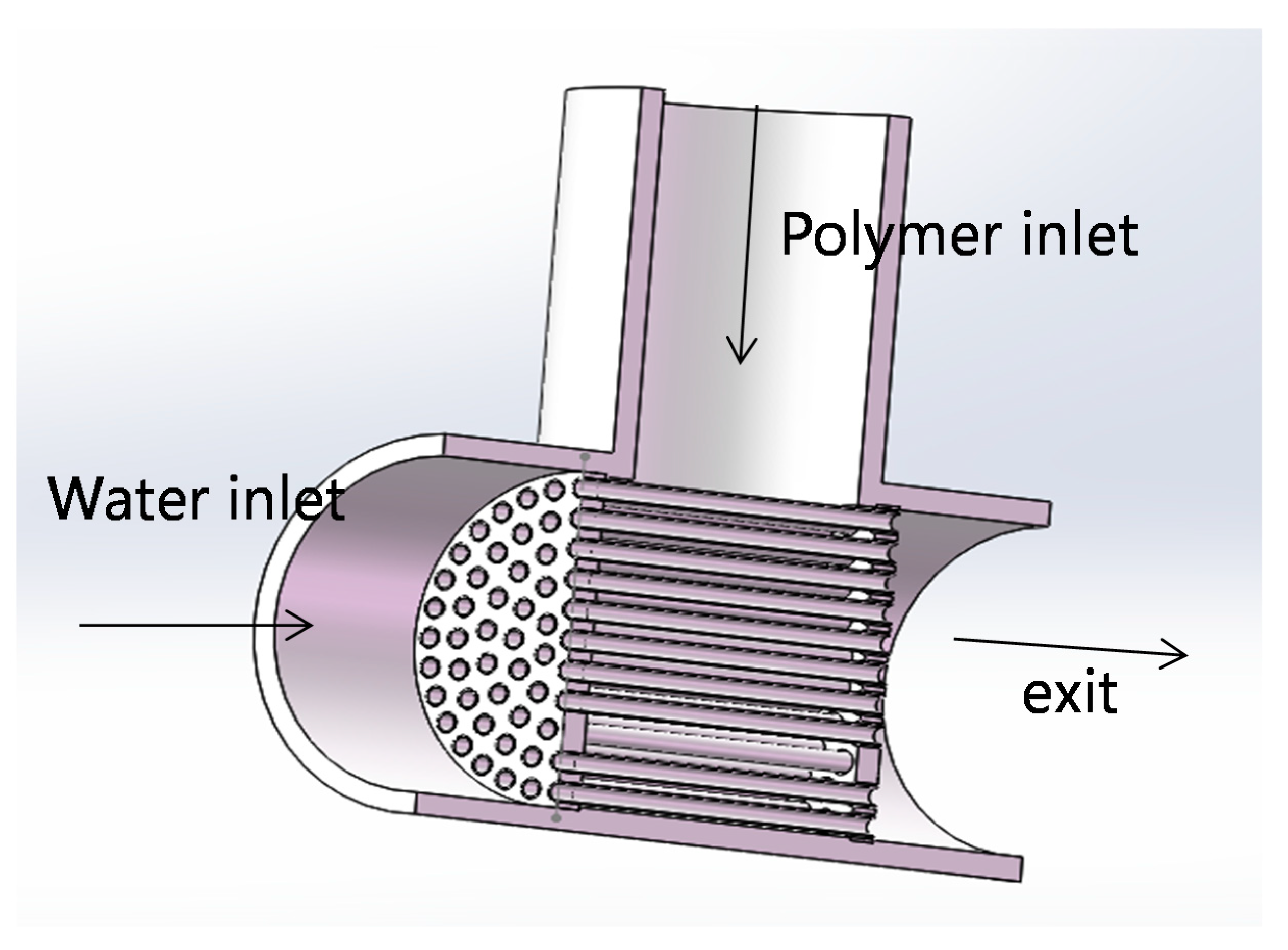
2.1. Design Idea

Due to the tough conditions offshore, it is not feasible to increase the solution’s temperature to accelerate mixing. The second measure is also not applicable because increasing the momentum of polymers and the water will not work well in the high-pressure environment. Thus, the first measure, increasing the contact area of the fluids, is the optimal choice. To increase the contact area, it is necessary to realize multi-channel mixing and take into account the influence of the shearing effect on the polymer solution. According to the working mechanism of multiport flow-splitting valves [30], we designed a high-efficiency mixer, as shown in Figure 1.

The high-efficiency mixer consists of four parts: a T-shaped pipe, an inlet flow-splitting plate, a stainless-steel flow-guiding tube, and an outlet flow-splitting plate. The T-shaped pipe is the main body of the mixer and is used to connect the polymer injection tube with the water injection tube. The inlet flow-splitting plate and the stainless-steel flow-guiding tube are fixed. The water is injected into the stainless-steel tube, and the polymers are filled around the tube.

According to the results of laboratory experiments, see

Table 1. The results of laboratory experiments.

Experimental Condition	Caliber Size mm	Viscosity of Polymer Solution mPa·s
Using formation water (total mineralization is 9300 mg/L [31,32]) from SZ36-1 oilfield in Bohai Sea to prepare polymer solution AP-P4 with concentration of 1750 mg/L [33]. The apparent viscosity of the solution was measured after passing through different sizes of pipe diameter at the injection rate of 10 mL/min.	20	161.25
	10	159.35
	8	157.21
	7	155.33
	6	124.71
	5	95.98
	4	47.32
	3	24.64
	2	15.32
	1	9.683

: when the diameter of copper pipe is less than 7 mm, the polymer solution with concentration of 1750 mg/L will be subject to strong mechanical degradation, and the apparent viscosity will be greatly reduced.

The outlet flow-splitting plate which has a larger diameter than that of the inlet flow-splitting plate is where the polymer solution and the water meet. The smaller the diameter of the copper tube, the stronger the shearing effect on the polymer solution. By physical experiments [34,35], we identified that when the inner diameter of the copper tube was 5.8 mm, the influence on the polymer’s shearing viscosity would be minimized, so we designed an 86-hole copper flow-guiding tube model.

The inner diameter of the tube is 115 mm, and the inlet on the left is a flow-splitting plate with thickness of 10 mm and an inner diameter of 7 mm. The plate is used to keep the 92 evenly-distributed flow-guiding copper tubes (130 mm long and with an inner diameter of 5.8 mm) fixed. The outlet flow-splitting plate connected to the tube on the right has an inner diameter of 8.6 mm and thickness of 10 mm.

2.2. Numerical Modeling and Parameters

The finite volume method is used for spatial discretization, and the coupling solver is used to solve the control equations [36]. Presto discretization is used for pressure spatial discretization, and the relatively steady first-order upwind scheme is used for the momentum equation, mass-conservation equation and the turbulence equation. The two phases are the polymer and water.

(1)

Constant mass flow is adopted as the boundary condition at the entrance boundary. According to the actual situation of the current injection concentration and injection amount of the polymer in the mine, the injected flow of polymer solution when it meets water is set at 75 m³/D, and the viscosity of the polymer solution at 5000 mg/L is 4000 mPa·s, and the injected flow of dilution water is 325 m³/D, and the viscosity of the water solution is 1 mPa·s.

(2)

The outlet boundary condition is constant pressure boundary condition, and the pressure is standard atmospheric pressure.

(3)

The no-slip condition is considered as the solid wall boundary condition, and the viscous sublayer is processed by the standard wall function.

(4)

Relaxation parameters: this is the default relaxation factor, and the convergence precision is the double precision.

(5)

Calculation residual: the calculation residual is less than 10⁻³, and it mainly monitors whether the outlet volume fraction is balanced as the basis for the calculation to reach stability.

(6)

Grid independence: the grid independence is verified, finally, the grid number is 15 million.

(7)

Discretization schemes: discrete format adopts the default simple algorithm.

2.3. Physical and Mathematical Modeling

2.3.1. Physical Model

(1) Model plotting and mesh generation: according to Figure 1, Model drawing: in order to study the mixing effect of different positions through the high-efficiency mixer, the 0.6 m pipe column distance at the liquid outlet end is extended on the basis of Figure 1, as shown in Figure 2.

(2) Mesh generation: the structured grid division method is adopted, and the local grid of the current limiting structure is encrypted to ensure the accurate capture of the convection field. See Figure 3 for the grid encryption at the entrance. The mesh quality is shown in Figure 4.

The mesh quality detection function is called through quality check in meshing. Apply determinant judgment. Determinant check is to calculate the Jacobian determinant value of each hexahedron, and then standardize the matrix of the determinant to represent the deformation of the element. A value of 1 indicates an ideal hexahedral cube, while 0 indicates an anti-cube with a negative volume. The mesh mass is represented by the x-axis, with all cells between 0 and 1. If the value of a cell determinant is 0, the cube has one or more degenerate edges. The number of elements is represented by y-axis, and the scale range is from 0 to the height of column. In general, determinants with values above 0.4 are acceptable for most solvers. which shows that the mesh quality is higher than 0.4, with high precision, meeting the calculation requirements.

2.3.2. Mathematical Model

By using Fluent for calculation, we decided to use the mixture model and the standard K-ε model as the mathematical model [37,38,39,40].

(1) Equation (1) is the mass conservation equation during the mixing process in steady conditions:

$$\frac{\partial {\rho }_m}{\partial t}+\frac{\partial }{\partial x_j}\left({\rho }_m{u}_j\right)=0$$

(1)

According to the percentage of the fluid volume, Equation (2) is obtained:

$${\rho }_m={\rho }_p{\alpha }_p+{\rho }_w{\alpha }_w,$$

(2)

where u_j is the velocity, t is the time, ${\rho }_m$ is the density of the polymer/water mixture, ${\alpha }_p$ is the polymer phase, and ${\alpha }_w$ is the water phase.

(2) The momentum conservation equations are as shown in Equations (3) and (4):

$$\frac{\partial }{\partial t}\left({\rho }_m{u}_i\right)+\frac{\partial }{\partial x_j}\left({\rho }_m{u}_i{u}_j\right)=-\frac{\partial p}{\partial x_i}+{\rho }_m{g}_i+\frac{\partial {\tau }_{ij}}{\partial x_i}$$

(3)

$${\tau }_{ij}={\mu }_m\left(\frac{\partial u_i}{\partial x_j}+\frac{\partial u_j}{\partial x_i}-\frac{2}{3}{\delta }_{ij}\frac{\partial u_k}{\partial x_k}\right),$$

(4)

where ${\mu }_m$ is the dynamic coefficient of viscosity, and ${\tau }_{ij}$ is the shear stress.

(3) The turbulence model is a K-ε model, as shown in Equations (5) and (6):

$$\frac{\partial }{\partial t}\left({\rho }_{m}k\right)+\frac{\partial }{\partial x_i}\left({\rho }_{m}k{\mu }_i\right)=\frac{\partial }{\partial x_j}\left[\left({\mu }_m+\frac{{\mu }_t}{{\sigma }_k}\right)\frac{\partial k}{\partial x_j}\right]+G_k+G_b-{\rho }_m\epsilon -Y_M+S_k$$

(5)

$$\frac{\partial }{\partial t}\left({\rho }_m\epsilon \right)+\frac{\partial }{\partial x_i}\left({\rho }_m\epsilon {\mu }_i\right)=\frac{\partial }{\partial x_j}\left[\left({\mu }_m+\frac{{\mu }_t}{{\sigma }_{\epsilon }}\right)\frac{\partial \epsilon }{\partial x_j}\right]+C_{1\epsilon }\frac{\epsilon }{k}\left(G_k+C_{1\epsilon }{G}_b\right)-C_{2\epsilon }\rho \frac{{\epsilon }^2}{k}+S_{\epsilon }$$

(6)

G_k is the turbulence kinetic energy caused by the velocity gradient, and can be obtained by Equation (7):

$$G_k={\mu }_i\left(\frac{\partial {\mu }_i}{\partial x_j}+\frac{\partial {\mu }_j}{\partial x_i}\right)\frac{\partial {\mu }_i}{\partial x_j}$$

(7)

G_b is the turbulence kinetic energy caused by buoyancy, and can be obtained by Equation (8):

$$G_b=\beta g_i\frac{{\mu }_t}{{Pr}_t}\frac{\partial T}{\partial x_i}$$

(8)

(4) Calculation equation of volume fraction. The volume fraction equation of the polymer as shown in Equation (9):

$$\frac{\partial }{\partial t}\left({\alpha }_p{\rho }_p\right)+\nabla \left({\alpha }_p{\rho }_p{\mu }_i\right)=-\nabla \left({\alpha }_p{\rho }_p{\mu }_{ip}\right),$$

(9)

where ${\alpha }_p$ is Volume fraction of polymer phase, ${\mu }_{ip}$ is Polymer viscosity.

3. Results and Discussion

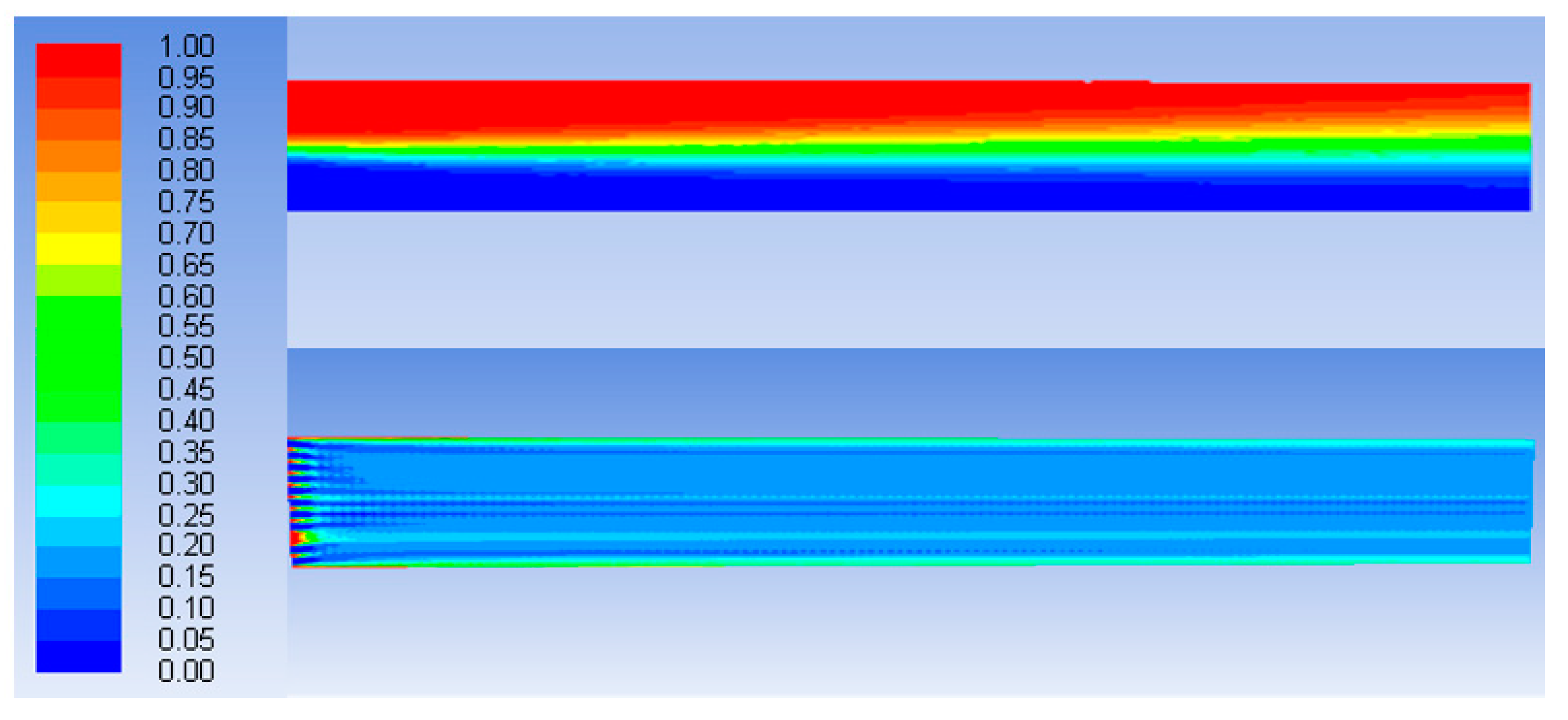
3.1. Mixing Effect of High-Efficiency Mixer

To compare the mixing effect of the designed high-efficiency mixer and that of common T-shaped pipes, we calculated the volume fraction of polymer at the X, Y, and Z sections in the designed mixer and in the ordinary T-shaped pipe. Red represents polymer solution with a volume fraction of polymer at 100%, blue represents the water solution with a volume fraction of water at 100%, and other colors in between represent other volume fractions [41]. Each number represents the percentage of water solution in the volume fraction of the mixture, for example, 0.9 means that the volume fraction of water is 10%, and the volume fraction of polymer is 90%.

(1) Mixing Effect at Section X

Figure 5 compares the volume fraction of polymer at the X section of the high-efficiency mixer and that of the ordinary T-shaped pipe. The upper part is the diagram of distribution of volume fractions of polymer in the ordinary T-shaped pipe, and the lower part shows the diagram of distribution of volume fractions of polymer in the high-efficiency mixer.

As Figure 5 shows, the polymer-water mixed solution in the ordinary T-shaped pipe was layered: polymers injected from the upper part of the pipe concentrated on the top and water concentrated at the bottom. As the flow moves forward, polymers and water were mixed and generated a transition region of green. In the simulated 0.6 m-long tube, the polymer solution could not be fully mixed with the water, and as the mixing distance grew, the high-viscosity polymer proceeded slowly, and the mixed polymer solution showed uneven densities, leading to a big difference in viscosity of the polymer solution injected to the bottom of the oil well. Compared with the ordinary T-shaped mixer, the high-efficiency mixer had better performance in mixing polymer with water, and a high mixing rate occurred at the outlet flow-splitting plate. In the simulated 0.6 m-long tube, the color is a mixed color of light blue and light green. Though the density of the mixture was uneven in some areas, it showed that the injected water has effectively diluted the polymer solution, and the mixing performance was far better than that in the ordinary T-shaped mixer.

(2) Mixing Characteristics at Y–Z Sections

Figure 6 shows comparison of the mixing effect at the Z section that is 0.01 m away from the outlets of two model mixers.

As Figure 6 shows, the polymer solution was obviously layered where it met the water. In the outlet section of the high-efficiency mixer, the water mixed with the polymer solution at the outlet after the flow of water was split into different columns by stainless-steel tubes, and each column of water was surrounded by high-viscosity polymer solution. The water-polymer contact area far exceeded that in the ordinary T-shaped pipe, so water and the polymer solution was more fully mixed and the mixing effect was improved.

(3) Distribution of Volume Fraction on X–Y Axis

The volume fraction of polymer at different locations of the Z axis in the high-efficiency mixer was compared. Three locations were selected for comparison: left (black dot line Z = 0.01 m), the middle location (green dot line Z = 0.4 m), and right (red dot line Z = 0.6 m).

As Figure 7 shows, the polymer solution at the inlet of the high-efficiency mixer concentrated on the pipe wall. This is because the polymer solution just met the water and had not been fully mixed. As the flowing distance grows, the polymer solution and water were evenly mixed. At the locations of 0.4 m and 0.6 m, the two curves show nearly the same trend on X axis and Y axis, which indicates that a good mixing effect was achieved. It also indicates that the polymer-water mixing effect was irrelevant to the manner of injection: whether it was water injection by copper tubes or polymer injection, the polymer solution and water showed characteristics of mixing at the middle section of the pipe.

3.2. Optimization of High-Efficiency Mixer

The high-efficiency mixer can improve the mixing effect, but the polymer-water mixing rate realized by the high-efficiency mixer only reached around 80%, and there is still room for improvement. Therefore, we optimized the mixer to further improve the mixing effect.

3.2.1. Design Idea and Model Optimization

The simulation tests above show that when the polymer mixed directly with water at the outlet flow-splitting plate, the contact area was (radius of outlet flow-splitting plate–radius of inlet flow-splitting plate)² × π × the number of copper tubes, as expressed by Equation (10).

$$S={\left(r_{out}-r_{in}\right)}^2\times \pi \times N$$

(10)

where S is the area of contact (m²), r_out is the radius of the outlet flow-splitting plate (m), r_in is the radius of the inlet flow-splitting plate (m), and N is the number of copper tubes.

Theoretically, to increase the mixing area can improve the mixing effect. There are different measures to increase the area of contact (as shown in Equation (5)), such as increasing the radius of the outlet flow-splitting plate, reducing the radius of the inlet flow-splitting plate or increasing the number of copper tubes. However, given the shearing effect, only by changing the flowing characteristics of the fluids and improving their interaction can the mixing effect be improved. The analysis above shows that the mixing effect did not show much difference whether the polymer went through the copper tubes or not, so the key to improving the mixing effect is to change the water’s flowing state and strengthen the flowing power in diluting the polymer solution.

As Figure 8 shows, we lengthened the copper tubes, extended the outlet flow-guiding plate, sealed and blocked the end of the tubes, bored holes of a fixed size around the tube so that the water would flow out of the tube along a direction perpendicular to the tubes rather than along the tubes. In this way, the water shot into the polymer solution and hence increased the momentum of mixing. We designed two schemes for hole-boring. Scheme A is to bore holes along straight lines, and a total of 16 holes are opened along the tube (4 holes on each of the four sides around the tube, and each side form an angle of 90° with the neighboring sides), with one hole at the end of the tube. Scheme B is to bore holes in a staggered way, and a total of 16 holes are bored (a total of 8 sides, each side forming an angle of 45° with neighboring sides, and 2 holes on each side, forming an angle of 90° with neighboring holes), with an extra hole bored at the end of the tube. To optimize the model, we increased the density of meshes around the holes and added a boundary layer to ensure stability of the flow.

3.2.2. Mixing Effect after Optimization

Figure 9 shows the simulation mixing result of Scheme A.

As Figure 9 shows, the mixing effect improved after the mixer was optimized. First, the X section showed an even distribution of the blue color, which was different from the effect before optimization. Despite uneven density of solution in a few areas at the front end of the pipe, most areas of the pipe showed evenly mixed density of solution. Second, at the cross section 0.02 m away from the outlet, the polymer solution no longer surrounded one single water column; instead, multiple water columns shot from the copper tubes mix with the polymer solution in a more thorough manner. Driven by the strong force of shooting, the water was shot into the polymer solution, which increased the momentum of contact between the polymer solution and water, and hence accelerated mixing. Third, according to the general effect analysis chart and the cross section 0.6 m away from the outlet, the optimized model improved the mixing effect and increased the mixing rate to 95%.

3.2.3. Influence of Different Pore-Opening Schemes

Figure 10 shows the simulation mixing result of Scheme B.

Figure 11 shows the effect of two different hole-boring schemes.

As Figure 11 shows, the color was evenly distributed and no layered phenomenon occurred when Scheme A is adopted. As the cross section 0.1 m away from the outlet shows, the color was evenly distributed, with only a few areas of light colors in the middle (the light color represents concentration of polymers), and there were more boundaries. The cross section 0.6 m from the outlet showed no difference in color, which means the solutions were fully mixed. When Scheme B was used, the X section 0.6 m from the outlet showed two noticeable layers, and at the section 0.1 m from the outlet, the polymer concentrated in the middle and forms a ring area of polymers. At the section 0.6 m from the outlet, the ring area still existed, but the difference in color reduced, which indicates a higher degree of mixing. The simulation result showed that Scheme A was better than Scheme B, and Scheme B resulted in heterogeneity of the mixed solution and worse mixing effect.

4. Conclusions

According to the actual needs of offshore oil field, the high-efficiency mixer is designed, which consists of four parts: a T-shaped pipe as the main body, an inlet flow-splitting plate, a stainless-steel flow-guiding tube, and an outlet flow-splitting plate. The mixing area of polymer solution and water is increased by diverting polymer/water. Research findings: First, the high-efficiency mixer that increases the polymer/water contact area can improve the polymers’ solubility when applied to offshore oilfields, and the mixing rate when the distance of contact is 0.6 m reaches 80%. Second, to improve the water flowing state at the outlet of the flow-guiding copper tube and bore four holes along straight lines with each side forming an angle of 90° with its neighboring sides, and add a hole at the end of the pipe can increase the mixing rate to 95%. In comparison, boring staggered holes performs worse in optimizing the mixer.

References

1. James, J.S.; Bernd, L.; Nasser, A. Status of Polymer-Flooding Technology. J. Can. Pet. Technol. 2015, 54, 116–126. [Google Scholar]
2. Lyadova, N.A.; Raspopov, A.V.; Bondarenko, A.V.; Kovalevskiy, A.I.; Cherepanov, S.S.; Baldina, T.R. Perspective application of the polymer flooding technology in the Perm region oil deposits (Russian). Oil Ind. J. 2016, 2016, 94–96. [Google Scholar]
3. Lederer, C.; Altstadt, S.; Andriamonje, S.; Andrzejewski, J.; Audouin, L.; Barbagallo, M.; Bécares, V.; Becvár, F.; Belloni, F.; Berthier, B.; et al. Society of Petroleum Engineers—SPE EOR Conference at Oil and Gas West Asia 2012, OGWA—EOR: Building Towards Sustainable Growth. In Proceedings of the SPE EOR Conference at Oil and Gas West Asia 2012—EOR: Building towards Sustainable Growth, OGWA Muscat, Oman, 16–18 April 2012. [Google Scholar]
4. Fan, H.J. Process Evaluation of the Colloid Injection and Allocation for Polyacrylamide. Oil Gas Field Surf. Eng. 2019, 8, 105–107. [Google Scholar]
5. Demin, W.; Youlin, J.; Yan, W.; Xiaohong, G.; Gang, W. Viscous-elastic polymer fluids rheology and its effect upon production equipment. SPE Prod. Facil. 2005, 19, 209–216. [Google Scholar] [CrossRef]
6. Jiang, W.C.; Zhang, J.; Song, K.P.; Tang, E.G.; Huang, B. Study on the Surfactant/Polymer Combination Flooding Relative Permeability Curves in Offshore Heavy Oil Reservoirs. Adv. Mater. Res. 2014, 53, 887–888. [Google Scholar] [CrossRef]
7. Jiang, H.; Chen, F.; Li, Y.; Zheng, W.; Sun, L. A Novel Model to Evaluate the Effectiveness of Polymer Flooding in Offshore Oilfield. In Proceedings of the Offshore Technology Conference-Asia, Kuala Lumpur, Malaysia, 25–28 March 2015. [Google Scholar]
8. Pi, Y.F.; Liu, J.J.; Xu, S.U. A Study of the Displacement Efficiency and Swept Efficiency to Enhance Oil Recovery. Int. J. Simul. Syst. Sci. Technol. 2016, 17, 19.1–19.6. [Google Scholar]
9. Zhang, C.; Ye, Z.B.; Shi, L.T.; Zhao, W.S.; Zhang, Z. A study on the mechanism to build flow resistance by hydrophobic associated polymer. China Offshore Oil Gas 2007, 19, 251–253. [Google Scholar]
10. Xie, K.; Cao, B.; Lu, X.; Jiang, W.; Zhang, Y.; Li, Q.; Song, K.; Liu, J.; Wang, W.; Lv, J.; et al. Matching between the diameter of the aggregates of hydrophobically associating polymers and reservoir pore-throat size during polymer flooding in an offshore oilfield. J. Pet. Sci. Eng. 2019, 177, 558–569. [Google Scholar] [CrossRef]
11. Xie, K.; Lu, X.; Li, Q.; Jiang, W.; Yu, Q. Analysis of Reservoir Applicability of Hydrophobically Associating Polymer. SPE J. 2016, 21, 1–9. [Google Scholar] [CrossRef]
12. Chen, H.; Wang, Z.M.; Ye, Z.B.; Han, L.J. The solution behavior of hydrophobically associating zwitterionic polymer in salt water. J. Appl. Polym. Sci. 2014, 131. [Google Scholar] [CrossRef]
13. Zhang, R.; Ye, Z.; Peng, L.; Qin, N.; Shu, Z.; Luo, P. The shearing effect on hydrophobically associative water-soluble polymer and partially hydrolyzed polyacrylamide passing through wellbore simulation device. J. Appl. Polym. Sci. 2013, 127, 682–685. [Google Scholar] [CrossRef]
14. Zhu, Y.J.; Zhang, J.; Zhao, W.S.; Wang, S.S.; Jing, B.; Meng, F.X.; Zhang, H. Research on Efficient Polymer Dissolving Technology for Hydrophobically Associating Polymer Flooding on Offshore Platform. In Proceedings of the 4th International Conference on Applied Mechanics, Materials and Manufacturing (ICAMMM), Shenzhen, China, 23–24 August 2014. [Google Scholar]
15. Xie, M.H.; Zhou, G.Z.; Liu, M.; Wu, H.; Long, X.L.; Yu, P.Q. Solubility of Hydrophobic Associating Polymer AP-P4 in Stirred Tank. J. East China Univ. Sci. Technol. (Nat. Sci. Ed.) 2010, 36, 323–333. [Google Scholar]
16. Chen, X. Screening and Evaluation of the Polymer Profile Control and Flooding System in Offshore Oil Field. Master’s Thesis, Northeast Petroleum University, Daqing, China, 2015. [Google Scholar]
17. Lu, Q. Study on the interaction between cyclodextrin and hydrophobically associating polymer. Master’s Thesis, Southwest Petroleum University, Chengdu, China, 2015. [Google Scholar]
18. Liu, L.W.; Zhang, J. Study on the Fast Dissolution of a Hydrophobic Association Water-Soluble Polymer. J. Southwest Pet. Univ. 2012, 3, 157–162. [Google Scholar]
19. Wang, Y.; Ye, Z.B.; Shu, Z.; Pu, J. A study on accelerating the solubility of hydrophobically associate polymer for offshore oilfield. Offshore Oil 2007, 2, 42–44. [Google Scholar]
20. Shi, Y. Study on Relationship between Solubility and Injection of New Polymer. Master’s Thesis, China Petroleum Exploration and Development Research Institute, Beijing, China, 2005. [Google Scholar]
21. Peter, G.M.K.; Shanmugasundaram, S. Polymer Melt Mixing in Static Mixers. In The Encyclopedia of Materials: Science and Technology; Elsevier: Amsterdam, The Netherlands, 2001; pp. 7428–7430. [Google Scholar]
22. Demoz, A. Scaling inline static mixers for flocculation of oil sand mature fine tailings. AIChE J. 2015, 61, 4402–4411. [Google Scholar] [CrossRef]
23. Liu, R.; Yuan, D.; Wang, Y.; Wang, J.; Jin, Y. Experimental study on a new tipe Static Mixer using in EOR injection polymer. Chem. Ind. Eng. Prog. 2011, 30, 475–478. [Google Scholar]
24. Newswire, P.R. Komax Hi-Pass Static Mixer Achieves More Than 25% Polymer Savings; PR Newswire: New York, NY, USA, 2018. [Google Scholar]
25. Ruphuy, G.; Weide, T.; Lopes, J.C.B.; Dias, M.M.; Barreiro, M.F. Preparation of nano-hydroxyapatite/chitosan aqueous dispersions: From lab scale to continuous production using an innovative static mixer. Carbohydr. Polym. 2018, 202, 20–28. [Google Scholar] [CrossRef] [Green Version]
26. Gholamali, F.; Elodie, B.; Timothy, F.L.M. Miniemulsions using static mixers: A feasibility study using simple in-line static mixers. J. Appl. Polym. Sci. 2009, 114, 3875–3881. [Google Scholar] [CrossRef]
27. Zhou, G.Z.; Xie, M.H.; Liu, M.; Wu, H.; Long, X.L.; Yu, P.Q. Dissolution Characteristics of Hydrophobically Associating Polyacrylamide in Stirred Tanks. Chin. J. Chem. Eng. 2010, 18, 170–174. [Google Scholar] [CrossRef]
28. Liu, M.; Zou, M.H.; Qiu, W.; Chao, S.Q.; Guo, P.W. High-efficient dissolution process design for polymer and its application in Bohai Oilfield. Pet. Eng. Constr. 2019, 45, 30–34. [Google Scholar]
29. Yu, Q.; Lu, X.G.; Zhang, D.F.; Xie, K. Accelerating Dissolution of Polyacrylamide in Offshore Oil Field. Bull. Korean Chem. Soc. 2015, 36, 2516–2520. [Google Scholar] [CrossRef]
30. Guo, G.F.; Ye, Z.B.; Shu, Z. Effects of Near Wellbore Shearing on the Seepage Characteristics of Flooding Polymer Solutions. Oilfield Chem. 2014, 1, 90–94. [Google Scholar]
31. Lederer, C.; Altstadt, S.; Andriamonje, S.; Andrzejewski, J.; Audouin, L.; Barbagallo, M.; Bécares, V.; Becvár, F.; Belloni, F.; Berthier, B.; et al. The effect of injection rate on recovery behaviors of hydrohobically water-soluble polymers after shearing. In Proceedings of the 16th International Conference on Fundamental Approaches to Software Engineering, FASE 2013, Held as Part of the European Joint Conferences on Theory and Practice of Software, ETAPS 2013, Rome, Italy, 16–24 March 2013. [Google Scholar]
32. Liu, Y.G.; Chen, H.X.; Tang, H.M.; Feng, Y.T.; Pang, M. Mechanism of scaling on reservoir formation damage by polymer-containing wastewater re-injection. Desalin. Water Treat. 2019, 139, 7–13. [Google Scholar] [CrossRef]
33. Guo, Y.; Hu, J.; Zhang, X.; Feng, R.; Li, H. Flow Behavior Through Porous Media and Microdisplacement Performances of Hydrophobically Modified Partially Hydrolyzed Polyacrylamide. SPE J. 2016, 21, 688–705. [Google Scholar] [CrossRef]
34. Ye, Z.B.; Wang, X.Y.; Shu, Z. Effect of shearing on the hydrodynamic radius distribution characteristics of polymer solution. Chem. Res. Appl. 2016, 28, 1268–1274. [Google Scholar]
35. Siregar, R.E.K.; Syam, B.; Wirjosentono, B.; Muttaqin, M. Static simulation to horse shoes alternative materials based basic polymeric foam reinforced fiberglass with ANSYS software. J. Phys. Conf. Ser. 2018, 1116, 42036. [Google Scholar] [CrossRef]
36. Wilcox, D.C. Reassessment of the scale-determing equation for advanced turbulence models. AIAA J. 1988, 26, 1299–1310. [Google Scholar] [CrossRef]
37. Pan, C.T.; Wang, S.Y.; Yen, C.K.; Ho, C.K.; Yen, J.F.; Chen, S.W.; Fu, F.R.; Lin, Y.T.; Lin, C.H.; Kumar, A.; et al. Study on Delamination Between Polymer Materials and Metals in IC Packaging Process. Polymers 2019, 11, 940. [Google Scholar] [CrossRef] [Green Version]
38. Cui, Z.D.; Liu, B.; Cai, J.; Huai, X.L. Analysis of simulation results for cavitating flows in micro-channels using different turbulence models. J. Univ. Chin. Acad. Sci. 2016, 33, 213–217. [Google Scholar]
39. Sahu, Y.K. Study on the Effective Thermal Conductivity of Fiber Reinforced Epoxy Composites. Master’s Thesis, National Institute of Technology, Rourkela, Odisha, India, 2014. [Google Scholar]
40. Murali, B.; Ramnath, B.V.; Chandramohan, D. Crash Test Analysis on Natural Fiber Composite Materials for Head Gear. Indian J. Sci. Technol. 2017, 10, 1–5. [Google Scholar] [CrossRef]
41. Malecha, Z.M.; Malecha, K. Numerical analysis of mixing under low and high frequency pulsations at serpentine micromixers. Chem. Process. Eng. 2014, 35, 369–385. [Google Scholar] [CrossRef]
Figure 1. The design diagram of the high efficiency mixer.
Processes 08 00110 g001
Figure 2. Physical model of high efficiency mixer.
Processes 08 00110 g002
Figure 3. Mesh generation.
Processes 08 00110 g003
Figure 4. Mesh quality analysis chart.
Processes 08 00110 g004
Figure 5. Comparison of mixing effects at the X section of two model mixers.
Processes 08 00110 g005
Figure 6. Mixing characteristics at Y–Z sections.
Processes 08 00110 g006
Figure 7. Distribution of volume fraction of polymer on different positions of X–Y axis.
Processes 08 00110 g007
Figure 8. Model of improved high-efficiency mixer.
Processes 08 00110 g008
Figure 9. Simulated mixing effect of the optimized mixer.
Processes 08 00110 g009aProcesses 08 00110 g009b
Figure 10. The simulation mixing result of Scheme B.
Processes 08 00110 g010
Figure 11. Mixing effect of different hole-boring schemes (Left is a; Right is b).
Processes 08 00110 g011