Numerical Simulation and Performance Prediction of Centrifugal Pump’s Full Flow Field Based on OpenFOAM

Abstract

The open-source software OpenFOAM 5.0 was used as a platform to perform steady-state and transient numerical simulation for full flow field of a pipeline centrifugal pump (specific speed n_s = 65) in a wide operating capacity range of 0.3Q_d~1.4Q_d. The standard k-ε and k-ω SST (Shear-Stress Transport) turbulence models were selected in the flow governing equations. The simpleFoam and pimpleDyMFoam solvers were used for the steady-state and transient calculations, respectively. ParaView, the postprocessor in OpenFOAM, was used to display the calculated flow velocity, pressure and streamline distributions, and to analyze the relationship between the vortex and the hydraulic loss in the pump. The external performance parameters of the pump such as head, input power and efficiency were also calculated based on the simulated flow fields. The predicted pump performances by OpenFOAM and Ansys-Fluent are compared with the test results under the same calculation model, grids and boundary conditions. The comparison indicates that OpenFOAM had high accuracy in the prediction of pump performance in the current case.

1. Introduction

Centrifugal pumps are widely applied in the processing industry, agricultural, civil and various other fields [1]. With the development of computational technology, the computational fluid dynamics (CFD) technique becomes very powerful and spans a wide range of industrial and non-industrial areas [2]. Commercial CFD software is convenient to use but the programming is usually unknown, so it is hard for users to modify or add models and algorithms according to their own ideas on certain issues. OpenFOAM, an object-oriented CFD open-source software, not only provides a wide range of standard solvers but also allows users to edit them in terms of the source code [3]. Due to the expandability and openness of source codes, recently some researches have been carried out on the flow field of pump machines by means of OpenFOAM. Petit et al. [4,5] and Nilsson [6], respectively, performed steady-state (frozen rotor method) and transient (sliding grid method) simulations on the flow field of centrifugal pumps and hydro turbines, and compared the results with the actual measurement. Xie [7] used 2D and 3D steady-state and transient methods to simulate the flow fields of a low specific speed centrifugal pump. Zhang [8] performed numerical calculations of turbulent flow for a high head turbine with k-ω SST (shear-stress transport) turbulence model and obtained the distribution of cavitating vapor in the turbine. Nuernberg and Tao [9] simulated the 3D tidal turbine array using a moving mesh with a rotor-stator interface to account for the effects of rotating tidal turbine blades and the flow field characteristics in tidal turbine arrays. Liu et al. [10] conducted a steady-state numerical simulation of the flow field in a centrifugal pump with specific speed n_s = 117.8 under three operating conditions (0.8Q_d, 1.0Q_d and 1.2Q_d) and found that the pump under the off-design operating conditions was well predicted by OpenFOAM 1.5-dev. However, due to the limitations of the solvers and post-processing functions of the previous OpenFOAM versions, the numerical results of the above-mentioned studies were far from satisfactory on the prediction accuracy of pump performance. Also, the researches based on OpenFOAM lacked in a full flow field of centrifugal pumps in a wide range of flow rates.

With the upgrade of the open source software OpenFOAM, the potential for computing pumps’ flow field and performance has significantly improved. In this work, therefore, a common pipeline centrifugal pump was selected by using OpenFOAM 5.0 to study the steady-state and transient full flow fields in a wide range (0.3Q_d~1.4Q_d) of operating conditions and to analyze the relationship between flow field and hydraulic loss in the pump with the updated post-processors. By comparing the measured results, the accuracy of OpenFOAM 5.0 software in predicting the performance of the centrifugal pump was analyzed.

2. Numerical Method and Model

2.1. Governing Equations

The governing equations of the fluid flow in this work included the continuity equation and the momentum equation. For turbulent flow, the k-ε model is used widely for internal flows, which provides an efficient method of calculating engineering flows [11]. Also, Liu et al. [10] found that the standard k-ε turbulence model had higher accuracy in computation of centrifugal pump performance after comparing with RNG (ReNormalization Group) k-ε and k-ω SST models. However, Shojaeefard et al. [12] found that the near-wall flow could be evaluated with high precision using the k-ω SST model, and the results had better accuracy than those of the k-ε model in a centrifugal pump simulation. Therefore, both the standard k-ε model and the k-ω SST model were chosen for the simulation in this study. All the governing equations can be expressed in a general differential formulation:

$$\frac{\partial }{\partial t}\left(\rho \varphi \right)+\frac{\partial }{\partial x_j}\left(\rho u_i\varphi \right)=\frac{\partial }{\partial x_j}\left(\Gamma \frac{\partial \varphi }{\partial x_j}\right)+S$$

(1)

where $\rho$ is the density of the fluid, $u_i$ is the i-directional component of the velocity vector, $\varphi$ is the arbitrary scalar, $\mathsf{\Gamma }$ is the diffusion coefficient, and S is the source term. The items in Equation (1) from left to right are transient items, convection items, diffusion items and source items. For different equations, $\varphi$, $\Gamma$ and $S$ have different forms.

Table 1. Specific forms of the symbols in Equation (1).

Equation	$\mathit{\varphi }$	$\mathsf{\Gamma }$	$\mathit{S}$
Continuity equation	1	0	0
Momentum equation	$u_i$	$\mu$	$-\frac{\partial p}{\partial x_i}+S_i$
Turbulent kinetic energy equation	k	$\mu +\frac{{\mu }_t}{{\sigma }_k}$	$G_k+S_k-\rho \epsilon$
Turbulence eddy dissipation equation	ε	$\mu +\frac{{\mu }_t}{{\sigma }_{\epsilon }}$	$C_{1\epsilon }\frac{\epsilon }{k}{G}_k-C_{2\epsilon }\rho \frac{{\epsilon }^2}{k}+S_{\epsilon }$

shows the detailed forms of the parameters $\varphi$, $\Gamma$ and $S$ for different equations, in which the turbulence model is the standard k-ε model.

In these equations, $\mu$ is dynamic viscosity. The turbulent viscosity ${\mu }_t$ is computed by combining k and ε as follows:

$${\mu }_t=\rho C_{\mu }\frac{k^2}{\epsilon }$$

(2)

$C_{\mu }$, $C_{1\epsilon }$, $C_{2\epsilon }$, ${\sigma }_k$ and ${\sigma }_{\epsilon }$ are model constants. $G_k$ represents the generation of turbulence kinetic energy due to the mean velocity gradients. $S_k$ and $S_{\epsilon }$ are source terms. $S_i$ is a generalized source term of the momentum conservation equation.

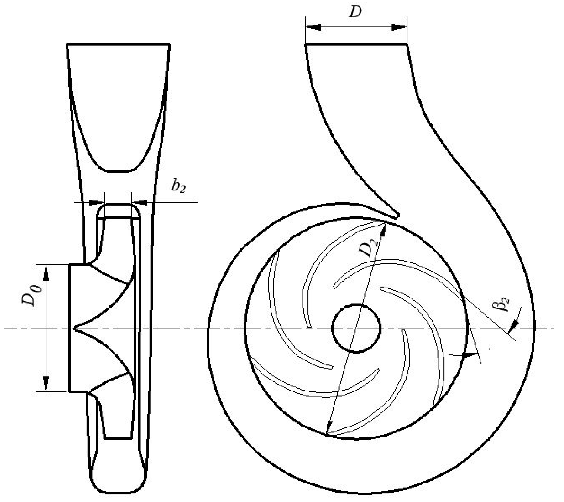
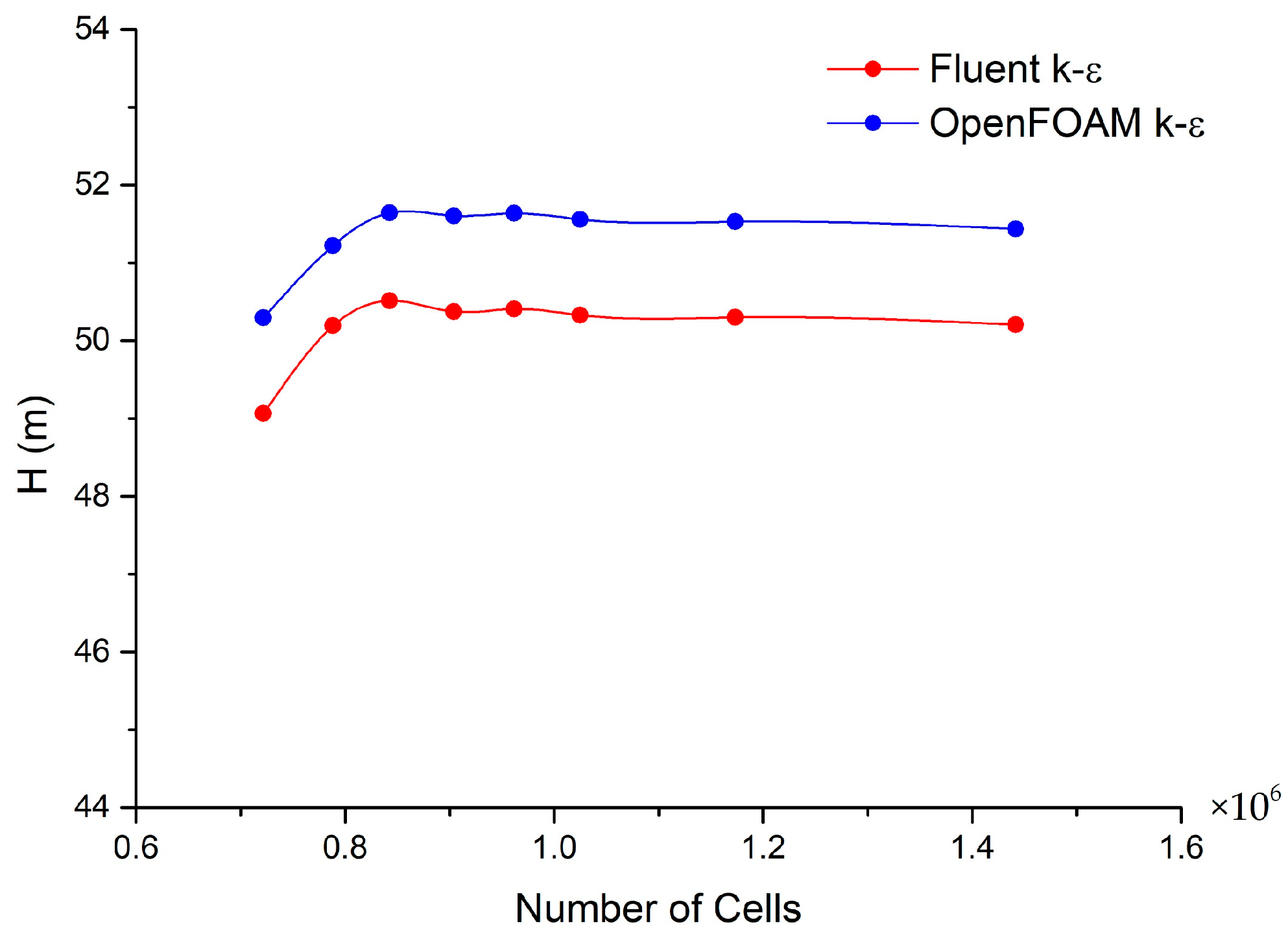
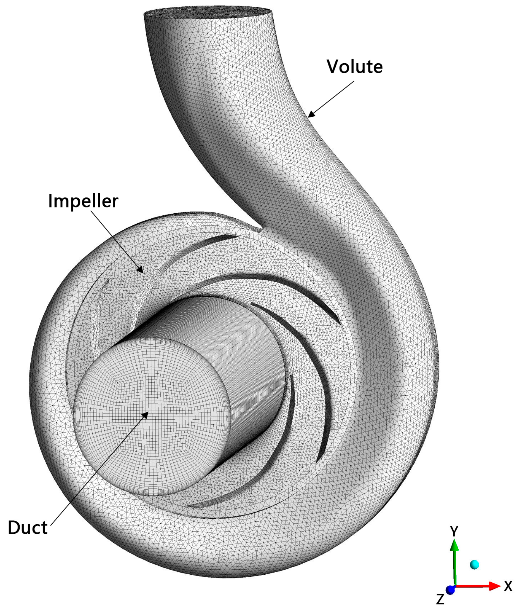
2.2. Computational Domain and Meshing

A common pipeline centrifugal pump of type IS125-100 was chosen for the research as shown in Figure 1. The design parameters for the centrifugal pump were: capacity (Q_d = 54 L/s), rotational speed (n = 2900 r/min), specific speed (n_s = 65), impeller inlet diameter (D₀ = 125 mm), impeller outlet diameter (D₂ = 216 mm), impeller outlet width (b₂ = 26.5 mm), impeller blade outlet angle (β₂ = 28°), number of impeller blades (Z = 6), discharge diameter (D = 100 mm). The computational domain was composed of an inlet pipe, impeller and volute. A 3D model was created by Pro-E software and imported into the ICEM software to generate the computational grid, which was converted into a format that OpenFOAM recognized. Since the domain of a centrifugal pump with such specific speed is complex, the grid is generally generated in an unstructured type for applications.

To choose a proper computational grid for simulation, the grid independency was examined. Figure 2 shows the relation between element number and calculated pump head with the standard k-ε turbulence model by Fluent and OpenFOAM. When the number of grids exceeded 1,000,000, the effect of the grids increase on the head was negligible, so the total number of elements in the simulation was 1,024,853 as shown in Figure 3.

2.3. Solvers and Boundary Conditions

The solver is the key tool for solving the discretization forms of the flow governing equations. The solvers, simpleFoam and pimpleDyMFoam, were used for the steady-state and transient simulations in this work, respectively. It was assumed that the pressure at the inlet of the pipeline pump was high enough and no cavitation occurred in the pump.

2.3.1. The SimpleFoam Solver

The simpleFoam is a steady-state incompressible flow solver in OpenFOAM, based on the SIMPLE (Semi-Implicit Method for Pressure Linked Equations) algorithm for pressure-velocity coupling [13]. In this algorithm, for a given pressure field (initial value or the result of the last iteration calculation), the discrete form of the flow governing equation is solved to obtain the velocity field for the next iteration. Under-relaxation factors ${\alpha }_u$ and ${\alpha }_p$ (${\alpha }_u+ {\alpha }_p=1$) were used to maintain iteration stability for velocity and pressure correction [14]. Also, the optimum convergence results with the combination of under-relaxation factors were found to be ${\alpha }_u=\left(0.7~0.8\right)$ and ${\alpha }_p=\left(0.3~0.2\right)$ [15]. Finally, the under-relaxation factors of velocity v, pressure p, turbulence kinetic energy k and turbulence dissipation rate ε or specific dissipation rate ω were 0.7, 0.3, 0.3, 0.3, respectively.

The “frozen rotor method” [16] was used in the simulations based on the multiple reference frame (MRF). The MRF approach implies that there is no relative mesh motion of the rotating and stationary parts. The solution of the steady-state, turbulent and incompressible flow of the impeller is governed by the Reynolds-averaged Navier-Stokes equations (RANS) in the rotating reference frame [4].

Arbitrary mesh interface (AMI) [17] was adopted to transfer the flux between the rotational impeller and stationary domain grids by a set of weighting factors both for steady-state and transient cases. The boundary conditions for the steady state computation were: (1) The type of velocity v, turbulent kinetic energy k and turbulent eddy dissipation ε or ω at the inlet were “fixedValue”. The value of v was given by the pump operation capacity, the initial values of k, ε and ω were calculated and the pressure type at the inlet was “zeroGradient”; (2) The pressure type at the outlet was “fixedValue”; (3) The no-slip solid wall condition was adopted in wall surfaces, and the standard wall function method was used to determine the flow around the solid wall. The turbulent parameters of wall functions, ${\mu }_t$, k, ε and ω were specified through the “nutkWallFunction”, “kqRWallFunction”, “epsilonWallFunction” and “omegaWallFunction” in terms of OpenFOAM code, respectively. Yplus (y+) is the dimensionless distance from the wall and is used to check the location of the first node. When standard wall functions are used, the value of y+ in the range 30~500 satisfies the log-law [18]. In the present study, thus, the values of y+ were set with the locations of the first nodes in the range of 30~300; (4) The type of the impeller wall was “movingwallVelocity”; (5) The impeller domain was defined by the “MRFProperties” file according to the “frozen rotor method”. For the discretizations, the second-order Gauss linear upwind convection schemes were adopted for a higher accuracy. For the gradient terms, the Gauss linear scheme was selected, and the residual criterion was set to 10⁻³.

2.3.2. The PimpleDyMFoam Solver

The pimpleDyMFoam solver, based on the PIMPLE (merged PISO (Pressure Implicit with Splitting of Operators)-SIMPLE) algorithm [19], is a reasonable time step transient for incompressible turbulent flow with dynamic meshes. The basic method in the PIMPLE algorithm is to use the PISO algorithm to step the time, and at each step the pressure field of a non-final iteration step and velocity field are solved. The solution of the time-dependent, turbulent and incompressible flow system of the pump is governed by the unsteady Reynolds-averaged Navier-Stokes equations (URANS) that can be in the formulations written for a moving control volume [20].

All boundary conditions for the transient case were consistent with those for the steady-state case except condition (5). The computational domain of the impeller was defined by the “dynamicMeshDict” file according to the “sliding mesh method” [21,22]. The first order implicit Euler scheme was adopted for the time discretization. The time step was set to be 5 × 10⁻⁵ s equivalent to the time for the impeller to rotate 1 degree, and the maximum Courant number was set to 5. The residual criterion was set to 10⁻⁶ and the maximum iterative loop was 100 in each time step.

3. Results and Analysis

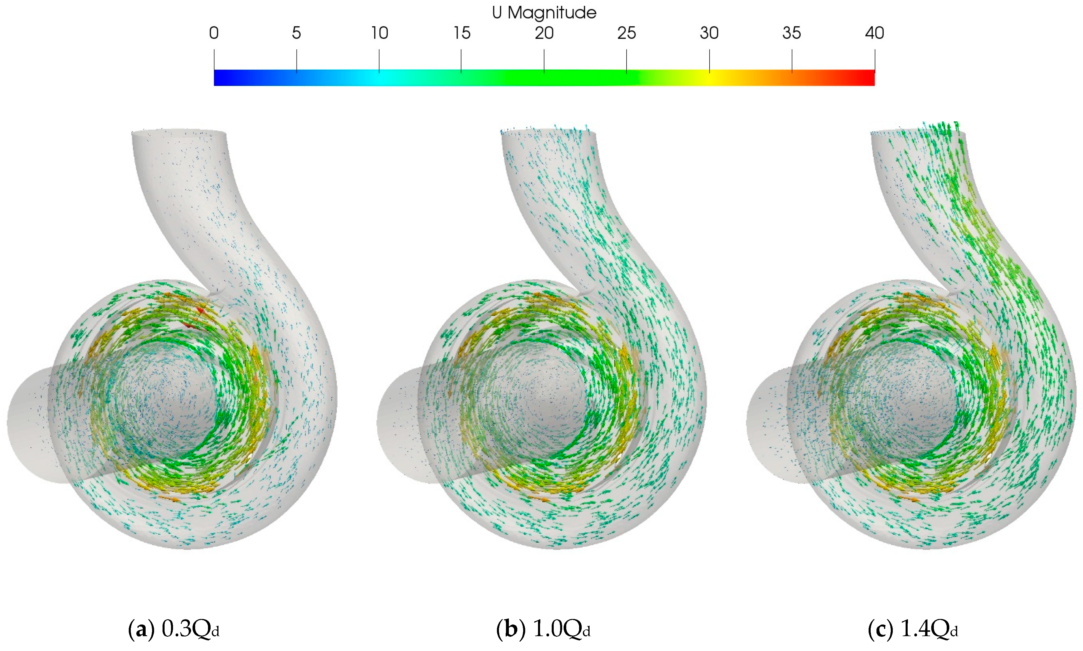
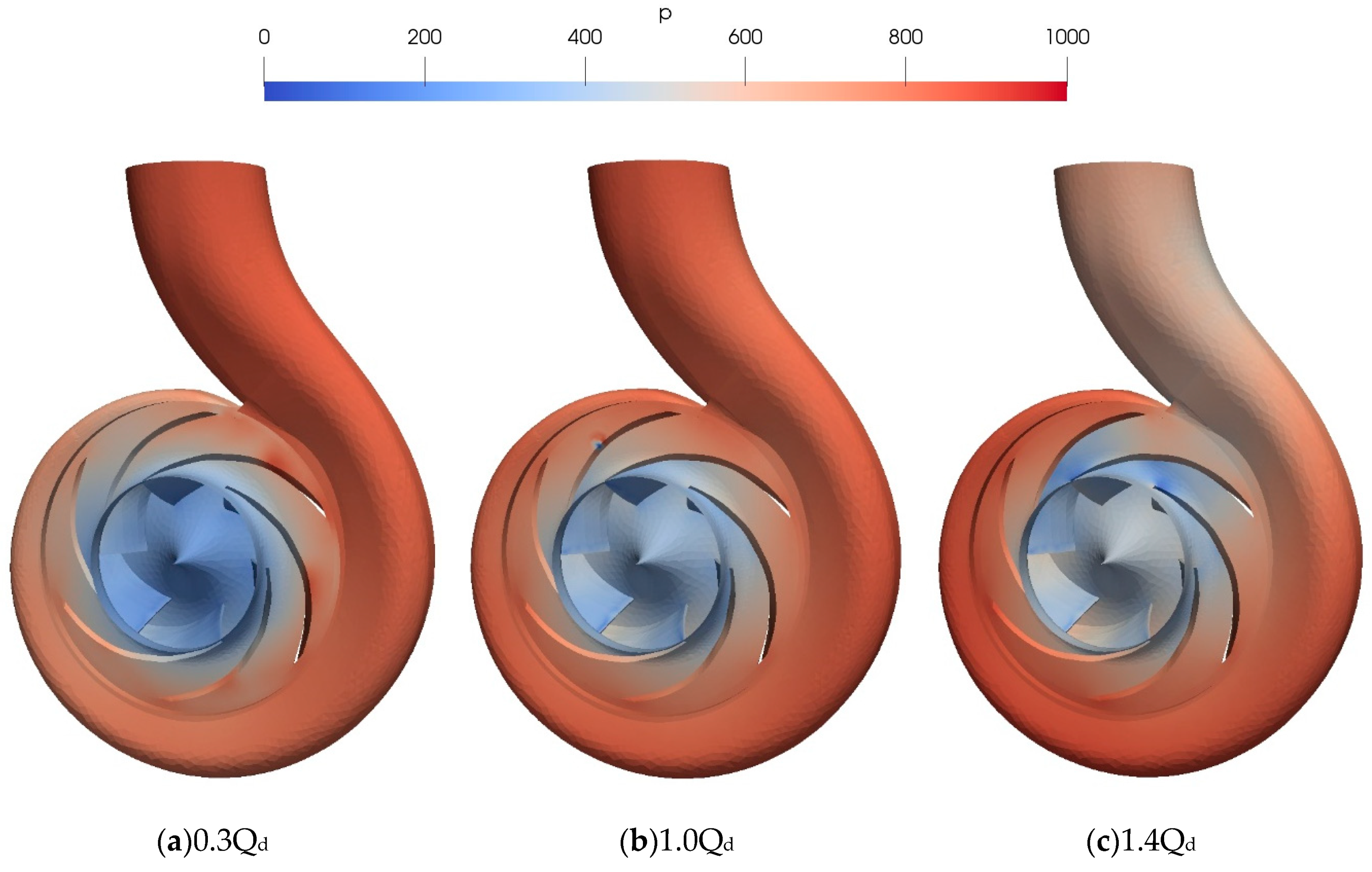
3.1. Pump Flow Field Distribution

The calculated results of flow fields can be displayed by ParaView (OpenFOAM’s postprocessor) or converted to other post-processing data formats. Figure 4 shows the flow velocity vectors in the pump by steady-state calculation under three operating conditions (0.3Q_d, 1.0Q_d and 1.4Q_d). It can be seen from the figure that due to the rotation of the impeller, the flow velocity in the impeller gradually increases along the radius, and the flow velocity at the impeller outlet reaches a maximum value. After entering the volute, the flow velocity decreases. Since the volute passage near the outlet is designed as a bend, the flow velocity outside the volute is higher than that inside near the outlet due to centrifugal force. Apparently, the velocity vectors in the volute appear too small or too large under the condition of 0.3Q_d or 1.4Q_d, indicating that the size of the volute is not suitable for these operating conditions.

Figure 5 and Figure 6 respectively show the distributions of the streamlines in the centrifugal pump projected on the central xy and zx planes (corresponding to Figure 3) by the steady-state calculation under three operating conditions. On the xy plane, under 0.3Q_d operating condition, the fluid passes the volute diffuser region in a lower velocity (Figure 5a). When the flow rate is 1.0Q_d, the main flow tends to follow the curvature of the volute outer wall (Figure 5b). Under the 1.4Q_d operating condition, a recirculation region is obviously observed on the inner wall near the volute exit due to a higher centrifugal force (Figure 5c). It is noted that flow velocity departing from the outlet of the impeller is more uniform (magnitude is about 20 m/s) under 1.0Q_d than at 0.3Q_d and 1.4Q_d operating conditions.

On the zx plane, there are some vortexes (see arrows in Figure 6) with different sizes in the inlet, impeller and volute under three operating conditions. Under the 0.3Q_d operating condition (Figure 6a), the inlet velocity is insufficient to overcome adverse pressure gradient and the separation flow phenomenon occurs at the duct, generating a couple of strong swirling vortexes in the separation point. In Figure 6, some vortexes are clearly observed in the volute cross sections, which belong to the secondary flow vortex which usually occurs in a bent pipe. In contrast, the vortexes under 1.0Q_d are less comparable to those under off-design conditions. These phenomena explain the reason that the hydraulic loss under off-design conditions is significant compared to that under the design condition.

Figure 7 shows the static pressure distribution per density of the fluid in the centrifugal pump by the steady-state calculations under the three operating conditions. It can be seen from the figure that the lowest static pressure zone is located around the leading edges of the impeller blades, while the highest pressure value appears at a certain position in the volute passage. From the point of view of fluid mechanics, hydraulic loss mainly includes friction loss and diffusion loss along the flow passage. Under the 0.3Q_d flow condition (Figure 7a), lower velocity in a larger size of volute leads to serious diffusion loss. Due to the increase of flow velocity under the high flow condition of 1.4Q_d (Figure 7c), the frictional loss increases and the static pressure also reduces at the outlet of the volute.

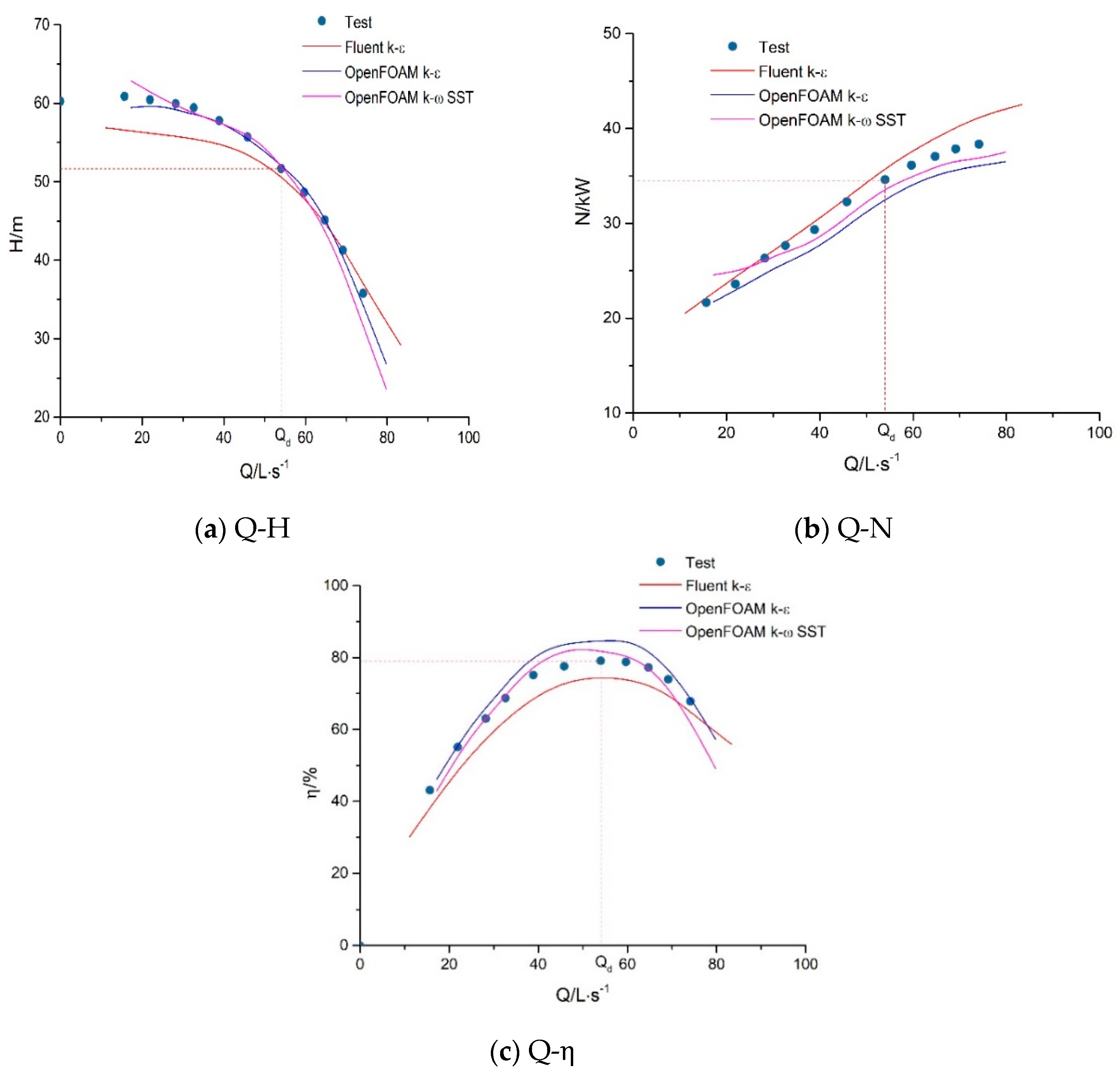
3.2. Pump Characteristics Prediction

Based on the numerical results of flow field in the pump, the external characteristic parameters such as head H, input power N and efficiency η can be calculated by Equations (3)~(5):

$$H=\frac{P_{out}-P_{in}}{\rho g}+h$$

(3)

$$N=M\omega$$

(4)

$$\mathsf{\eta }=\frac{\mathsf{\rho }\mathrm{gQH}}{\mathrm{N}}$$

(5)

where, $P_{out}$, $P_{in}$ is the average total pressure of the pump at outlet and inlet, respectively; h is the distance in gravity direction from the pump outlet to the inlet; $M$ is the torque acting on the inner flow surface of the impeller; $\omega =2\pi n/60$.

Figure 8 shows the steady-state and transient calculated results of the head H over time t. From the H transient curve, it can be seen that after about 2T time (T = 0.0207 s, impeller rotational period), the H transient value has a stable harmonic variation with t. The time-average value of transient H is approximately equal to the steady-state value of H (i.e., the pump is in a stable operating stage). Within the period T, the H transient value has six pulses corresponding to the number of impeller blades. The pulsation amplitude increases significantly with operating capacity.

3.3. CFD Model Validation

In this study, flow field simulation was also performed with the standard k-ε turbulence model by Ansys Fluent in the same geometry model, computational grids and boundary conditions. In order to validate the computational method and results, the performance tests of the type IS125-100 centrifugal pump were performed at Guangyi Pump Co. Ltd. in China [23].

Figure 9 shows the comparisons between the predicted performance results and the test data. The predicted values were calculated by Equations (3)~(5) with steady-state OpenFOAM and Fluent computation, respectively. It is noted that the measured values of shaft power and efficiency are related to the volumetric and mechanical loss of the pump. These two kinds of losses could not be considered in CFD software, so the predicted results of power and efficiency were only consumed by flow and the hydraulic efficiency, respectively.

Compared to the results by Fluent as seen in Figure 9a, the head curves by OpenFOAM are closer to the test values. The error analysis was conducted, and the results are shown in

Table 2. Error analysis of head.

	Fluent k-ε	OpenFOAM k-ε	OpenFOAM k-ω SST (shear-stress transport)-
Mean relative error	4.9%	1.2%	2.3%
Maximum relative error	7.5%	4.7%	6.5%

. The mean relative error of the head curve computed with k-ε model by Fluent is 4.9% relative to the test values, while the corresponding values with k-ε and k-ω SST models by OpenFOAM are 1.2% and 2.3%, respectively. In terms of head maximum relative error, the value with the k-ε model by Fluent reaches 7.5%, but the values with k-ε and k-ω SST by OpenFOAM are 4.7% and 6.5%. This indicates that OpenFOAM is able to obtain more acceptable results than Fluent under the flow conditions of 0.3Q_d~1.4Q_d in the current case. Meanwhile, in Figure 9b,c, the measured values of the shaft power and efficiency lie between the predicted results by Fluent and OpenFOAM. If volumetric and mechanical losses are considered, the predicted values by Fluent will deviate further from the measured results, and the predicted results by OpenFOAM will be close to the measured results.

Since the “frozen rotor method” was developed based on the multiple reference frame (MRF) [16], steady-state computation has been widely used for predicting the performance of centrifugal pumps in design conditions and off-design conditions [10,12,24,25]. In addition to the factors of solver and computational mesh quality, the accuracies of predictions especially at off-design conditions are mainly affected by the asymmetry of the flow field and the relative position between “frozen rotor” and stationary domains [26]. With consideration of these factors, the hydraulic performance of the pump could be well predicted by steady-state simulation in a wide operating capacity range as shown in Figure 9 and Table 2.

4. Conclusions

With the steady state and transient simulations of the full flow field of the centrifugal pump in a wide range of operating conditions by OpenFOAM, the following conclusions are summarized:

(1)

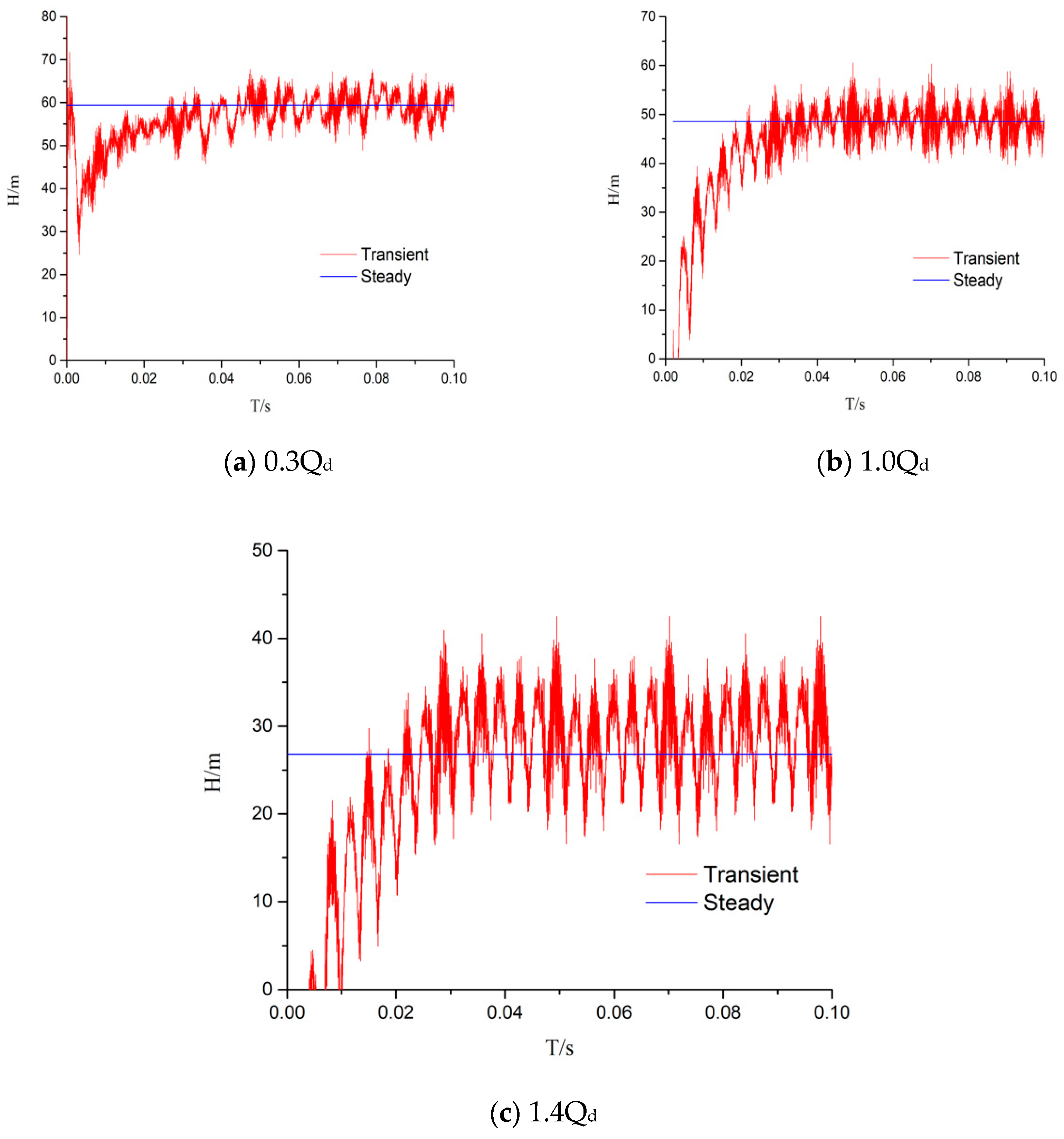
When the pump runs stably, the transient value of the head changes with time in a stable harmonic way, and the time-average value of the head is approximately equal to the steady state value. In one impeller rotation period, the number of head pulses corresponds to that of the impeller blades. The pulsation amplitude increases significantly with capacity.

(2)

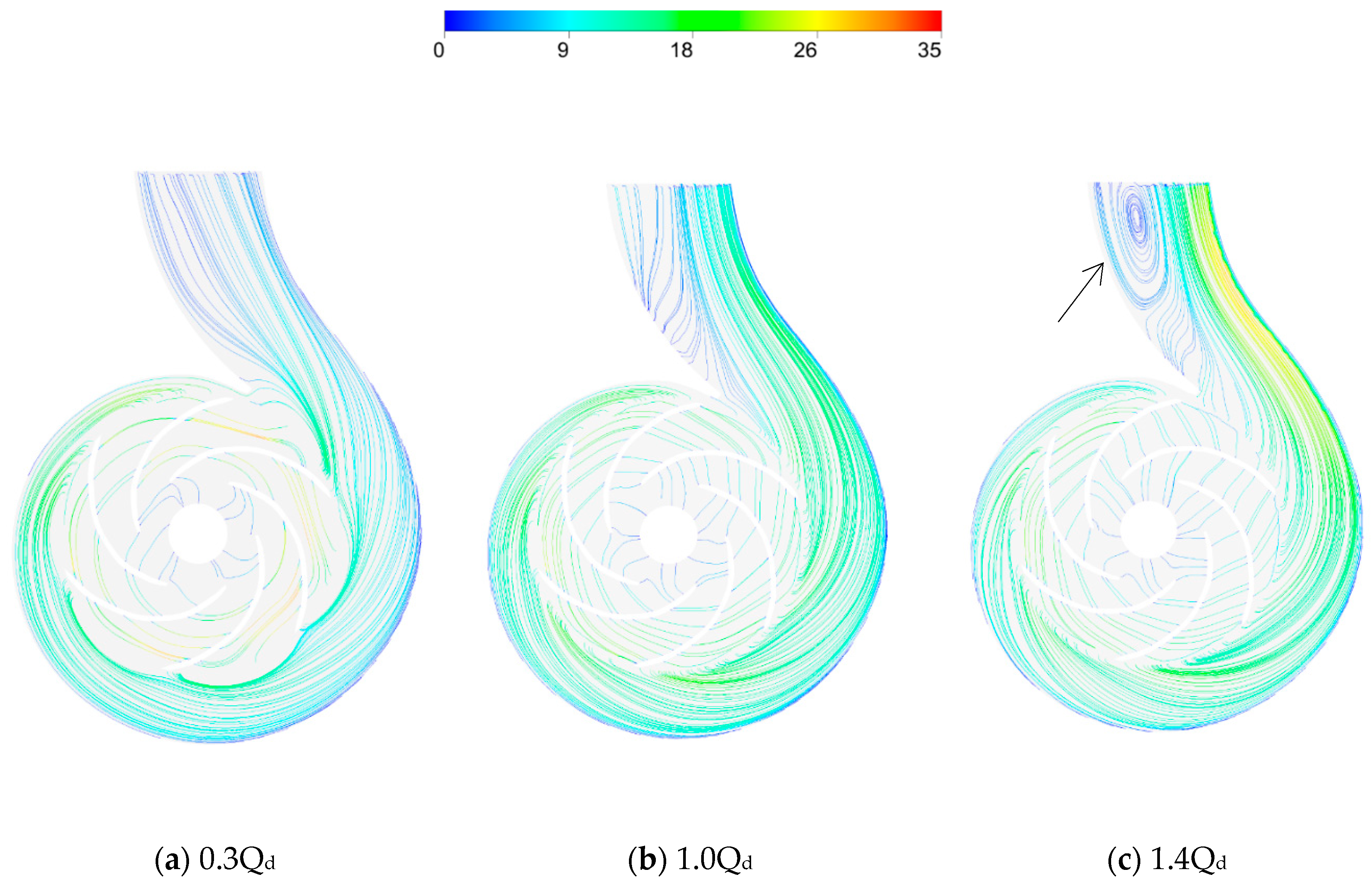
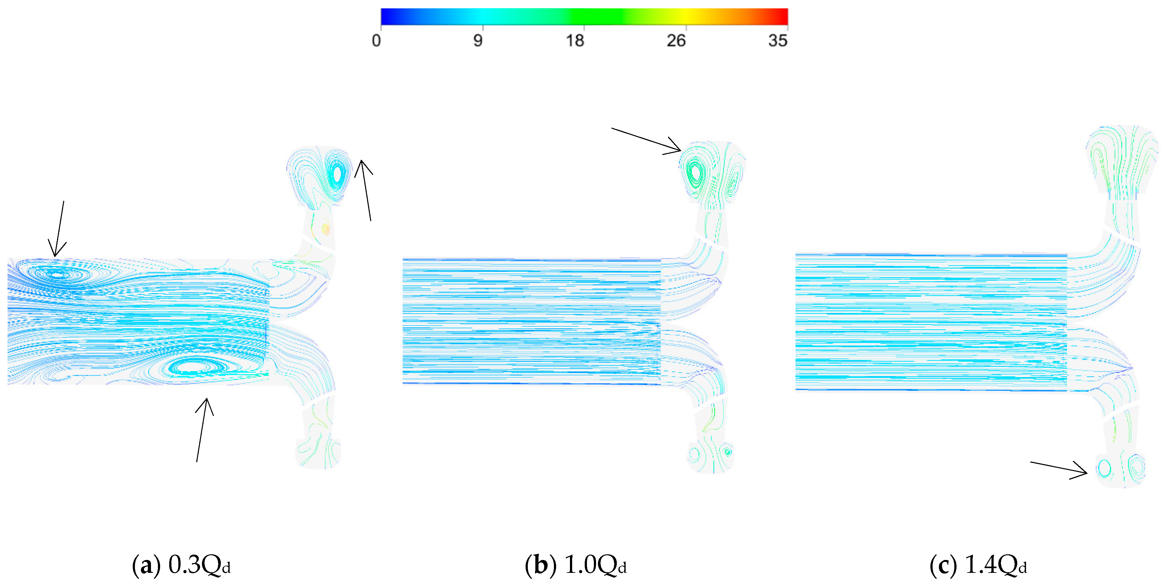
The flow simulation by OpenFOAM could well capture the vortexes in the pump. There are more vortexes under off-design conditions than those under design operating conditions. The flow velocity departing from the outlet of the impeller is more uniform under design operating conditions than those under off-design conditions. Diffusion loss and friction loss are the main hydraulic losses under lower and higher flow conditions, respectively.

(3)

The predicted results by OpenFOAM with the standard k-ε and the k-ω SST turbulence models agree well with the measured results of the pump characteristics in the current case.

(4)

The present study assumed that the inlet pressure was high enough to ensure no cavitation. In fact, cavitation always occurs and seriously affects pump performance. Thus, the effect of cavitation will be considered by OpenFOAM in further pump performance simulations.

References

1. Karassik, I.J.; Messina, J.P.; Cooper, P.; Heald, C.C. Pump Handbook; McGraw-Hill: New York, NY, USA, 2001; Volume 3. [Google Scholar]
2. Sakran, H.K. Numerical analysis of the effect of the numbers of blades on the centrifugal pump performance at constant parameters. Technology 2015, 6, 105–117. [Google Scholar]
3. Li, W.; Yang, C.; Yu, L.; Wang, G.; You, Y. Prediction on hydrodynamic performances of propeller by OpenFOAM. In Proceedings of the ASME 2009 28th International Conference on Ocean, Offshore and Arctic Engineering, Honolulu, HI, USA, 31 May–5 June 2009; pp. 633–638. [Google Scholar]
4. Petit, O.; Page, M.; Beaudoin, M.; Nilsson, H. The ERCOFTAC centrifugal pump OpenFOAM case-study. In Proceedings of the 3rd IAHR International Meeting of the Workgroup on Cavitation and Dynamic Problem in Hydraulic Machinery and Systems, Brno, Czech Republic, 14–16 October 2009. [Google Scholar]
5. Petit, O.; Nilsson, H. Numerical investigations of unsteady flow in a centrifugal pump with a vaned diffuser. Int. J. Rotating Mach. 2013, 2013. [Google Scholar] [CrossRef]
6. Nilsson, H. Evaluation of OpenFOAM for CFD of turbulent flow in water turbines. In Proceedings of the 23nd IAHR symposium on Hydraulic Machinery and Systems, Yokohama, Japan, 17–21 October 2006. [Google Scholar]
7. Xie, S. Studies of the ERCOFTAC Centrifugal Pump with OpenFOAM. Master’s Thesis, Chalmers University of Technology, Gothenburg, Sweden, 2010. [Google Scholar]
8. Zhang, H.; Zhang, L. Numerical simulation of cavitating turbulent flow in a high head Francis turbine at part load operation with OpenFOAM. Procedia Eng. 2012, 31, 156–165. [Google Scholar] [CrossRef]
9. Nuernberg, M.; Tao, L. Three dimensional tidal turbine array simulations using OpenFOAM with dynamic mesh. Ocean Eng. 2018, 147, 629–646. [Google Scholar] [CrossRef] [Green Version]
10. Liu, H.L.; Yun, R.E.N.; Kai, W.A.N.G.; Wu, D.H.; Ru, W.M.; Tan, M.G. Research of inner flow in a double blades pump based on OpenFOAM. J. Hydrodyn. Ser. B 2012, 24, 226–234. [Google Scholar] [CrossRef]
11. Nallasamy, M. Turbulence models and their applications to the prediction of internal flows: A review. Comput. Fluids 1987, 15, 151–194. [Google Scholar] [CrossRef]
12. Shojaeefard, M.H.; Tahani, M.; Ehghaghi, M.B.; Fallahian, M.A.; Beglari, M. Numerical study of the effects of some geometric characteristics of a centrifugal pump impeller that pumps a viscous fluid. Comput. Fluids 2012, 60, 61–70. [Google Scholar] [CrossRef]
13. Patankar, S.V.; Spalding, D.B. A calculation procedure for heat, mass and momentum transfer in three-dimensional parabolic flows. Int. J. Heat Mass Transf. 1972, 15, 1787–1806. [Google Scholar] [CrossRef]
14. Demirdzic, I.; Gosman, A.D.; Issa, R.I.; Peric, M. A calculation procedure for turbulent flow in complex geometries. Comput. Fluids 1987, 15, 251–273. [Google Scholar] [CrossRef]
15. Patankar, S. Numerical Heat Transfer and Fluid Flow; CRC Press: Boca Raton, FL, USA, 1980. [Google Scholar]
16. Luo, J.Y.; Gosman, A.D. Prediction of impeller-induced flow in mixing vessels using multiple frames of reference. Inst. Chem. Eng. Symp. Ser. 1994, 136, 549–556. [Google Scholar]
17. Farrell, P.E.; Maddison, J.R. Conservative interpolation between volume meshes by local Galerkin projection. Comput. Methods Appl. Mech. Eng. 2011, 200, 89–100. [Google Scholar] [CrossRef]
18. Versteeg, H.K.; Malalasekera, W. An Introduction to Computational Fluid Dynamics: The Finite Volume Method; Pearson Education: London, UK, 2007. [Google Scholar]
19. Jasak, H. Error Analysis and Estimation for the Finite Volume Method with Applications to Fluid Flows. Bachelor’s Thesis, Department of Mechanical Engineering Imperial College of Science, London, UK, 1996. [Google Scholar]
20. Auvinen, M.; Ala-Juusela, J.; Pedersen, N.; Siikonen, T. Time-accurate turbomachinery simulations with Open-Source® CFD: Flow analysis of a single-channel pump with OpenFOAM®. In Proceedings of the ECCOMAS CFD 2010, Lisbon, Portugal, 14–17 June 2010. [Google Scholar]
21. Arnone, A.; Pacciani, R. Rotor-stator interaction analysis using the Navier-Stokes equations and a multigrid method. J. Turbomach. 1996, 118, 679–689. [Google Scholar] [CrossRef]
22. Dawes, W.N. A simulation of the unsteady interaction of a centrifugal impeller with its vaned diffuser: Flow analysis. J. Turbomach. 1995, 117, 213–222. [Google Scholar] [CrossRef]
23. Huang, S.; Ruan, Z.; Liu, L. Performance predication of piping centrifugal pumps using computational fluid dynamics (CFD) technique. Chem. Eng. Mach. 2009, 2, 128–130. [Google Scholar]
24. Cheah, K.W.; Lee, T.S.; Winoto, S.H.; Zhao, Z.M. Numerical flow simulation in a centrifugal pump at design and off-design conditions. Int. J. Rotating Mach. 2007, 2007, 1–8. [Google Scholar] [CrossRef]
25. Limbach, P.; Kimoto, M.; Deimel, C.; Skoda, R. Numerical 3D simulation of the cavitating flow in a centrifugal pump with low specific speed and evaluation of the suction head. In Proceedings of the ASME Turbo Expo 2014: Turbine Technical Conference and Exposition, Dusseldorf, Germany, 16–20 June 2014. [Google Scholar]
26. Shim, H.S.; Kim, K.Y. Evaluation of Rotor-Stator interface models for the prediction of the hydraulic and suction performance of a centrifugal pump. J. Fluids Eng. 2019, 141, 111106. [Google Scholar] [CrossRef]
Figure 1. Geometry of type IS125-100.
Processes 07 00605 g001
Figure 2. Curves of grids independency.
Processes 07 00605 g002
Figure 3. Unstructured grids in the computational domain.
Processes 07 00605 g003
Figure 4. Velocity vectors in the pump (steady-state, OpenFOAM k-ε).
Processes 07 00605 g004
Figure 5. Distribution of streamlines in the pump on the xy plane (steady-state, OpenFOAM k-ε).
Processes 07 00605 g005
Figure 6. Distribution of streamlines in the pump on the zx plane (steady-state, OpenFOAM k-ε).
Processes 07 00605 g006
Figure 7. Static pressure distribution in the pump (steady-state, OpenFOAM k-ε).
Processes 07 00605 g007
Figure 8. Variation of calculated value H with time t (OpenFOAM k-ε).
Processes 07 00605 g008
Figure 9. Comparisons between predicted and tested performances.
Processes 07 00605 g009