Article

Temporal Feature Selection for Multi-Step Ahead Reheater Temperature Prediction

1
School of Comuputer Science and Engineering, Central South University, Changsha 410000, China
2
School of Mechanical Engineering and Automation, Zhejiang Sci-Tech. University, Hangzhou 310000, China
3
School of Automation, Central South University, Changsha 410000, China
*
Author to whom correspondence should be addressed.
Processes 2019, 7(7), 473; https://doi.org/10.3390/pr7070473
Submission received: 27 March 2019 / Revised: 5 June 2019 / Accepted: 5 June 2019 / Published: 22 July 2019

Abstract

:
Accurately predicting the reheater steam temperature over both short and medium time periods is crucial for the efficiency and safety of operations. With regard to the diverse temporal effects of influential factors, the accurate identification of delay orders allows effective temperature predictions for the reheater system. In this paper, a deep neural network (DNN) and a genetic algorithm (GA)-based optimal multi-step temporal feature selection model for reheater temperature is proposed. In the proposed model, DNN is used to establish a steam temperature predictor for future time steps, and GA is used to find the optimal delay orders, while fully considering the balance between modeling accuracy and computational complexity. The experimental results for two ultra-super-critical 1000 MW power plants show that the optimal delay orders calculated using this method achieve high forecasting accuracy and low computational overhead. Moreover, it is argued that the similarities of the two reheater experiments reflect the common physical properties of different reheaters, so the proposed algorithms could be generalized to guide temporal feature selection for other reheaters.

1. Introduction

Steam reheating plays an important role in power plants. It can increase thermal efficiency by 2% and it can also reduce steam humidity and improve the safety of the final stage’s blade [1,2]. However, due to the complexity of the many influential factors, it is difficult to maintain the reheat steam temperature within a certain range [3]. For instance, the reheater steam temperature of two ultra-super-critical 1000 MW units investigated in this paper may fluctuate between 565 °C and 610 °C, while the normal reheater outlet steam temperature is 603 °C with tolerable fluctuation within the range of 503 to 608 °C [4] (the specific threshold may vary with the type of reheater). A temperature that is too high will cause damage to the metal material, while a temperature that is too low will reduce the thermal cycle efficiency [5]. Therefore, finding features that affect the modeling target and analyzing the extent of these features are crucial for the system’s safety and efficiency.
A reheater system is a typical nonlinear hysteresis thermal system, which is highly coupled, complex, and impacted by many factors [6,7]. The selection of the most related features from a large variety of sensors is important for the realization of effective control [8]. Traditional feature selections are normally developed on the basis of mass balance, energy balance, and dynamic principles, which rely greatly on human expertise and normally require a long modeling time [9,10,11]. Recently, researchers have increasingly adopted the data-driven methodology that extracts features directly from huge amounts of accumulated process data [12,13,14]. Li et al. [15] analyzed operation parameters in power plants by correlation analysis to improve boiler efficiency. Wei et al. [16] used principle component analysis to transform higher-dimensional original data to lower-dimensional principle components, which were employed as the inputs to the N O x emission model to reduce memory storage requirements and computational costs for data analytics. Buczyński et al. [17] judged whether features could exert substantial effects on a CFD (phase fluidised bed)-based model using sensitivity analysis to predict the performance of a domestic central-heating boiler fired with solid fuels. Pisica et al. [18] chose mutual information to assess the relevance of feature subsets in order to determine the operating states of power systems. Wang et al. [19] utilized the outputs of an improved random forest algorithm as inputs of a back propagation neural network to weight the importance of features and to improve the prediction accuracy of N O x .
The above research works mainly focused on finding the most related features with respect to the modeling target, which only explores one dimension from all possible relationships. In practice, for the complex process, each feature may have a temporal effect on the modeling target [20]. For instance, some features might have a rapid impact on the target, while some other features might only display certain time-delay effects, i.e., effects after a certain period of time. In order to cover the temporal effects, multi-step features are often accumulated for data-driven modeling in the feature engineering process. Normally, the larger the delay order (number of steps selected) of a feature is, the more information it contains [21]. However, overly large delay orders of features may lead to overfitting, which may cause poor performance on unseen instances [22] and significantly increase memory storage and computational complexity for data analysis [23]. Therefore, it is necessary to find an optimal delay order set for each feature while maintaining a good balance between modeling accuracy and computational economy.
A few researchers have investigated the temporal feature selection problem. Lv et al. [21] used particle swarm optimization to determine delay orders and used a least square support vector machine (SVM) to predict the bed temperature of circulating fluidized bed boilers. However, this method suffered from computational complexity when modeling large-scale data sets. Shakil et al. [24] applied genetic algorithms to estimate the time delay of soft sensors for N O x and O 2 . Although these studies achieved good results on the delay order selection, their modeling targets were only for one particular future time instance, which has the potential not to include the features that impose too rapid or too slow impacts on the target. These approaches also provided little discussion on whether the generated delay order could be used to guide future modeling processes for similar equipment.
To address the optimal feature selection of delay orders for multi-step prediction, a method that combines a deep neural network (DNN) and a genetic algorithm (GA) is proposed. A prediction target with multiple future time steps is introduced to explore features that have rapid or slow effects. A DNN model is used to establish a steam temperature predictor [25] for the next 20 steps. A GA is proposed to find the optimal delay orders with the objective function of balancing modeling accuracy and computational complexity. The proposed method is tested in two 1000 MW coal-fired power plants, namely unit 3 and unit 4, which use more than two million records. The results of the two units display similar sets of delay orders for each feature, reflecting that the physical properties of reheater steam systems are similar to some extent.
The rest of this paper is organized as follows: Section 2 briefly describes the reheater system and proposes the problem statement. Section 3 establishes an objective function for model evaluation. The detailed introduction of the delay order selection mechanism is provided in Section 4. Section 5 presents experiments and discussions. Discussions and possible directions for future work are provided in the final section.

2. System Description and Problem Statement

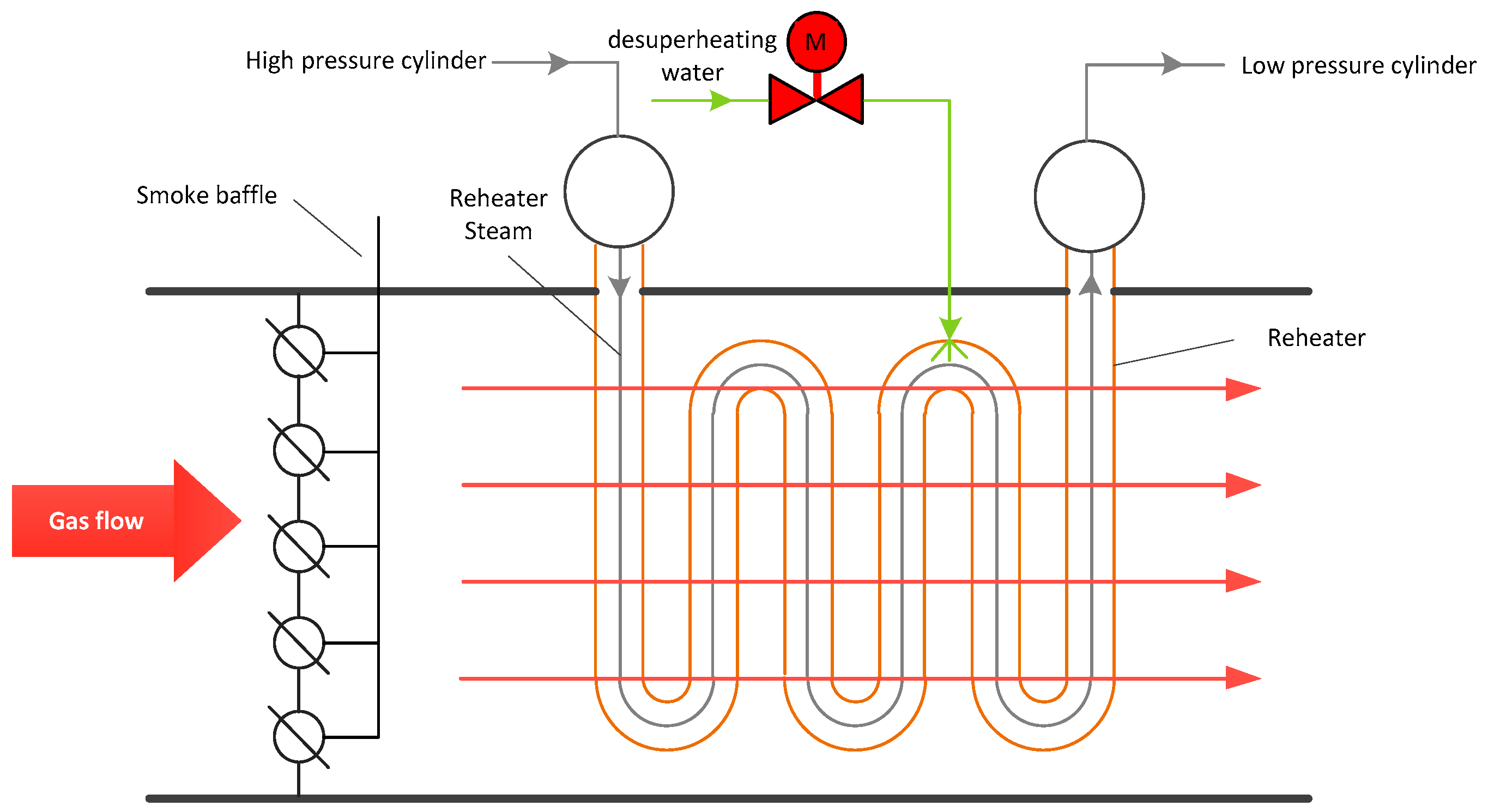
2.1. Description of Reheater System

A reheater is a set of tubes located in a boiler, the main purpose of which is to avoid excess moisture in steam at the end of expansion to protect the turbine. The exhaust steam from the high-pressure turbines passes through these heated tubes to collect more energy before driving the intermediate- and then low-pressure turbines. The conceptual structure of the reheater unit is shown in Figure 1.
After the high-pressured turbine, the exhaust pressure and temperature at the inlet of the reheater are about 35–37 kg/cm2 and 345–355 °C, respectively. A reheater is designed in the shape of a serpentine tube in order to increase the heated area. The hot smoke generated by the combustion of coal transfers heat to the reheater, meaning that the temperature of steam in the reheater rises. The steam temperature at the outlet of the reheater is kept around 603 °C. Reheater steam with high-temperature and high-pressure characteristics is collected into the high-temperature reheat steam container. A similar process is performed again in the low-pressure cylinder.
Table 1 denotes the influential features of our modeling target, which is the outlet steam temperature of the reheater. Many features affect the reheat steam temperature, such as the inlet steam temperature, inlet gas temperature, smoke baffle opening, etc. Also, these variables have different inertias toward the reheater outlet steam temperature. Therefore, these variables and their hysteresis times should be considered in the prediction model. Here, the previous values of the steam outlet temperature are also used in the modeling process and the multi-step steam temperatures are used as the outputs of the model. In order to simplify our discussion, the major factors are referred to by the notations shown in Table 1.

2.2. Problem Statement

One of the major control concerns of a reheater is the stability of steam o . In respect to the reheater, some features are reheater-uncontrollable, e.g., smoke temperature and pressure. These features might influence the reheater wall temperature and then change the outlet steam temperature. Steam o has the characteristics of being non-linear and having a large inertia. Due to the change in operation conditions, it may deviate from the expected range. The normal operation changes the smoke flow toward the reheater by adjusting the smoke baffle opening degree. This operation exhibits a long delay before it imposes impacts on temperature. Another method is to spray the desuperheated water to the reheater steam. This method promptly lowers steam temperature, but also reduces the boiler’s efficiency. Considering the economic benefits, the first method is always used. The second method is employed only in an emergency, such as when the steam temperature is too high or the working condition is changing.
Similar to the control variables mentioned above, other features also have impacts characterized by different inertias toward the steam temperature. One major concern is the complexity of accurately determining the impact inertia of different features, which highly depends on the physical nature laws of the reheater as well as the operational conditions of the reheater, e.g., combustion stability. One natural choice is to use long delay orders to compose the model inputs. However, the indiscriminate delay order settings make the feature dimension very high and introduce considerable overheads for both storage and computation. Thus, it is important to select the most cost-effective delay order for features while keeping the system model accurate enough.

3. Objective Function for Model Evaluation

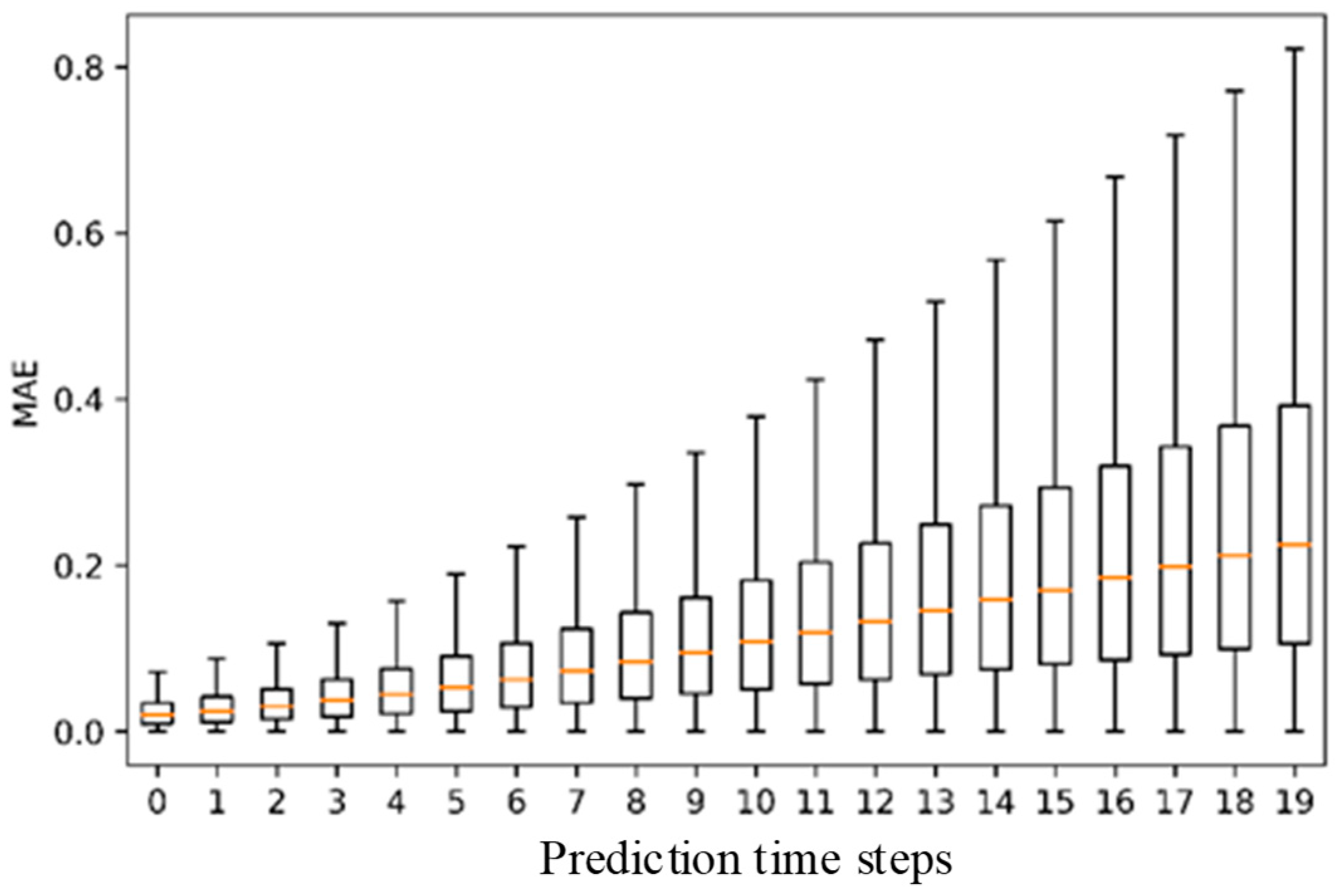
3.1. Multi-Step Prediction

In order to predict the temperature trend of steam o , the nonlinear autoregressive exogenous model is presented. Differing from other approaches, the proposed model predicts values not for any given time, but for a set of future moments.
Since the reheater system displays different hysteresis characteristics toward different features, modeling the steam o with both short and long hysteresis parameters is important. A multi-step steam o prediction model, which generates a serial of predictions for the next n + 1 time steps, is given in Equation (1).
[ y ^ ( t ) y ^ ( t + 1 ) ... y ^ ( t + n ) ] = f ( x 1 ( t 1 ) , , x 1 ( t τ 1 ) , , x k ( t 1 ) , , x k ( t τ k ) , y ( t 1 ) , , y ( t τ y ) ) ,
where t is the current time, t + n is the n-th future moment, x k is the k-th independent variable, y is a dependent variable, τ k represents the time delay order corresponding to x k , and τ y is the time delay order of dependent variable y.

3.2. Optimization Function

The prediction target increases the forecast performance for the next n + 1 time steps by selecting the most appropriate delay order. However, the total number of delay orders is proportional to the computational complexity and opposite to the model accuracy. Thus, the optimization goal defined is to strike a balance between the computational complexity and modeling accuracy. Accordingly, the objective function is used to minimize the total number of delay orders to minimize the computational complexity. Furthermore, the total number of delay orders is kept as high as possible but within a certain range in order to keep the prediction error low enough. Let ε be the maximum acceptable prediction error for the modeling target; thus, another optimization goal is transferred as one constraint, i.e., the prediction error is smaller than or equivalent to ε. Thus, a constrained optimization problem is formulated as Equation (2).
min J = τ y + k = 1 K τ k s . t . e = 1 m ( n + 1 ) | | Y ^ Y | | 1 e ε e l + 1 e l ,   l = 1 , 2 , , L 0 τ y τ k C
where K is the total delay orders of inputs, m is the total of test data, n is the n-th future moment, τ k is the delay order of x k , and τ y is the delay order of the dependent variable. J is the total of delay orders. e is the error in total m samples and n + 1 prediction numbers in the form of mean absolute error (MAE). e l   is the error generated by the l-th iteration. C is the max delay order. ɛ is the upper limit of MAE. Y ^ is the prediction value vector and Y ^ = [ y ^ ( t ) ,   y ^ ( t + 1 ) , , y ^ ( t + n ) ] T , Y is the actual value vector, and Y = [ y ( t ) ,   y ( t + 1 ) , , y ( t + n ) ] T ; Y ^ and Y have m samples.

4. Delay Order Selection

In order to accurately select the temporal features, two parts—i.e., the DNN-based prediction model and the GA-based optimal feature selection algorithm—are designed. First of all, the GA generates the individuals of different delay order combinations, which are used as the inputs to the DNN. Then, the DNN outputs the multi-step predictions, which are evaluated by the test sets. The evaluated values are employed as fitness values, which are used in the GA.

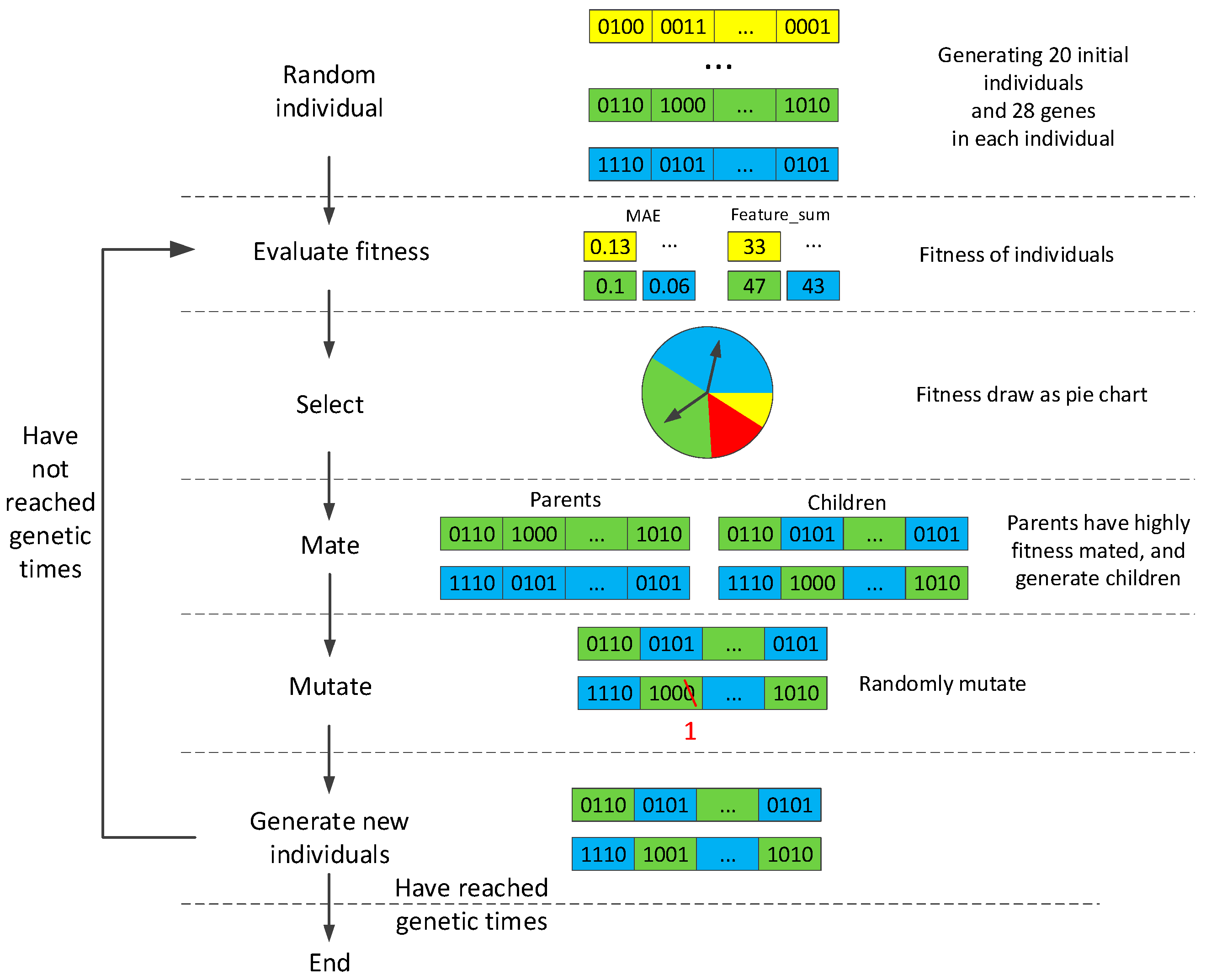
4.1. Delay Order Optimization

Delay order optimization is performed by the GA algorithm. The schema of GA is shown in Figure 2. The algorithm starts from an initial population with 20 individuals and each individual has 28 genes. These randomly generated genes are divided into seven sections. Each section represents an input parameter and has 4 binary numbers which can delay the order range from 0 to 15. Then, the individuals are evaluated by the fitness function, which returns two fitness values (MAE and the total of orders). The different fitness values are assigned different fitness scores. The smaller the MAE value, the higher the fitness scores. In a case in which the MAE values are very close (the difference is below a certain threshold), the smaller the total number of delay orders, the higher the fitness scores. The fitness score determines the probability of being selected as a parent. The probability of being selected is according to the roulette wheel selection, shown in Equation (3).
p i = f i j = 1 N f j ,
where N is the number of individuals in the population, f i is the fitness of individual i in the population, and p i is the probability of individual i being selected in the population.
Once the parents are selected, they have a certain probability ( p c ) of being mated randomly and generating new individuals. If the parents are not mated, they become new individuals in the new population. Then, the new population has a certain probability ( p m ) of deciding whether the individual is mutated. Mutating changes (0 changes to 1, or 1 to 0) randomly. The new individuals are evaluated, selected, mated, and mutated until the number of cycles is reached. At the end of the cycle, the GA obtains the best individuals [26,27].

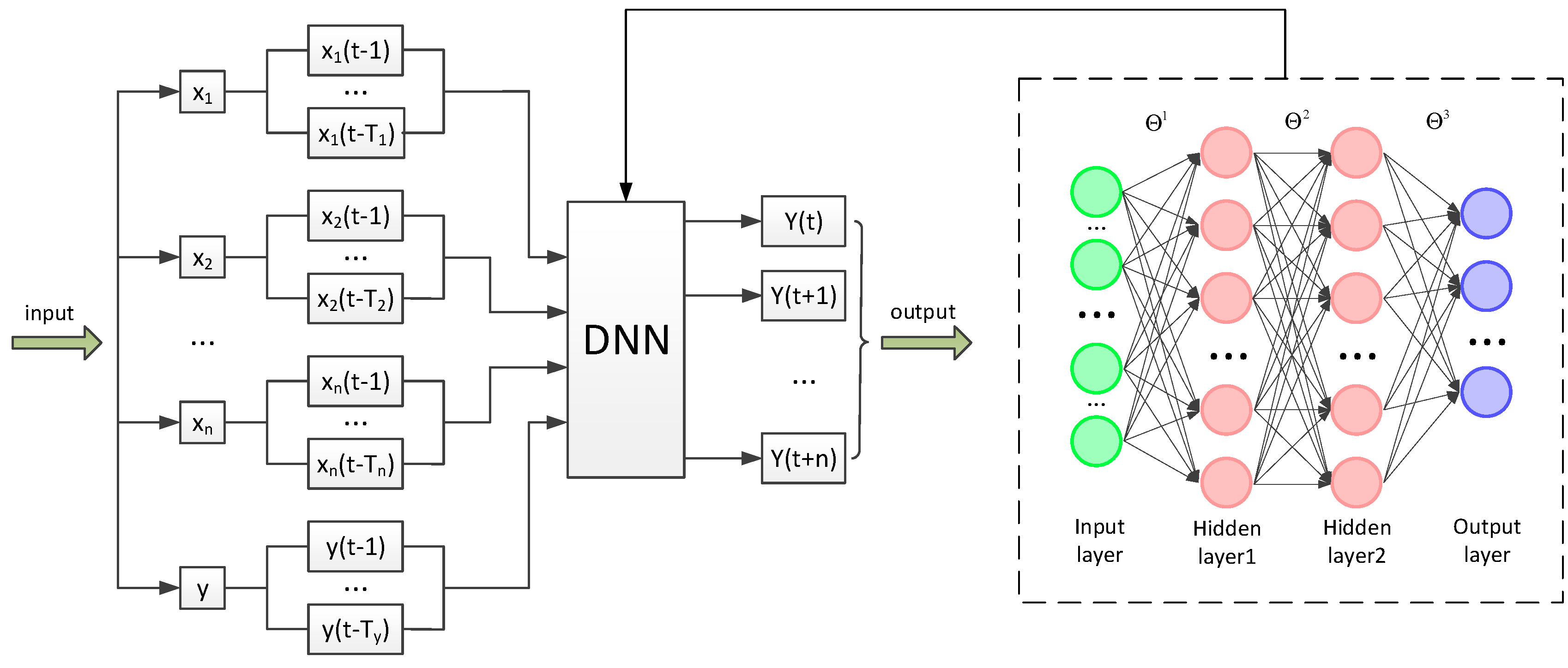
4.2. Prediction Model

DNN is used to fit the correlation between the future steam o and the historical reheater inlet variables with the accumulated data sets. Figure 3 is the structure of the steam o trend prediction model. Let m = τ 1 + τ 2 + + τ k be the total of input dimensions to DNN. The outputs of DNN are n + 1 values of steam o . DNN has one input layer, two hidden layers, one output layer, and a large number of neurons. The hypothesis function is shown in Equation (4).
h ( X ) = g ( Θ 3 g ( Θ 2 g ( Θ 1 X ) ) ) ,
where X is a vector with m dimensions and Θ 1 ,   Θ 2 , and Θ 3 are the weight matrixes between four layers, respectively. g() is the activation function.
The cost function of DNN is shown in Equation (5).
J ( θ ) = 1 2 m n i = 1 m j = 1 n [ h ( X j i ) Y j i ] 2 + λ L 2 ,
where m is the total number of samples, n is the total number of output variables, l k is the number of neurons in the k-th layer, and h ( X j i ) is the prediction value in the i-th sample and the j-th predict value. Y j i is the prediction value in the i-th sample and the j-th actual value, λ is the regularization parameter, and L2 is the regularization term to limit over-fitting. The goal of the DNN is to minimize Equation (5) with the given sets of features and training samples.

5. Experiments and Discussion

The data for modeling are collected every 3 s from unit 3 and unit 4 by the distributed control system (DCS). Unit 3 and unit 4 are two ultra-super-critical 1000 MW power plants with the same structure. In our experiment, in total, 7,084,800 records are used for evaluation, in which unit 3 and unit 4, respectively, have 3,542,400 records from 1 May 2016 to 31 August 2016.

5.1. Data Preprocessing

In the data preprocessing process, two steps are taken: Outlier removal and standardization.
Outlier removal: The outliers that violate the physical or technical limitations might affect the model’s performance and should be removed before modeling. (1) The points out of the normal range of physical or technical are replaced with the average of adjacent points. For instance, for a certain period, the temperature of steam o should be around 600 °C; thus, the points below 594 °C that violate the steady change characteristics of temperature should be replaced. (2) The errors of D water control time should be modified. Under normal circumstances, the D water control time (more than 0) takes a few minutes. For instance, if the collected data shows that the control time lasts for several hours, the abnormal control time will be modified to a maximum of 3 min.
Standardization: The different features might have different range of values. If these variables are used directly, the feature data with small values may be ignored, while the ones with large dimensions will be selected. Therefore, the Z-score standardization technique [28] is used to scale the data to the ones with a mean value of 0 and a standard deviation of 1, which will speed up the iteration rate of the optimization and convergence.

5.2. Experiment Settings

The parameters of DNN and GA are shown in Table 2. The DNN is a 2-hidden-layer neural network, and the learning rate is set to 0.001. MAE, which is the average absolute differences between predictions and actual observations, is used to evaluate the modeling error. Tanh is chosen as the activation function since it achieves the smallest average MAE compared to other activation functions (e.g., identity, logistic, relu) for the chosen data set.
The 4-month data for unit 3 and unit 4 are divided into 20 different sets. Each set consists of training data from 7 days (about 201,600 records) and test data from 1 day (about 28,800 records).

5.3. Results and Discussion

This proposed method is evaluated from three different perspectives: Firstly, a one-round simulation is performed with a set of data to demonstrate its capability for finding the optimal delay order for different features; secondly, the experiment is implemented on unit 3 and unit 4 at different times to demonstrate the adaptability of the presented method; finally, the delay order identified with data from the unit 3 is directly used in the modeling process for unit 4 to check its capability for generalization.
(1)
Results of the one-round simulation
As for getting the preliminary delay order in unit 3, the data from ~23 July 2016–30 July 2016 is selected as the experiment data. The changes of MAE and the total number of selected orders during the iteration process are shown in Figure 4a. The accuracy level of MAE is set as 0.001. In the early iterations, MAE begins to decrease while the total delay order increases. Then, until MAE stabilizes at 0.13—i.e., the lower limit of MAE—the total delay order decreases. In the later iterations, these criteria remain constant, which indicates that the algorithm is converged. Figure 4b shows each feature’s delay order. It can be seen that some features have a larger delay order, e.g., smoke p , which indicates large hysteresis, while in contrast, the order of D water shows timely but transient impacts.
In Figure 5, the forecasting errors in one-minute periods with 20 points in 30 July 2016 are plotted in a box plot which displays the distribution of five different metrics, i.e., minimum, first quartile, median, third quartile, and maximum. Figure 5 shows that MAE increases with the increase in the predicting time step. This is normal, as timely response factors, such as steam p , smoke t , and baffle o , cannot be captured by predictor. However, the median MAE in one minute is less than 0.3 °C, and the average is near 0.1 °C. According to Figure 4b, the maximum delay order of the reheater steam temperature steam o is 13. This means that the historical data of steam o have major impacts on the accuracy of the model. It also shows that, in the current system, steam o is not well controlled, as it should kept steady around 600 °C.
(2)
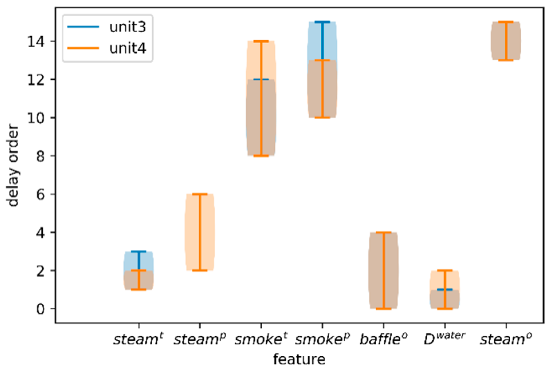
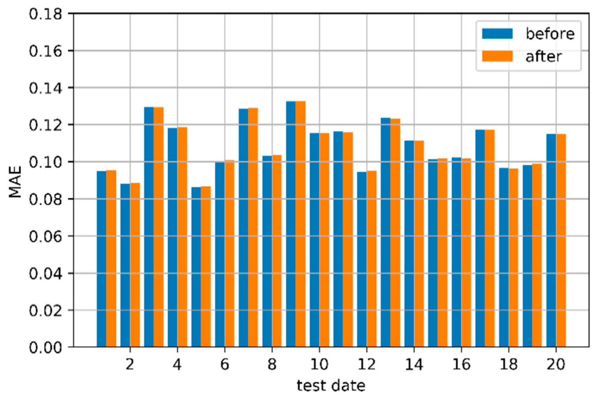
Comparisons of unit 3 and unit 4 from different perspectives
The feature selection method is tested for both unit 3 and unit 4 based on the operational data from 1 May 2016 to 31 August 2016. Since the records from some days contain too many abnormal data, the data from those days are not used for the model training. As shown in Table 3, the data periods are closed from the intra-comparisons within unit 3 or unit 4 or the inter-comparison between those two units.
Table 3 shows that the general range of the seven studied features has the corresponding length of delay orders with respect to their inertia toward steam o . For all 20 tests, there is no significant deviation regarding MAE. This means that the designed DNN with the selected features as the inputs achieves good convergence. It also shows that the delay orders of smoke t and smoke p are larger than those of steam t and steam p , as the smoke has indirect impacts toward the steam o . Thus, their delay orders are much larger than those of the feature of the inlet steam. D water has a very small delay order due to the fast temporal response toward steam o . For certain periods, the delay orders of D water are zero, e.g., in tests 9, 10, 16, and 18. The zero value is due to the lack of training data for D water . In those periods, the action of spraying de-superheated water is seldom performed. This is due to the insufficient training samples. At these stages, the numbers of sprays are, respectively, 31, 22, 26, and 18, while other tests have about 60 actions, owing to the comparable steam o which is more stable. A similar phenomenon can also be observed for the optimal delay order for   baffle o . These results show the importance of the data coverage for the accuracy of feature selection.
(3)
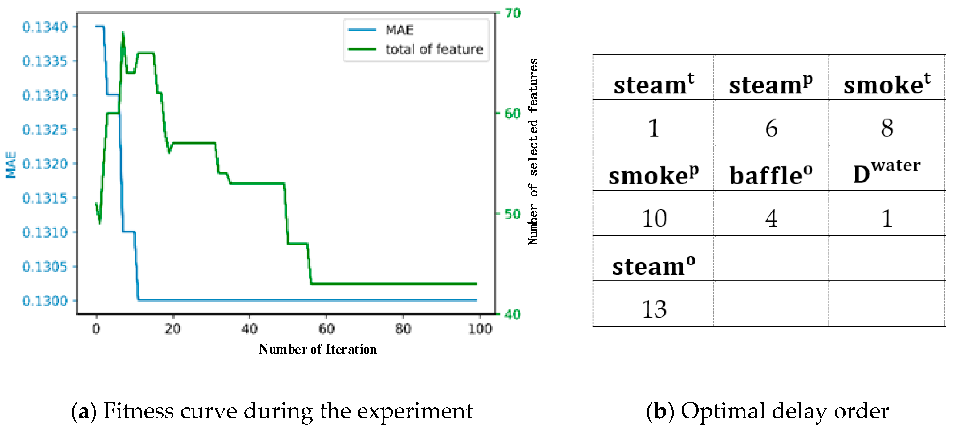
Determination of delay order
For the purpose of controlling steam o changes within the ideal range, properly finding a delay order is crucial to accurately describing the hysteresis of features for a prediction model. The variations of delay orders for each feature are shown in Figure 6; the shadow ranges from the maximum to minimum delay order. There is a large overlap between two units, which indicates the existence of common delay orders. The medians of overlap (2, 6, 10, 10, 2, 1, and 14) represent the general level of intervals and may serve as the references for delay orders regarding the steam o system of ultra-super-critical 1000 MW power plants.
The features with delay orders of 2, 6, 10, 10, 2, 1, and 14 generated from the data from unit 3 are used as selected features for the reheater steam temperature prediction. We also adopt the same methods to find the optimal feature distributed for the unit 4. Then, those results are compared with the dataset of test 1 to test 20, which are from unit 4. The orange bars indicate the MAE with the identified delay order. The directly calculated optimal solution is shown by the blue bars. Figure 7 shows the comparisons, which obviously indicate that the MAEs of two cases are approximately equal. The maximum error is only 0.9% (on the 16th day), which means that it is almost the same as the results from the optimal solutions. This shows that the selected delay orders (2, 6, 10, 10, 2, 1, and 14) have good generalization capability, and can, it is argued, represent the physical characteristics of two reheaters.

6. Conclusions

For many industrial processes, it is important to find the best feature delay orders as well as features that are most correlated with the prediction targets. In this paper, a delay order identification method based on GA and DNN is proposed. This method adopts the GA to generate candidate feature sets which try to find minimal numbers of features while keeping the MAE of the prediction model low enough. The DNN model is used for modeling processes that generate the multi-step predictions typically demanded in many industrial processes. This method is evaluated with experiments from different perspectives; data from two similar units are used to check whether the found time delays indeed demonstrate the physical characteristics of the underlying systems. The experimental results indicate that two units have similar delay orders and the delay order can be directly used for modeling similar devices with little loss of accuracy.
Of course, many interesting issues still need to be investigated. For instance, our solution limits the temporal feature selection. It is important for the delay order selection method to support both spatial and temporal feature selection. We are investigating the use of an attention mechanism to find the optimal solution for both dimensions. In addition, the GA demands considerable resources and computational costs. We are working to design more computationally efficient methods, e.g., filter-based feature selection for industrial feature processing.

Author Contributions

N.G. proposed the main idea of the method; J.L. and Z.Q. implemented the model and validated the field test. W.G. provided the funding.

Funding

This work is funded by the Nature Science Foundation of China 61403429, 61621062 and 61772473.

Acknowledgments

This work is funded by the Nature Science Foundation of China 61403429, 61621062 and 61772473.

Conflicts of Interest

The authors declare no conflict of interest.

References

  1. Zhang, L. Principle of Boiler; China Machine Press: Beijing, China, 2011. [Google Scholar]
  2. Ge, Z.; Zhang, F.; Sun, S.; He, J.; Du, X. Energy Analysis of Cascade Heating with High Back-Pressure Large-Scale Steam Turbine. Energies 2018, 11, 119. [Google Scholar] [CrossRef]
  3. Lee, K.Y.; Ma, L.; Boo, C.J.; Jung, W.H.; Kim, S.H. Intelligent modified predictive optimal control of reheater steam temperature in a large-scale boiler unit. In Proceedings of the 2009 IEEE Power & Energy Society General Meeting, Calgary, AB, Canada, 26–30 July 2009. [Google Scholar]
  4. Fan, Q.G. Principle of Boiler; China Electric Power Press: Beijing, China, 2014. [Google Scholar]
  5. Khartchenko, N.V.; Kharchenko, V.M. Advanced Energy Systems; CRC Press: Cleveland, OH, USA, 2013. [Google Scholar]
  6. Hogg, B.W.; El-Rabaie, N.M. Multivariable generalized predictive control of a boiler system. IEEE Trans. Energy Convers. 1991, 6, 82–288. [Google Scholar] [CrossRef]
  7. Liu, X.J.; Kong, X.B.; Hou, G.L.; Wang, J.H. Modeling of a 1000 MW power plant ultra super-critical boiler system using fuzzy-neural network methods. Energy Convers. Manag. 2013, 65, 518–527. [Google Scholar] [CrossRef]
  8. Suryanarayana, G.; Lago, J.; Geysen, D.; Aleksiejuk, P.; Johansson, C. Thermal load forecasting in district heating networks using deep learning and advanced feature selection methods. Energy 2018, 157, 141–149. [Google Scholar] [CrossRef]
  9. Staehelin, C.; Schultze, M.; Kondorosi, É.; Mellor, R.B.; Boiler, T.; Kondorosi, A. Structural modifications in Rhizobium meliloti Nod factors influence their stability against hydrolysis by root chitinases. Plant J. 1994, 5, 319–330. [Google Scholar] [CrossRef]
  10. Gnanapragasam, N.V.; Reddy, B.V. Numerical modeling of bed-to-wall heat transfer in a circulating fluidized bed combustor based on cluster energy balance. Int. J. Heat Mass Transf. 2008, 51, 5260–5268. [Google Scholar] [CrossRef]
  11. Black, S.; Szuhánszki, J.; Pranzitelli, A.; Ma, L.; Stanger, P.J.; Ingham, D.B.; Pourkashanian, M. Effects of firing coal and biomass under oxy-fuel conditions in a power plant boiler using CFD modelling. Fuel 2013, 113, 780–786. [Google Scholar] [CrossRef]
  12. Guyon, I.; Elisseeff, A. An introduction to variable and feature selection. J. Mach. Learn. Res. 2003, 3, 1157–1182. [Google Scholar]
  13. Saeys, Y.; Inza, I.; Larrañaga, P. A review of feature selection techniques in bioinformatics. Bioinformatics 2007, 23, 2507–2517. [Google Scholar] [CrossRef] [Green Version]
  14. Chandrashekar, G.; Sahin, F. A survey on feature selection methods. Comput. Electr. Eng. 2014, 40, 16–28. [Google Scholar] [CrossRef]
  15. Li, J.Q.; Gu, J.J.; Niu, C.L. The Operation Optimization based on Correlation Analysis of Operation Parameters in Power Plant. In Proceedings of the 2008 International Symposium on Computational Intelligence and Design, Wuhan, China, 17–18 October 2008. [Google Scholar]
  16. Wei, Z.; Li, X.; Xu, L.; Cheng, Y. Comparative study of computational intelligence approaches for NOx reduction of coal-fired boiler. Energy 2013, 55, 683–692. [Google Scholar] [CrossRef]
  17. Buczyński, R.; Weber, R.; Szlęk, A. Innovative design solutions for small-scale domestic boilers: Combustion improvements using a CFD-based mathematical model. J. Energy Inst. 2015, 88, 53–63. [Google Scholar] [CrossRef]
  18. Pisica, I.; Taylor, G.; Lipan, L. Feature selection filter for classification of power system operating states. Comput. Math. Appl. 2013, 66, 1795–1807. [Google Scholar] [CrossRef]
  19. Wang, F.; Ma, S.; Wang, H.; Li, Y.; Qin, Z.; Zhang, J. A hybrid model integrating improved flower pollination algorithm-based feature selection and improved random forest for NOX emission estimation of coal-fired power plants. Measurement 2018, 125, 303–312. [Google Scholar] [CrossRef]
  20. Sun, L.; Li, D.; Lee, K.Y. Enhanced decentralized PI control for fluidized bed combustor via advanced disturbance observer. Control Eng. Pract. 2015, 42, 128–139. [Google Scholar] [CrossRef]
  21. Lv, Y.; Hong, F.; Yang, T.; Fang, F.; Liu, J. A dynamic model for the bed temperature prediction of circulating fluidized bed boilers based on least squares support vector machine with real operational data. Energy 2017, 124 (Suppl. C), 284–294. [Google Scholar] [CrossRef]
  22. Galicia, H.J.; He, Q.P.; Wang, J. A reduced order soft sensor approach and its application to a continuous digester. J. Process Control 2011, 21, 489–500. [Google Scholar] [CrossRef]
  23. Souza, F.; Santos, P.; Araújo, R. Variable and delay selection using neural networks and mutual information for data-driven soft sensors. In Proceedings of the 2010 IEEE 15th Conference on Emerging Technologies & Factory Automation (ETFA 2010), Bilbao, Spain, 13–16 September 2010. [Google Scholar]
  24. Shakil, M.; Elshafei, M.; Habib, M.A.; Maleki, F.A. Soft sensor for NOx and O2 using dynamic neural networks. Comput. Electr. Eng. 2009, 35, 578–586. [Google Scholar] [CrossRef]
  25. Xia, C.; Wang, J.; McMenemy, K. Short, medium and long term load forecasting model and virtual load forecaster based on radial basis function neural networks. Int. J. Electr. Power Energy Syst. 2010, 32, 743–750. [Google Scholar] [CrossRef] [Green Version]
  26. Gosselin, L.; Tye-Gingras, M.; Mathieu-Potvin, F. Review of utilization of genetic algorithms in heat transfer problems. Int. J. Heat Mass Transf. 2009, 52, 2169–2188. [Google Scholar] [CrossRef]
  27. Woodward, R.I.; Kelleher, E.J.R. Towards ‘smart lasers’: Self-optimisation of an ultrafast pulse source using a genetic algorithm. Sci. Rep. 2016, 6, 37616. [Google Scholar] [CrossRef] [PubMed]
  28. Kreszig, E. Advanced Engineering Mathematics, 4th ed.; Wiley: Weinheim, Germany, 1979; p. 880. [Google Scholar]
Figure 1. Reheater structure.
Processes 07 00473 g001
Figure 2. The schematic schema of the genetic algorithm (GA)-based optimized feature selection algorithm. MAE(mean absolute error).
Processes 07 00473 g002
Figure 3. Multi-step prediction model for steam o . DNN—deep neural network.
Processes 07 00473 g003
Figure 4. Results for the one-round simulation for unit 3 (~23 July 2016–30 July 2016).
Processes 07 00473 g004
Figure 5. The box error curve.
Processes 07 00473 g005
Figure 6. Delay order distribution of the seven features.
Processes 07 00473 g006
Figure 7. Comparisons between optimal and proposed methods. Blue bars are the MAE of the optimal solution and the orange bars indicate the MAE of the proposed method.
Processes 07 00473 g007
Table 1. Influential parameters for the temperature of the outlet steam.
FeatureUnitInertiaNot.
Inlet steam temperature°Csmall Steam t
Inlet steam pressureMpasmall Steam p
Inlet smoke temperature°Clarge S moke t
Inlet smoke pressureKpasmall Smoke p
Smoke baffle opening%small Baffle o
Desuperheated water flowt/hlarge D water
Reheater steam temperature°C- Steam o
Table 2. The parameters of DNN and GA.
Neutral NetworkValueGAValue
Number of hidden layers2Number of initial individuals20
Number of first/second layer neurons42/23Mate rate0.5
Number of outputs20Mutate rate0.2
Activation functiontanhNumber of genes0–15
SolversgdIterations100
Learning_rate0.001 Ε 0.14
Λ0.0001--
Table 3. Results for both unit 3 and 4 (value before “/” is for unit 3 and after is for unit 4). MAE—Mean absolute error.
TestSample Date S t e a m t S t e a m p S m o k e t S m o k e p B a f f l e o D w a t e r S t e a m o MAE
1/118 May–15 May/1 May–8 May1/16/69/810/104/41/115/130.095/0.116
2/1216 May–23 May/17 May–24 May1/26/29/810/114/01/115/150.088/0.094
3/1320 May–27 May/24 May–31 May1/16/68/810/104/41/113/130.129/0.123
4/149 June–16 June/5 June –12 June3/16/612/810/130/41/113/130.118/0.111
5/1517 June–24 June/8 June–15 June1/16/49/1413/104/41/115/150.086/0.101
6/161 July–8 July/16 June–23 June3/16/69/815/104/01/015/130.100/0.101
7/1722 July–29 July/17 July–24 July1/16/212/1110/100/01/213/150.128/0.117
8/186 August–13 August/24 July–31 July1/16/29/1210/134/01/015/130.103/0.095
9/1910 August–17 August/5 August –12 August1/26/68/1013/104/20/113/150.132/0.115
10/2013 August–20 August/17 August–24 August1/26/68/910/104/20/115/140.115/0.115

