Article

Novel Parallel Heterogeneous Meta-Heuristic and Its Communication Strategies for the Prediction of Wind Power

1
College of Computer Science and Engineering, Shandong University of Science and Technology, Qingdao 266590, China
2
School of Software, Nanyang Institute of Technology, Nanyang 473004, China
*
Author to whom correspondence should be addressed.
Processes 2019, 7(11), 845; https://doi.org/10.3390/pr7110845
Submission received: 17 October 2019 / Revised: 7 November 2019 / Accepted: 7 November 2019 / Published: 11 November 2019
(This article belongs to the Special Issue Optimization Algorithms Applied to Sustainable Production Processes)

Abstract

:
Wind and other renewable energy protects the ecological environment and improves economic efficiency. However, it is difficult to accurately predict wind power because of the randomness and volatility of wind. This paper proposes a new parallel heterogeneous model to predict the wind power. Parallel meta-heuristic saves computation time and improves solution quality. Four communication strategies, which include ranking, combination, dynamic change and hybrid, are introduced to balance exploration and exploitation. The dynamic change strategy is to dynamically increase or decrease the members of subgroup to keep the diversity of the population. The benchmark functions show that the algorithms have excellent performance in exploration and exploitation. In the end, they are applied to successfully realize the prediction for wind power by training the parameters of the neural network.

1. Introduction

The world is facing the problem of resource shortages, and the utilization of renewable energy has become a hot research issue. Wind is a renewable clean energy with good economic condition and is rapidly developing. However, the large-scale application of wind power is limited due to volatility, intermittence and uncertainty. Therefore, the accurate prediction of wind power is considerable for the combination of power systems, optimizing energy market and reducing the cost of power reserve. Over the past decades, many models have been proposed to predict the wind power, which mainly include physical, statistical and intellectual learning methods [1,2,3,4,5,6].
The physical method is to establish the numerical weather prediction (NWP) model in the wind field and achieves the prediction by the parameters of wind turbines. The statistical method predicts wind power through constructing related mathematical functions. The methods of traditional statistics include time series models, regression analysis and so on, and they have complicated and poor prediction. In recent years, neural network (NN) has become popular because it can deal with the non-linear ability of data, and many models based on NN have been proposed to predict wind power. Since the speed and accuracy of NN are greatly affected by the related parameters, meta-heuristics are introduced to optimize the parameters of NN and implement the prediction [7].
Meta-heuristics are increasingly used to deal with optimization problems in engineering, production, and manufacturing. Their main purposes are to randomly search a large solution space and find the optimal solution or approximate one. Genetic algorithm (GA) simulates the natural evolutionary processes to search for the optimal solution [8,9,10,11,12]. Particle swarm optimization (PSO) derives from complex adaptive system (CAS) and finds the optimum by simulating the foraging behavior of birds [13,14,15,16,17,18,19,20]. Differential evolution (DE) is a random search algorithm based on group differences [21,22,23,24,25,26], and guides the finding direction through mutual cooperation and competition among individuals within the group. Grey wolf optimizer (GWO) is an algorithm which mimics the wolf pack hierarchy and hunting behavior [27,28,29,30,31]. QUasi-Affine TRansformation Evolutionary (QUATRE) is a new proposed optimization algorithm based on quasi-affine transformation and group coordination [32,33,34,35].
However, meta-heuristics generally have the problems of slow convergence and poor solution quality, and many researchers have taken many useful attempts in parallelization [36,37,38,39]. Schutte et al. [40] proposes the coarse-grained parallelization of PSO to solve the problems of large-scale data, low cost and multiple local optimal solutions. Penas et al. [26] improves the abilities of global search and local search through asynchronous parallel and cooperative island-model to achieve an appropriate balance. Pan et al. [41] adopts a parallel and compact method based on bat algorithm (BA) to increase the diversity of solution in searching space and achieves the sharing of computation. Alba et al. [42] summarizes the development and application scenarios of parallel meta-heuristic algorithms in recent years, as well as it introduces the future development trend and possible research routes.
The main contributions of this paper are summarized as follows:
  • It first proposes parallel heterogeneous model based on PSO and GWO.
  • It introduces four new communication strategies to improve the abilities of exploration and exploitation.
  • It dynamically changes the members of subgroup from the diversity of the population.
The rest of the paper is organized as follows. Section 2 describes the algorithms of PSO and GWO, and population-based parallelization. Section 3 introduces a new parallel heterogeneous model and four communication strategies. Section 4 testifies their performance by 28 benchmark functions. Section 5 realizes the prediction for wind power by the algorithms and neural network. Section 6 concludes the works of this paper and gives some advice regarding further work.

2. Preliminaries

Meta-heuristic algorithm is a combination of stochastic and local search. It gives a feasible solution to the problem under acceptable computational time and space, and the solution is not be predicted in advance. Meta-heuristics are divided into trajectory-based algorithm and population-based algorithm [43]. In this section, we firstly introduce the population-based algorithms, PSO and GWO. Secondly, we briefly describe the communication models and strategies for parallel.

2.1. Particle Swarm Optimization

PSO simulates a flock of birds through mass-less particles. Each particle has only two properties of speed and position, where speed is the direction of movement and position denotes the motion of particle. Each particle separately searches for the optimal solution in the space and takes the best individual extreme ever found as the current global optimal solution of the whole particles. They adjust their speeds and positions according to the extreme and the global optimal solution [13]. PSO has the characteristics of simplicity and fewer parameters. It has been widely used in functional optimization, training neural network, fuzzy system controlling and other applications.
PSO randomly initializes a group of particles and then iteratively finds the optimal solution. In each iteration, the particles update their speeds and positions with the following equations.
V i j ( t + 1 ) = w V i j ( t ) + c 1 r 1 ( p b e s t i j X i j ) + c 2 r 2 ( g b e s t j X i j )
X i j ( t + 1 ) = X i j ( t ) + V i j ( t + 1 )
where i j represents the j t h dimension of the i t h particle. t is the current iteration. r 1 and r 2 are two random numbers between [0, 1]. X denotes the position. V is the speed. p b e s t represents the extreme of an individual. g b e s t is the global optimal solution. c 1 and c 2 are coefficient. w is called the inertia factor, which is calculated as follows:
w = ( w m a x w m i n ) ( M A X _ I T i t ) / M A X _ I T + w m i n
where w m a x and w m i n respectively represent the maximum and minimum values of w. M A X _ I T is the maximum number of iteration. i t is the current number of iteration. Figure 1 shows the complete flow chart of PSO.

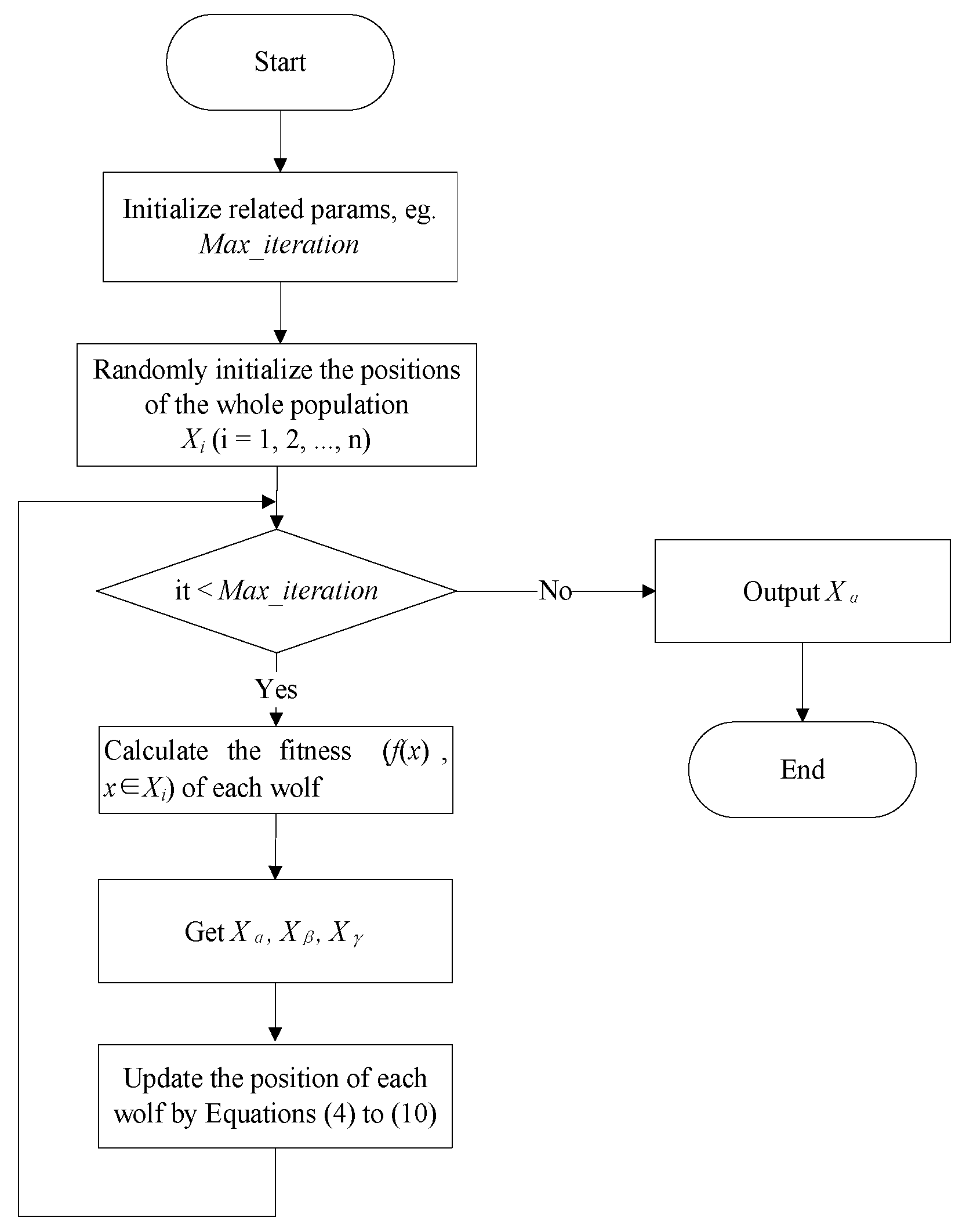
2.2. Grey Wolf Optimizer

The grey wolf pack has a very strict social hierarchy similar to the pyramid. GWO mimics the behaviors of grey wolf, such as social hierarchy, searching and hunting prey [27]. GWO refers to the first three optimal solutions respectively named alpha ( α ), beta ( β ) and delta ( δ ). The remaining candidates are collectively referred to as omega ( ω ) wolves, and the omegas update their places by the positions of the three optimal solutions. GWO has the characteristics of strong convergence, few parameters and easy realization. A wolf first computes its distance from α , β and δ by Equations (4)–(9), then its position is updated through Equation (10). Figure 2 shows the complete flow chart of GWO.
D α = | 2 r 2 · X α X i |
D β = | 2 r 2 · X β X i |
D δ = | 2 r 2 · X δ X i |
X 1 = X α ( 2 a · r 1 a ) · D α
X 2 = X β ( 2 a · r 1 a ) · D β
X 3 = X δ ( 2 a · r 1 a ) · D δ
X i ( t + 1 ) = X 1 + X 2 + X 3 3
where X α , X β and X δ respectively represent the positions of α , β and δ . D α , D β and D δ are the distances between α , β , δ and i. With the iteration process, a decreases linearly from 2 to 0. r 1 and r 2 are two random numbers between [0, 1].

2.3. Population-Based Parallelization

Parallel algorithms are generally superior to their corresponding non-parallel in efficiency, scalability, or solution quality. Most of them are homogeneous, so their parallelization is to implement multiple serial versions of them at the same time. Parallel algorithms not only effectively reduce the computational cost, but also further improve the solution quality. Because meta-heuristics often fall into local optimum, parallel algorithms could search for solution in more space. Therefore, they are increasingly used to solve complex global optimization problems.

2.3.1. Communication Models

Population parallelization is an important strategy, and the population is divided into several independent subgroups. Lalwani et al. [44] proposes four communication models based on [45].
  • Star model
One subgroup acts as the master node, while the others as slave nodes accept the control of it. Instead of directly communicating among the subgroups, the global information is exchanged through the master node, as shown in Figure 3a.
  • Migration model
Each subgroup communicates with only two ones around it to form a ring structure. Therefore, the optimal information is passed throughout the whole subgroups, as shown in Figure 3b.
  • Diffusion model
Each subgroup communicates with the others, and the global information is transmitted by broadcasting, as shown in Figure 3c.
  • Hybrid model
It is a hybrid model of migration and diffusion. Each subgroup communicates with only four subgroups around it, as shown in Figure 3d.

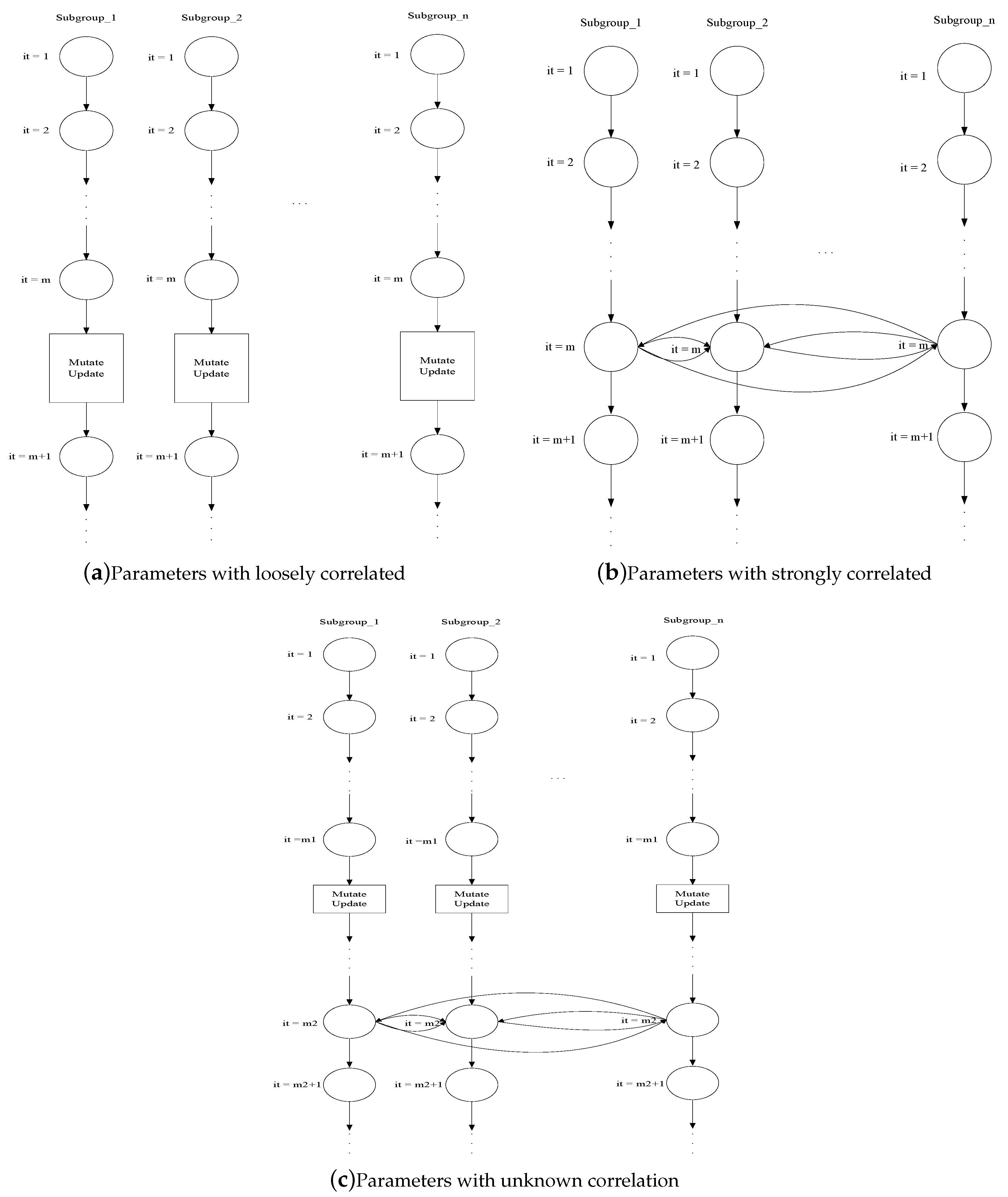
2.3.2. Communication Strategies

Chang et al. [16] proposes three communication strategies to improve the solution quality by the correlations of subgroups.
  • Parameters with loosely correlated
If the subgroups are not closely related or independent, they develop independently; but after m iterations, the worst t of each subgroup are eliminated, as shown in Figure 4a.
  • Parameters with strongly correlated
If the subgroups are strongly related, they communicate after m iterations, and the worst t of each subgroup are replaced by the best t of the others, as shown in Figure 4b.
  • Parameters with unknown correlation (Hybrid)
If we do not know the correlations between the subgroups, we take a hybrid strategy based on the two strategies, as shown in Figure 4c.

3. Novel Parallel Heterogeneous Algorithm

Meta-heuristic algorithm tends to fall into the trap of premature convergence, because it is possible that the fitness of an individual greatly exceeds the average of the population, which makes the individual be rapidly replicated and propagated in the population. It leads to a decline in the diversity of the population and a loss the evolutionary capacity. In parallel algorithms, if a subgroup falls into the premature trap and it does not affect the ability of others to find the optimal solution, it is a useful way. In the next section, we propose a novel parallel heterogeneous algorithm and four new communication strategies to improve the solution quality.

3.1. The Model of Parallel Heterogeneous Algorithm

In the traditional population-based parallelization, each subgroup adopts the same meta-heuristic in the parallel algorithm. Although it avoids the premature trap, it has common defects owing to the subgroups using the same algorithm. For example, it is not high of the search accuracy of PSO; GWO has slow convergence in the late and it is lack of the necessary information exchange between the pack.
The subgroups adopt different algorithms in parallel heterogeneous proposed by this paper. So if the parallel algorithm adopts the migration model, its corresponding model is shown in Figure 5. Subgroup 1 adopts meta-heuristic 1 and subgroup 2 uses meta-heuristic 2, and so on.
In the parallel heterogeneous model, subgroups use different algorithms. Although they do not avoid the inherent defects of the algorithms, they overcome the defects through parallelization, and they even be greatly improved by proper communication strategies. Parallel heterogeneous model takes advantage of the characteristics of different algorithms and balances their defects. It solves a variety of problems and searches for the optimal solution in the space by various methods, but it is difficult to coordinate the subgroups because of different algorithms with diverse parameters and models. In the following section, it describes how to achieve information exchange between subgroups.

3.2. New Communication Strategies

Even if some of the subgroups stagnate in local optimum, a parallel algorithm also has a chance to acquire the global optimum. This is because information exchange can change the distribution of subgroups. So a good communication strategy undertakes the algorithm converge quickly and avoids falling into local optimum.

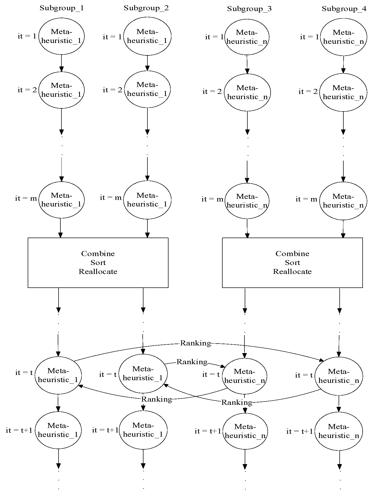
3.2.1. Communication Strategy with Ranking

The worst individuals are replaced by the best ones of other subgroups. This greatly advances the fitness of a subgroup. The subgroup is strongly influenced by its neighbors, that is, it is improved by more experienced neighbors, but it is also degenerated by inexperienced neighbors. After the replacement is complete, it ranks its neighbors. The ranking equation is described as follows.
r a n k i n g = 1 i f   ( f ¯ > f ¯ ) 0 i f   ( f ¯ = f ¯ ) 1 i f   ( f ¯ < f ¯ )
where f ¯ is the average fitness of the subgroup; f ¯ is the new average value of the subgroup.
After m iterations, the worst individuals of each subgroup are eliminated and its neighbors receive the ranking. Then they judge whether to mutate or not by the ranking, as shown in Figure 6. The strategy estimates the subgroups and accelerates the evolution of the ones with poor convergence.

3.2.2. Communication Strategy with Combination

In the strategy, subgroups communicate with others according to the similarities and differences of the meta-heuristics. Subgroups which use the same algorithm have the same parameters and models, so their solutions are comparable. They are merged, sorted and then allocated to each subgroup in turn. After communication, the solutions of subgroups become random, and there are not large differences between each subgroup. The strategy widely finds the optimal solution in the search space and avoids falling into local optimum, as shown in Figure 7.
By reallocating members, the strategy makes the subgroups jump out of local trap, and they explore in more space, so that the convergences of them remain roughly the same. The pseudo code of combination is described in Algorithm 1.
Algorithm 1 Combination
 //ngroups.number is the number of subgroups
for g = 1 : ngroups.number do
  //ngroups.algorithms is the number of meta-heuristics
  for j = 1 : ngroups.algorithms do
   if j == groups(g).algorithm then
    //ngroups.size is the number of subgroup
    for l = 1 : ngroups.size do
     temp(j,t(j)) = groups(g).pop(l);
     t(j) = t(j) + 1;
    end for
   end if
  end for
end for
for j = 1 : ngroups.algorithms do
  i = 1;
  temp(j) = SortPopulationByFitness(temp(j));
  for g = 1 : ngroups.number do
   if j == groups(g).algorithm && it(j) then
    groups(g).pop(p(g)) = temp(j,i);
    i = i + 1;
    p(g) = p(g) + 1;
   end if
  end for
end for

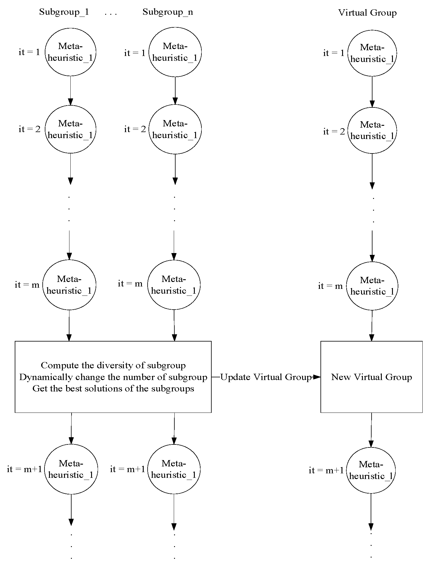
3.2.3. Communication Strategy with Dynamic Change

Individuals are affected by the best fitness of individual in the population, which causes the individuals to move and quickly converge at an optimum in the search space. Through adding perturbations, increasing search space and maintaining the population diversity, the population is prevented from falling into local optimum. The diversity of population is expressed by the distribution of fitness values in the population.
S = 1 n i = 1 n ( f i f ¯ ) 2
where n is number of the population; f i is the fitness of the i t h individual; and f ¯ is the average of the population.
With the evolution of the algorithm, if it decreases in the diversity of the population, it is necessary to add dynamically individuals to the population; if the diversity increases, it is reduced by appropriately decreasing individuals. Increasing members avoids falling into local optimum through searching in wide space; while decreasing members speeds up the convergence. However, this will reduce the convergence rate of the population, so a virtual population is set up, which is composed of the optimal solutions of the subgroups. They do not guide the search direction of the subgroups, but they search in the known potential optimal space. The members of the virtual population are updated once every m iterations. Its pseudo code is described in Algorithm 2.
The communication strategy effectively maintains the diversity of the population and finds a better balance between exploration and exploitation, as shown in the Figure 8.
Algorithm 2 Dynamic Change
 Sort A //A is the best solutions of the subgroups
 Sort B // B is the virtual group
for i = 1 : length(A), j = 1 : length(B) do
  if f(A(i)) < B(j) then
   B(j) = A(i);
   ++i;
  else
   ++j;
  end if
end for

3.2.4. Hybrid Communication Strategy

The hybrid strategy adopts a combination for the subgroups with the same algorithms, and uses ranking for the subgroups having different algorithms, so it has the advantages of two strategies. It keeps the diversity differences of the subgroups, and provides the coordination of all ones. It promotes them with poor search abilities, so that the population searches quickly in the space and avoids falling into local optimum. Suppose there are four subgroups, subgroups 1 and 2 adopt meta-heuristic 1, subgroups 3 and 4 adopt meta-heuristic n. After m iterations, the population executes communication strategy with ranking. After t iterations, the population implements communication strategy with combination, as shown in the Figure 9.

4. Experimental Results and Analysis

In this section, we use 28 benchmark functions to test the effectiveness of the proposed parallel heterogeneous model and communication strategies. The functions, listed in Table 1, Table 2, Table 3 and Table 4, have the classifications of unimodal, multimodal, fixed-dimension and composite problems. S p a c e is the boundary of its search range; D i m represents the dimension of the function and f m i n indicates the optimum.

4.1. Parameters Configuration

For verifying the results, we compare them with PGWO, which is a parallelized GWO that the poorer agents in a subgroup are replaced by the best agents of its neighbor. The parallel heterogeneous model uses the algorithms of GWO and PSO. They run 30 times and 500 iterations on each benchmark function. Each subgroup has 30 individuals. They have 4 subgroups and replace the three worst individuals every four iterations. Subgroups 1 and 2 adopt GWO; subgroups 3 and 4 adopt PSO. Table 5 lists the parameters of PSO and other parameters. Where b e t a is a scaling factor; p c R is a mutant constant and g r o u p _ s i z e is the number of subgroup.
Table 6 shows the final solution of each function, and various statistical measures from average (AVG) and standard deviation (STD) show that the proposed algorithms outperform PGWO in the unimodal, multimodal and composite functions and they have the competitive ability. Figure 10, Figure 11, Figure 12 and Figure 13 demonstrate the solution qualities and speeds of the benchmark functions. The X-axis represents the iteration numbers and the Y-axis denotes the corresponding fitness.

4.2. Unimodal Functions

f 1 to f 6 are unimodal functions. They have no local solution, and there is only one global solution. So they are usually used to examine the convergence rates of algorithms. From Table 6 and Figure 10, the proposed algorithms perform better than PGWO except for f 6 . It shows that they utilize the advantages of different meta-heuristics. They not only converge quickly, but also quickly find the global optimum. PH-D does better in most functions, which means that the virtual population and the diversity quickly find the optimal solutions in the unimodal functions.

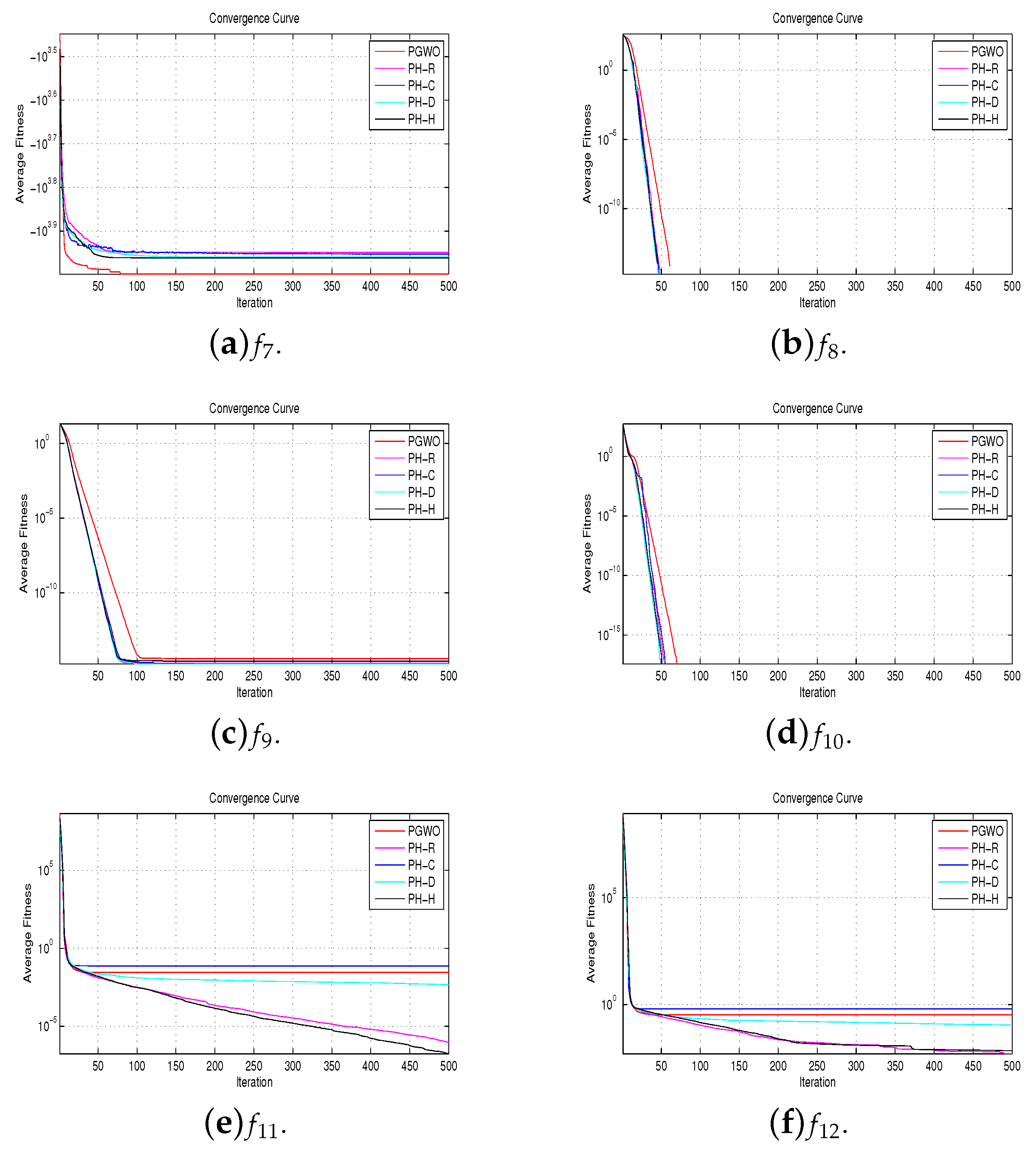
4.3. Multimodal Functions

f 7 to f 12 are multimodal functions. They have many local optimum and almost are most difficult to find the global optimal solution. From Table 6 and Figure 11, the algorithms perform well in the convergence rates except for f 7 . They have the abilities of escaping from local optimum and seeking out a near-global optimal solution. PH-C does better, which shows that maintaining population evolution is helpful in solving multi-dimensional problems.

4.4. Fixed-Dimension Multimodal Functions

f 13 to f 22 are fixed-dimension multimodal functions. They only have a few local minima, and the dimensions of the functions are small. From Table 6 and Figure 12, the algorithms have good performance; in particular, PH-C performs better in most functions. In the fixed-dimension multimodal functions, the convergence of the algorithm is guaranteed by keeping the diversity differences within the population and the limited differences among different populations.

4.5. Composite Multimodal Functions

f 23 to f 28 are composite multimodal functions. They have extremely complex structures with many randomly located global optimum and several randomly located deep local optimum. From Table 6 and Figure 13, they are not very good, but PGWO falls into local trap in f 26 and f 28 , while they do not. Due to the complex shape of the composition functions, it is difficult to get the accurate results from the functions. However, we conclude that PH-R and PH-H get relatively good results. In particular, in f 23 and f 27 they almost find the optimal solutions.
From the above discussion, the proposed algorithms prefer exploration at early stage and then gradually lessen their exploration rates to perform exploitation. In the later stage, they exploit the search space to find the optimal solution. Hence, it is adequate from the convergence curves that they improve the abilities of exploration and exploitation.

5. Application for Wind Power Forecasting

The prediction for wind power has important significance and practical values for the reasonable dispatch of wind power, reducing grid operation and maintenance costs, ensuring the reliability of power system and improving the economic and safety of wind turbine operation. In this section, we present the model for wind power prediction based on hybrid neural network and achieves the prediction.

5.1. The Model of Wind Power Forecasting Based on Hybrid Neural Network

Wind power brings great convenience to people because of its environmental protection, clean, renewable and other advantages. However, the shortcomings of wind power have an impact on the stability of the power system. Through the prediction for wind power, the power plan can be designedly arranged to avoid large fluctuations in the power grid.
Neural network (NN) is a hot research topic in the field of artificial intelligence. It has been successfully applied in many applications, such as engineering control, online learning and classification etc. [46]. NN has an input layer, one or more hidden layers and an output layer. It receives data from the input layer and outputs data through the output layer. Figure 14 shows the classical structure of the three layers network.
Where w and w are the weights of neural network.
The back propagation (BP) algorithm is usually to train the parameters of the network. It is a kind of supervised learning and requires labeled data. Its working principle is to adjust the parameters of the network by measuring variance and gradient descent. However, it has some inherent defects, such as easy falling into local minima, low precision, and learning speed. Meta-heuristics have been widely used in training NN because they can find global solution in the multi-dimensional search space. So we use the proposed methods to train the network and finish the prediction for wind power based on NWP. The model of the training parameters is shown in Figure 15.

5.2. Simulation Results

NWP data is acquired from Inner Mongolia wind farm every 10 min, and there is 600 to 1320 kw for the rated output power of wind turbine. Each set of data includes wind speed, wind direction sine, wind direction cosine, air pressure, temperature, humidity and density at different heights in multiple areas. Since there is a huge amount of data per day, adding too much data will reduce the generalization ability of the model. First, the incomplete data is removed, and then cluster analysis [47] is used to search for the samples that are the most similar to the predicted NWP data in the historical data. Figure 16 shows the chart of wind power forecasting system.

5.2.1. Data Preprocessing

We use the data 1 January 2015 to 31 August, where 210 days of data is randomly selected to train the model and then 30 days of data is used to predict. Because NN is sensitive to the data between [−1, 1]. At the input layer, the data is converted to the value of [−1, 1] by the following equation.
d = d ( d m a x + d m i n ) / 2 ( d m a x + d m i n ) / 2
where d is the current value; d is the converted result; d m a x and d m i n respectively represent the maximum and minimum values. The fitness is used to judge the performance of the NN. In this paper, we use the mean squared error to implement a better prediction.
f = 1 n ( i = 1 n ( y y ^ ) 2
where n is the number of prediction data; y indicates the actual result and y ^ presents its corresponding prediction. The range of f is limited to [0, 1].

5.2.2. The Evaluation Performance of Hybrid Model

The parameters of the algorithms are the same as Section 4.1. Their prediction accuracy is shown in the Table 7, where NN is the classical neural network.
Figure 17 and Figure 18 shows the prediction errors and results of the algorithms. From Table 7 and Figure 17 and Figure 18, it is high for the prediction accuracy of PH-R. The fluctuation trend of PH-R is closer to the real results, especially between the samples of 6th, 16th, 23rd and 29th. In general, when the actual wind power is low and the change is relatively stable, the prediction results are very close to the actual power; while the actual power drastically changes, they predict large deviations. Some optimization methods [48,49,50,51] may be adopted to further improve the efficiency of the proposed scheme in the future work.

6. Conclusions

Meta-heuristics use exploration and exploitation to find the optimal solution. The purpose of exploration is to locate promising areas within the search space and exploitation finds the optimal solution in the found promising areas. The key aspect of the algorithm is its ability to preserve the balance between exploration and exploitation during the optimization process. Because the parallel heterogeneous algorithm uses different meta-heuristics, it has certain advantages. Through using communication strategies, it improves the solution quality of the algorithm. We propose four strategies for keeping the population diversity and improving the convergence rate. It is very difficult to accurately predict wind power because of the influence of the natural environment. The algorithms train the neural network to implement the prediction. Simulation results show that they obtain a good result and reduce the error of prediction. There are many meta-heuristics, but in this paper we only use two algorithms. In the future, we can use more to get better performance in different fields and build more complex models to improve the accuracy of prediction.

Author Contributions

Conceptualization, P.H. and J.-S.P.; Sotftware, P.H.; Formal analysis, P.H. and S.-C.C.; Methodology, P.H., J.-S.P. and S.-C.C.; Writing—original draft, P.H.; Writing—review & editing, P.H., J.-S.P., S.-C.C.

Funding

This research received no external funding.

Conflicts of Interest

The authors declare no conflict of interest.

References

  1. Wang, S.; Zhang, N.; Wu, L.; Wang, Y. Wind speed forecasting based on the hybrid ensemble empirical mode decomposition and GA-BP neural network method. Renew. Energy 2016, 94, 629–636. [Google Scholar] [CrossRef]
  2. Zhou, W.; Lou, C.; Li, Z.; Lu, L.; Yang, H. Current status of research on optimum sizing of stand-alone hybrid solar–wind power generation systems. Appl. Energy 2010, 87, 380–389. [Google Scholar] [CrossRef]
  3. Bhaskar, K.; Singh, S. AWNN-assisted wind power forecasting using feed-forward neural network. IEEE Trans. Sustain. Energy 2012, 3, 306–315. [Google Scholar] [CrossRef]
  4. Liu, H.; Tian, H.Q.; Chen, C.; Li, Y.f. A hybrid statistical method to predict wind speed and wind power. Renew. Energy 2010, 35, 1857–1861. [Google Scholar] [CrossRef]
  5. Wang, J.; Zhou, Y. Multi-objective dynamic unit commitment optimization for energy-saving and emission reduction with wind power. In Proceedings of the 2015 5th International Conference on Electric Utility Deregulation and Restructuring and Power Technologies (DRPT), Changsha, China, 26–29 November 2015; pp. 2074–2078. [Google Scholar]
  6. Wang, C.N.; Le, T.M.; Nguyen, H.K.; Ngoc-Nguyen, H. Using the Optimization Algorithm to Evaluate the Energetic Industry: A Case Study in Thailand. Processes 2019, 7, 87. [Google Scholar] [CrossRef]
  7. Hu, P.; Pan, J.S.; Chu, S.C.; Chai, Q.W.; Liu, T.; Li, Z.C. New Hybrid Algorithms for Prediction of Daily Load of Power Network. Appl. Sci. 2019, 9, 4514. [Google Scholar] [CrossRef]
  8. Morris, G.M.; Goodsell, D.S.; Halliday, R.S.; Huey, R.; Hart, W.E.; Belew, R.K.; Olson, A.J. Automated docking using a Lamarckian genetic algorithm and an empirical binding free energy function. J. Comput. Chem. 1998, 19, 1639–1662. [Google Scholar] [CrossRef]
  9. Pan, J.; McInnes, F.; Jack, M. Application of parallel genetic algorithm and property of multiple global optima to VQ codevector index assignment for noisy channels. Electron. Lett. 1996, 32, 296–297. [Google Scholar] [CrossRef]
  10. Deb, K.; Pratap, A.; Agarwal, S.; Meyarivan, T. A fast and elitist multiobjective genetic algorithm: NSGA-II. IEEE Trans. Evol. Comput. 2002, 6, 182–197. [Google Scholar] [CrossRef]
  11. Shieh, C.S.; Huang, H.C.; Wang, F.H.; Pan, J.S. Genetic watermarking based on transform-domain techniques. Pattern Recognit. 2004, 37, 555–565. [Google Scholar] [CrossRef]
  12. Huang, H.C.; Pan, J.S.; Lu, Z.M.; Sun, S.H.; Hang, H.M. Vector quantization based on genetic simulated annealing. Signal Process. 2001, 81, 1513–1523. [Google Scholar] [CrossRef]
  13. Eberhart, R.; Kennedy, J. A new optimizer using particle swarm theory. In Proceedings of the Sixth International Symposium on Micro Machine and Human Science, Nagoya, Japan, 4–6 October 1995; pp. 39–43. [Google Scholar]
  14. Wang, H.; Sun, H.; Li, C.; Rahnamayan, S.; Pan, J.S. Diversity enhanced particle swarm optimization with neighborhood search. Inf. Sci. 2013, 223, 119–135. [Google Scholar] [CrossRef]
  15. Shi, Y.; Eberhart. Particle swarm optimization: Developments, applications and resources. In Proceedings of the 2001 Congress on Evolutionary Computation, Seoul, Korea, 27–30 May 2001; Volume 1, pp. 81–86. [Google Scholar]
  16. Chang, J.F.; Roddick, J.F.; Pan, J.S.; Chu, S. A parallel particle swarm optimization algorithm with communication strategies. J. Inf. Sci. Eng. 2005, 21, 809–818. [Google Scholar]
  17. Sun, C.L.; Zeng, J.C.; Pan, J.S. An improved vector particle swarm optimization for constrained optimization problems. Inf. Sci. 2011, 181, 1153–1163. [Google Scholar] [CrossRef]
  18. Wang, J.; Ju, C.; Ji, H.; Youn, G.; Kim, J.U. A Particle Swarm Optimization and Mutation Operator Based Node Deployment Strategy for WSNs; International Conference on Cloud Computing and Security; Springer: Boston, MA, USA, 2017; pp. 430–437. [Google Scholar]
  19. Liu, W.; Wang, J.; Chen, L.; Chen, B. Prediction of protein essentiality by the improved particle swarm optimization. Soft Comput. 2018, 22, 6657–6669. [Google Scholar] [CrossRef]
  20. Wang, J.; Ju, C.; Kim, H.j.; Sherratt, R.S.; Lee, S. A mobile assisted coverage hole patching scheme based on particle swarm optimization for WSNs. Clust. Comput. 2019, 22, 1787–1795. [Google Scholar] [CrossRef]
  21. Storn, R.; Price, K. Differential evolution—A simple and efficient heuristic for global optimization over continuous spaces. J. Glob. Optim. 1997, 11, 341–359. [Google Scholar] [CrossRef]
  22. Qin, A.K.; Huang, V.L.; Suganthan, P.N. Differential evolution algorithm with strategy adaptation for global numerical optimization. IEEE Trans. Evol. Comput. 2008, 13, 398–417. [Google Scholar] [CrossRef]
  23. Meng, Z.; Pan, J.S.; Kong, L. Parameters with adaptive learning mechanism (PALM) for the enhancement of differential evolution. Knowl.-Based Syst. 2018, 141, 92–112. [Google Scholar] [CrossRef]
  24. Meng, Z.; Pan, J.S.; Tseng, K.K. PaDE: An enhanced Differential Evolution algorithm with novel control parameter adaptation schemes for numerical optimization. Knowl.-Based Syst. 2019, 168, 80–99. [Google Scholar] [CrossRef]
  25. Das, S.; Suganthan, P.N. Differential evolution: A survey of the state-of-the-art. IEEE Trans. Evol. Comput. 2010, 15, 4–31. [Google Scholar] [CrossRef]
  26. Penas, D.R.; Banga, J.R.; González, P.; Doallo, R. Enhanced parallel differential evolution algorithm for problems in computational systems biology. Appl. Soft Comput. 2015, 33, 86–99. [Google Scholar] [CrossRef]
  27. Mirjalili, S.; Mirjalili, S.M.; Lewis, A. Grey wolf optimizer. Adv. Eng. Softw. 2014, 69, 46–61. [Google Scholar] [CrossRef]
  28. Mirjalili, S. How effective is the Grey Wolf optimizer in training multi-layer perceptrons. Appl. Intell. 2015, 43, 150–161. [Google Scholar] [CrossRef]
  29. Pan, J.S.; Dao, T.K.; Chu, S.C.; Nguyen, T.-T. A novel hybrid GWO-FPA algorithm for optimization applications. In Proceedings of the International Conference on Smart Vehicular Technology, Transportation, Communication and Applications, Kaohsiung, Taiwan, 6–8 November 2017; pp. 274–281. [Google Scholar]
  30. Song, X.; Tang, L.; Zhao, S.; Zhang, X.; Li, L.; Huang, J.; Cai, W. Grey Wolf Optimizer for parameter estimation in surface waves. Soil Dyn. Earthq. Eng. 2015, 75, 147–157. [Google Scholar] [CrossRef]
  31. El-Fergany, A.A.; Hasanien, H.M. Single and multi-objective optimal power flow using grey wolf optimizer and differential evolution algorithms. Electr. Power Components Syst. 2015, 43, 1548–1559. [Google Scholar] [CrossRef]
  32. Meng, Z.; Pan, J.S.; Xu, H. QUasi-Affine TRansformation Evolutionary (QUATRE) algorithm: A cooperative swarm based algorithm for global optimization. Knowl.-Based Syst. 2016, 109, 104–121. [Google Scholar] [CrossRef]
  33. Liu, N.; Pan, J.S.; Xue, J.Y. An Orthogonal QUasi-Affine TRansformation Evolution (O-QUATRE). In Proceedings of the 15th International Conference on IIH-MSP in Conjunction with the 12th International Conference on FITAT, Jilin, China, 18–20 July 2019; Volume 2, pp. 57–66. [Google Scholar]
  34. Pan, J.S.; Meng, Z.; Xu, H.; Li, X. QUasi-Affine TRansformation Evolution (QUATRE) algorithm: A new simple and accurate structure for global optimization. In Proceedings of the International Conference on Industrial, Engineering and Other Applications of Applied Intelligent Systems, Morioka, Japan, 2–4 August 2016; pp. 657–667. [Google Scholar]
  35. Meng, Z.; Pan, J.S. QUasi-Affine TRansformation Evolution with External ARchive (QUATRE-EAR): An enhanced structure for differential evolution. Knowl.-Based Syst. 2018, 155, 35–53. [Google Scholar] [CrossRef]
  36. Weber, M.; Neri, F.; Tirronen, V. Shuffle or update parallel differential evolution for large-scale optimization. Soft Comput. 2011, 15, 2089–2107. [Google Scholar] [CrossRef]
  37. Pooranian, Z.; Shojafar, M.; Abawajy, J.H.; Abraham, A. An efficient meta-heuristic algorithm for grid computing. J. Comb. Optim. 2015, 30, 413–434. [Google Scholar] [CrossRef]
  38. Yang, Z.; Li, K.; Niu, Q.; Xue, Y. A novel parallel-series hybrid meta-heuristic method for solving a hybrid unit commitment problem. Knowl.-Based Syst. 2017, 134, 13–30. [Google Scholar] [CrossRef]
  39. Mussi, L.; Daolio, F.; Cagnoni, S. Evaluation of parallel particle swarm optimization algorithms within the CUDA™ architecture. Inf. Sci. 2012, 181, 4642–4657. [Google Scholar] [CrossRef]
  40. Schutte, J.F.; Reinbolt, J.A.; Fregly, B.J.; Haftka, R.T.; George, A.D. Parallel global optimization with the particle swarm algorithm. Int. J. Numer. Methods Eng. 2004, 61, 2296–2315. [Google Scholar] [CrossRef] [PubMed] [Green Version]
  41. Pan, J.S.; Dao, T.K.; Nguyen, T.-T. A Novel Improved Bat Algorithm Based on Hybrid Parallel and Compact for Balancing an Energy Consumption Problem. Information 2019, 10, 194–215. [Google Scholar]
  42. Alba, E.; Luque, G.; Nesmachnow, S. Parallel metaheuristics: Recent advances and new trends. Int. Trans. Oper. Res. 2013, 20, 1–48. [Google Scholar] [CrossRef]
  43. Xue, X.; Chen, J. Optimizing ontology alignment through hybrid population-based incremental learning algorithm. Memetic Comput. 2019, 11, 209–217. [Google Scholar] [CrossRef]
  44. Lalwani, S.; Sharma, H.; Satapathy, S.C.; Deep, K.; Bansal, J.C. A Survey on Parallel Particle Swarm Optimization Algorithms. Arab. J. Sci. Eng. 2019, 44, 2899–2923. [Google Scholar] [CrossRef]
  45. Madhuri, D.K.; Deep, K. A state-of-the-art review of population-based parallel meta-heuristics. In Proceedings of the Nature & Biologically Inspired Computing, Coimbatore, India, 9–11 December 2009; pp. 9–11. [Google Scholar]
  46. Liao, D.Y.; Wang, C.N. Neural-network-based delivery time estimates for prioritized 300-mm automatic material handling operations. IEEE Trans. Semicond. Manuf. 2004, 17, 324–332. [Google Scholar] [CrossRef]
  47. Jeng-Shyang, P.; Lingping, K.; Tien-Wen, S.; Pei-Wei, T.; Waclav, S. α-fraction first strategy for hierarchical wireless sensor networks. J. Internet Technol. 2018, 19, 1717–1726. [Google Scholar]
  48. Nguyen, T.T.; Pan, J.S.; Dao, T.K. An Improved Flower Pollination Algorithm for Optimizing Layouts of Nodes in Wireless Sensor Network. IEEE Access 2019, 7, 75985–75998. [Google Scholar] [CrossRef]
  49. Pan, J.S.; Lee, C.Y.; Sghaier, A.; Zeghid, M.; Xie, J. Novel Systolization of Subquadratic Space Complexity Multipliers Based on Toeplitz Matrix-Vector Product Approach. IEEE Trans. Very Large Scale Integr. (VLSI) Syst. 2019. [Google Scholar] [CrossRef]
  50. Xue, X.; Chen, J.; Yao, X. Efficient User Involvement in Semiautomatic Ontology Matching. IEEE Trans. Emerg. Top. Comput. Intell. 2018. [Google Scholar] [CrossRef]
  51. Pan, J.S.; Kong, L.; Sung, T.W.; Tsai, P.W.; Snášel, V. A clustering scheme for wireless sensor networks based on genetic algorithm and dominating set. J. Internet Technol. 2018, 19, 1111–1118. [Google Scholar]
Figure 1. The complete flow chart of particle swarm optimization (PSO).
Processes 07 00845 g001
Figure 2. The complete flow chart of the grey wolf optimizer (GWO).
Processes 07 00845 g002
Figure 3. Communication models for population-based parallelization.
Processes 07 00845 g003
Figure 4. Communication strategies for population-based parallelization.
Processes 07 00845 g004
Figure 5. Parallel heterogeneous model.
Processes 07 00845 g005
Figure 6. Communication strategy with ranking.
Processes 07 00845 g006
Figure 7. Communication strategy with combination.
Processes 07 00845 g007
Figure 8. Communication strategy with dynamic change.
Processes 07 00845 g008
Figure 9. Hybrid communication strategy.
Processes 07 00845 g009
Figure 10. Convergence curves of unimodal benchmark functions.
Processes 07 00845 g010
Figure 11. Convergence curves of multimodal benchmark functions.
Processes 07 00845 g011
Figure 12. Convergence curves of fixed-dimension multimodal benchmark functions.
Processes 07 00845 g012
Figure 13. Convergence curves of composite benchmark functions.
Processes 07 00845 g013
Figure 14. The three-layer neural network structure.
Processes 07 00845 g014
Figure 15. The model of the training parameters.
Processes 07 00845 g015
Figure 16. Wind power forecasting system.
Processes 07 00845 g016
Figure 17. The prediction errors.
Processes 07 00845 g017
Figure 18. The prediction results.
Processes 07 00845 g018
Table 1. Unimodal benchmark functions.
FunctionSpaceDimfmin
( S p h e r e ) f 1 ( x ) = i = 1 n x i 2 [−100, 100]300
( S c h w e f e l s f u n c t i o n 2.21 ) f 2 ( x ) = i = 1 n | x i | + i = 1 n | x i | [−10, 10]300
( S c h w e f e l s p r o b l e m 1.2 ) f 3 ( x ) = i = 1 n ( j 1 i x j ) 2 [−100, 100]300
( S c h w e f e l s f u n c t i o n 2.22 ) f 4 ( x ) = m a x i { | x i | , 1 i n } [−100, 100]300
( S t e p ) f 5 ( x ) = i = 1 n ( [ x i + 0.5 ] ) 2 [−100, 100]300
( D e j o n g s n o i s y ) f 6 ( x ) = i = 1 n i x i 4 + r a n d o m [ 0 , 1 ) [−1.28, 1.28]300
Table 2. Multimodal benchmark functions.
FunctionSpaceDimfmin
( S c h w e f e l ) f 7 ( x ) = i = 1 n x i s i n ( | x i | ) [−500, 500]30−12,569
( R a s t r i n g i n ) f 8 ( x ) = i = 1 n [ x i 2 10 c o s ( 2 π x i ) + 10 ] [−5.12, 5.12]300
( A c k l e y ) f 9 ( x ) = 20 e x p ( 0.2 1 n i = 1 n x i 2 ) e x p ( 1 n i = 1 n c o s ( 2 π x i ) ) + 20 + e [−32, 32]300
( G r i e w a n k ) f 10 ( x ) = 1 4000 i = 1 n x i 2 i = 1 n c o s ( x i i ) + 1 [−600, 600]300
( G e n e r a l i z e d p e n a l i z e d 1 ) f 11 ( x ) = π n { 10 s i n ( π y 1 ) + i = 1 n 1 ( y i 1 ) 2 [ 1 + 10 s i n 2 ( π y i + 1 ) ] + ( y n 1 ) 2 } + i = 1 n u ( x i , 10 , 100 , 4 ) y i = 1 + x i + 1 4 u ( x i , a , k , m ) = k ( x i a ) m x i > a 0 a < x i < a k ( x i a ) m x i < a [−50, 50]300
( G e n e r a l i z e d p e n a l i z e d 2 ) f 12 ( x ) = 0.1 { s i n 2 ( 3 π x 1 ) + i = 1 n ( x i 1 ) 2 [ 1 + s i n 2 ( 3 π x i + 1 ) ] + ( x n 1 ) 2 [ 1 + s i n 2 ( 2 π x n ) ] } + i = 1 n u ( x i , 10 , 100 , 4 ) [−50, 50]300
Table 3. Fixed-dimension multimodal benchmark functions.
FunctionSpaceDimfmin
( F i f t h o f D e j o n g ) f 13 ( x ) = ( 1 500 j = 1 25 1 j + i = 1 2 ( x i a i j ) 6 ) 1 [−65, 65]21
( K o w a l i k ) f 14 ( x ) = i = 1 11 [ a i x 1 ( b i 2 + b i x 2 ) b i 2 + b i x 3 + x 4 ] 2 [−5, 5]40.00030
( S i x h u m p c a m e l b a c k ) f 15 ( x ) = 4 x 1 2 2.1 x 1 4 + 1 3 x 1 6 + x 1 x 2 4 x 2 2 + 4 x 2 4 [−5, 5]2−1.0316
( B r a n i n s ) f 16 ( x ) = ( x 2 5.1 4 π 2 x 1 2 + 5 π x 1 6 ) 2 + 10 ( 1 1 8 π ) c o s x 1 + 10 [−5, 5]20.398
( G o l d s t e i n P r i c e ) f 17 ( x ) = [ 1 + ( x 1 + x 2 + 1 ) 2 ( 19 14 x 1 + 3 x 1 2 14 x 2 + 6 x 1 x 2 + 3 x 2 2 ) ] × [ 30 + ( 2 x 1 3 x 2 ) 2 × ( 18 32 x 1 + 12 x 1 2 + 48 x 2 36 x 1 x 2 + 27 x 2 2 ) ] [−2, 2]23
( H a r t m a n 1 ) f 18 ( x ) = i = 1 4 c i e x p ( j = 1 3 a i j ( x j p i j ) 2 ) [1, 3]3−3.86
( H a r t m a n 2 ) f 19 ( x ) = i = 1 4 c i e x p ( j = 1 6 a i j ( x j p i j ) 2 ) [0, 1]6−3.32
( S h e k e l 1 ) f 20 ( x ) = i = 1 5 [ ( X a i ) ( X a i ) T + c i ] 1 [0, 10]4−10.1532
( S h e k e l 2 ) f 21 ( x ) = i = 1 7 [ ( X a i ) ( X a i ) T + c i ] 1 [0, 10]4−10.4028
( S h e k e l 3 ) f 22 ( x ) = i = 1 10 [ ( X a i ) ( X a i ) T + c i ] 1 [0, 10]4−10.5363
Table 4. Composite benchmark functions.
FunctionSpaceDimfmin
( C F 1 ) f 23 f 1 , f 2 , f 3 , , f 10 = S p h e r e F u n c t i o n [ σ 1 , σ 2 , σ 3 , , σ 10 ] = [ 1 , 1 , 1 , , 1 ] [ λ 1 , λ 2 , λ 3 , , λ 10 ] = [ 5 / 100 , 5 / 100 , 5 / 100 , , 5 / 100 ] [−5, 5]300
( C F 2 ) f 24 f 1 , f 2 , f 3 , , f 10 = G r i e w a n k s F u n c t i o n [ σ 1 , σ 2 , σ 3 , , σ 10 ] = [ 1 , 1 , 1 , , 1 ] [ λ 1 , λ 2 , λ 3 , , λ 10 ] = [ 5 / 100 , 5 / 100 , 5 / 100 , , 5 / 100 ] [−5, 5]300
( C F 3 ) f 25 f 1 , f 2 , f 3 , , f 10 = G r i e w a n k s F u n c t i o n [ σ 1 , σ 2 , σ 3 , , σ 10 ] = [ 1 , 1 , 1 , , 1 ] [ λ 1 , λ 2 , λ 3 , , λ 10 ] = [ 1 , 1 , 1 , , 1 ] [−5, 5]300
( C F 4 ) f 26 f 1 , f 2 = A c k l e y s F u n c t i o n , f 3 , f 4 = R a s t r i g i n s F u n c t i o n , f 5 , f 6 = W e i e r s t r a s s F u n c t i o n , f 7 , f 8 = G r i e w a n k s F u n c t i o n f 9 , f 10 = S p h e r e F u n c t i o n [ σ 1 , σ 2 , σ 3 , , σ 10 ] = [ 1 , 1 , 1 , , 1 ] [ λ 1 , λ 2 , λ 3 , , λ 10 ] = [ 5 / 32 , 5 / 32 , 1 , 1 , 5 / 0.5 , 5 / 0.5 , 5 / 100 , 5 / 100 , 5 / 100 , 5 / 100 ] [−5, 5]300
( C F 5 ) f 27 f 1 , f 2 = R a s t r i g i n s F u n c t i o n , f 3 , f 4 = W e i e r s t r a s s F u n c t i o n , f 5 , f 6 = G r i e w a n k s F u n c t i o n , f 7 , f 8 = A c k l e y s F u n c t i o n f 9 , f 10 = S p h e r e F u n c t i o n [ σ 1 , σ 2 , σ 3 , , σ 10 ] = [ 1 , 1 , 1 , , 1 ] [ λ 1 , λ 2 , λ 3 , , λ 10 ] = [ 1 / 5 , 1 / 5 , 5 / 0.5 , 5 / 0.5 , 5 / 100 , 5 / 100 , 5 / 32 , 5 / 32 , 5 / 100 , 5 / 100 ] [−5, 5]300
( C F 6 ) f 28 f 1 , f 2 = R a s t r i g i n s F u n c t i o n , f 3 , f 4 = W e i e r s t r a s s F u n c t i o n , f 5 , f 6 = G r i e w a n k s F u n c t i o n , f 7 , f 8 = A c k l e y s F u n c t i o n f 9 , f 10 = S p h e r e F u n c t i o n [ σ 1 , σ 2 , σ 3 , , σ 10 ] = [ 0.1 , 0.2 , 0.3 , 0.4 , 0.5 , 0.6 , 0.7 , 0.8 , 0.9 , 1 ] [ λ 1 , λ 2 , λ 3 , , λ 10 ] = [ 0.1 1 / 5 , 0.2 1 / 5 , 0.3 5 / 0.5 , 0.4 5 / 0.5 , 0.5 5 / 100 , 0.6 5 / 100 , 0.7 5 / 32 , 0.8 5 / 32 , 0.9 5 / 100 , 1 5 / 100 ] [−5, 5]300
Table 5. Parameters setting of algorithms.
AlgorithmCommunication StrategyMain Parameters Setting
PH-RRanking V m a x = 6 ; w m a x = 0.9 ; w m i n = 0.2 ; c 1 = 2 ; c 2 = 2 ; b e t a [ 0.02 , 0.08 ] ; p c R = 0.01
PH-CCombination V m a x = 6 ; w m a x = 0.9 ; c 1 = 2 ; c 2 = 2 .
PH-DDynamic Change V m a x = 6 ; w m a x = 0.9 ; c 1 = 2 ; c 2 = 2 ; g r o u p _ s i z e [ 15 , 60 ] .
PH-HHybrid of Ranking and Combination V m a x = 6 ; w m a x = 0.9 ; c 1 = 2 ; c 2 = 2 ; b e t a [ 0.02 , 0.08 ] ; p c R = 0.01
Table 6. The statistical results of the compared algorithms.
FunctionPGWOPH-RPH-CPH-DPH-H
AVGSTSDAVGSTSDAVGSTSDAVGSTSDAVGSTSD
f 1 1.40 × 10 78 3.43 × 10 78 5.29 × 10 113 2.26 × 10 112 9.69 × 10 115 4.46 × 10 114 1.93 × 10 118 6.02 × 10 118 4.34 × 10 131 1.84 × 10 130
f 2 9.44 × 10 47 1.52 × 10 46 9.99 × 10 67 4.79 × 10 66 3.02 × 10 67 1.39 × 10 66 2.78 × 10 70 9.13 × 10 70 4.21 × 10 79 1.49 × 10 78
f 3 3.71 × 10 10 1.92 × 10 9 8.98 × 10 18 4.92 × 10 17 5.02 × 10 15 2.00 × 10 14 8.68 × 10 21 4.30 × 10 20 3.27 × 10 17 1.78 × 10 16
f 4 1.19 × 10 25 4.84 × 10 25 3.74 × 10 42 1.10 × 10 41 6.63 × 10 40 2.12 × 10 39 3.43 × 10 42 1.84 × 10 41 2.28 × 10 47 8.93 × 10 47
f 5 7.80 × 10 1 1.82 × 10 1 1.16 × 10 0 3.95 × 10 1 8.01 × 10 6 5.50 × 10 6 2.62 × 10 6 3.31 × 10 06 7.54 × 10 2 3.15 × 10 2
f 6 1.24 × 10 4 8.72 × 10 5 2.09 × 10 2 2.14 × 10 2 1.77 × 10 2 1.89 × 10 2 1.85 × 10 2 1.91 × 10 2 5.72 × 10 3 4.74 × 10 3
f 7 1.01 × 10 4 1.66 × 10 3 8.96 × 10 3 1.43 × 10 3 8.88 × 10 3 1.03 × 10 3 9.15 × 10 3 1.48 × 10 3 9.10 × 10 3 1.18 × 10 3
f 8 0000000000
f 9 4.20 × 10 15 9.01 × 10 16 1.72 × 10 15 1.53 × 10 15 1.95 × 10 15 1.66 × 10 15 2.66 × 10 15 1.81 × 10 15 1.72 × 10 15 1.53 × 10 15
f 10 0000000000
f 11 2.94 × 10 2 1.48 × 10 2 7.39 × 10 2 4.61 × 10 2 9.15 × 10 7 8.13 × 10 7 1.73 × 10 7 2.46 × 10 7 4.68 × 10 3 1.18 × 10 3
f 12 3.49 × 10 1 1.17 × 10 1 6.30 × 10 1 1.86 × 10 1 5.03 × 10 3 5.97 × 10 3 7.00 × 10 3 8.87 × 10 3 1.10 × 10 1 4.31 × 10 2
f 13 1.40 × 10 0 1.03 × 10 0 2.45 × 10 0 1.59 × 10 0 1.82 × 10 0 1.19 × 10 0 1.79 × 10 0 8.79 × 10 1 1.33 × 10 0 6.02 × 10 1
f 14 6.05 × 10 4 3.24 × 10 4 6.56 × 10 4 1.41 × 10 4 3.74 × 10 4 1.74 × 10 4 3.23 × 10 4 4.70 × 10 5 4.63 × 10 4 2.09 × 10 4
f 15 1.03 × 10 0 9.79 × 10 10 1.03 × 10 0 6.78 × 10 16 1.03 × 10 0 6.65 × 10 16 1.03 × 10 0 6.78 × 10 16 1.03 × 10 0 1.34 × 10 9
f 16 3.98 × 10 1 1.25 × 10 5 3.98 × 10 1 0 3.98 × 10 1 0 3.98 × 10 1 0 3.98 × 10 1 9.77 × 10 7
f 17 3.00 × 10 0 2.03 × 10 3 3.00 × 10 0 1.70 × 10 15 3.00 × 10 0 9.33 × 10 16 3.00 × 10 0 1.93 × 10 15 3.00 × 10 0 4.28 × 10 6
f 18 3.85 × 10 0 1.42 × 10 2 3.86 × 10 0 2.54 × 10 15 3.86 × 10 0 2.67 × 10 15 3.86 × 10 0 2.68 × 10 15 3.86 × 10 0 6.84 × 10 5
f 19 3.22 × 10 0 7.54 × 10 2 3.28 × 10 0 5.46 × 10 2 3.31 × 10 0 4.11 × 10 2 3.27 × 10 0 6.02 × 10 2 3.27 × 10 0 6.02 × 10 2
f 20 9.51 × 10 0 1.01 × 10 0 9.60 × 10 0 1.55 × 10 0 9.98 × 10 0 9.31 × 10 1 9.30 × 10 0 1.93 × 10 0 7.24 × 10 0 2.55 × 10 0
f 21 9.42 × 10 0 1.56 × 10 0 1.04 × 10 1 7.44 × 10 9 9.44 × 10 0 2.22 × 10 0 8.76 × 10 0 2.56 × 10 0 8.33 × 10 0 2.57 × 10 0
f 22 9.24 × 10 0 1.39 × 10 0 1.02 × 10 1 1.24 × 10 0 8.69 × 10 0 2.66 × 10 0 8.37 × 10 0 2.69 × 10 0 8.71 × 10 0 2.58 × 10 0
f 23 3.49 × 10 2 1.06 × 10 2 1.49 × 10 2 6.93 × 10 1 4.34 × 10 1 8.58 × 10 1 1.33 × 10 1 3.46 × 10 1 1.12 × 10 2 7.17 × 10 1
f 24 5.64 × 10 2 1.11 × 10 2 2.53 × 10 2 1.62 × 10 2 1.41 × 10 2 1.35 × 10 2 1.75 × 10 2 1.41 × 10 2 2.43 × 10 2 1.43 × 10 2
f 25 7.27 × 10 2 1.22 × 10 2 5.99 × 10 2 7.54 × 10 1 3.58 × 10 2 7.83 × 10 1 3.79 × 10 2 1.00 × 10 2 5.45 × 10 2 8.87 × 10 1
f 26 8.97 × 10 2 1.36 × 10 1 6.95 × 10 2 5.30 × 10 1 6.04 × 10 2 1.70 × 10 2 6.22 × 10 2 1.76 × 10 2 7.82 × 10 2 1.08 × 10 2
f 27 4.61 × 10 2 2.01 × 10 2 1.59 × 10 2 1.41 × 10 2 3.71 × 10 1 3.13 × 10 1 5.32 × 10 1 3.57 × 10 1 1.23 × 10 2 6.95 × 10 1
f 28 9.01 × 10 2 2.31 × 10 0 9.03 × 10 2 5.63 × 10 0 9.02 × 10 2 2.37 × 10 0 9.02 × 10 2 2.26 × 10 0 9.02 × 10 2 4.90 × 10 0
Table 7. Comparison of prediction accuracy.
AlgorithmAccuracy (%)
PH-R84.97
PH-C83.89
PH-D84.49
PH-H83.67
NN73.30

