Article

DynamFluid: Development and Validation of a New GUI-Based CFD Tool for the Analysis of Incompressible Non-Isothermal Flows

1
Departamento de Ingeniería Térmica y de Fluidos, Universidad Carlos III de Madrid, 28911 Leganés, Spain
2
Departamento de Ingeniería Energética, E.T.S. Ingenieros Industriales, Universidad Politécnica de Madrid, 28006 Madrid, Spain
*
Author to whom correspondence should be addressed.
Processes 2019, 7(11), 777; https://doi.org/10.3390/pr7110777
Submission received: 9 October 2019 / Revised: 22 October 2019 / Accepted: 24 October 2019 / Published: 28 October 2019
(This article belongs to the Special Issue CFD Applications in Energy Engineering Research and Simulation)

Abstract

:
A computational fluid dynamics software (DynamFluid) based on the application of the finite element method with the characteristic-based-split algorithm is presented and validated. The software is used to numerically integrate the steady and unsteady Navier–Stokes equations for both constant-density and Boussinesq non-isothermal flows. Benchmark two-dimensional computations carried out with DynamFluid show good agreement with previous results reported in the literature. Test cases used for validation include (i) the lid-driven cavity flow, (ii) mixed convection flow in a vertical channel with asymmetric wall temperatures, (iii) unsteady incompressible flow past a circular cylinder, and (iv) steady non-isothermal flow past a circular cylinder with negligible buoyancy effects. The new software is equipped with a graphical user interface that facilitates the definition of the fluid properties, the discretization of the physical domain, the definition of the boundary conditions, and the post-processing of the computed velocity, pressure and temperature fields.

1. Introduction

The science of fluid mechanics involves a broad spectrum of techniques for the study of fluid flows [1,2]. Experimental fluid mechanics plays an important role in the validation of theoretical models and the determination of their limits of application. Moreover, laboratory-scale experiments (e.g., wind tunnel model testing) combined with dimensional analysis [3,4] provides the science with an effective way of studying complex flows, saving the time and money that would otherwise be employed in full-scale experimental studies. On the other hand, computational fluid dynamics (CFD) is the art of substituting the set of partial differential equations governing the flow by a set of algebraic equations that can be solved with computers [5,6,7,8,9,10]. As a result, CFD can be regarded as the connection between theory and experiments, providing an economical alternative to experimental model testing. The ever growing importance of CFD has driven the development of a large variety of commercial software (ANSYS Fluent [11], Star-CCM+ [12], COMSOL’s CFD [13], Altair AcuSolve [14], to name a few) and open source solutions (OpenFOAM [15,16,17], FreeFEM++ [18], FEniCS [19], for example) in the last decades.
This paper presents a new CFD software tool (DynamFluid) based on the finite element method (FEM) for the analysis of incompressible flows. The finite element method has been selected in favour of other options, such as the finite difference method (FDM) or the finite volume method (FVM), because of its higher adaptability to arbitrarily shaped domains, as other methods require complex curvilinear transformation when trying to solve problems in complex geometries represented in regular Cartesian coordinates. This and other advantages are already exploited in a variety of commercial and open-source codes, such as the above mentioned COMSOL’s CFD [13], FreeFEM++ [18] or FEniCS [19]. Although the developed code has the capability of solving fully three-dimensional (3D) problems with arbitrary density variations and the general form of the gravitational term (body force), the validation process in this work will be restricted to two-dimensional (2D) flows where the fluid density undergoes tiny variations, so that the Boussinesq approximation can be employed. Further validation in 3D geometries with large density variations is left for future work. DynamFluid is implemented in C++.
The main characteristics of the DynamFluid tool can be summarized as follows:
  • Windows-based software, which can be run in any Windows Operating System: both 32- and 64-bit architectures are supported. When run in a 64-bit architecture, the software leverages on the larger word-size when performing computations.
  • Graphical user interface for defining the geometric domain, physical model, boundary conditions, and displaying the results obtained in any simulation.
  • Custom database for storing both the project domain definition and all the information generated during the simulation. The database provides the user with ODBC (Open DataBase Connectivity) interface for interacting with any ODBC client.
  • Support for NASTRAN format file importing, which allows the user to import any geometry and physical definition in DMAP (Direct Matrix Abstraction Programming) language.
  • Vtk file format capabilities, to export generated simulations into ASCII text Vtk files that can be visualized using Paraview [20].
  • Basic meshing capabilities to sample the geometric domain. Two methods have been implemented: (a) structured meshing (linear, logarithmic) using both quadrangular elements (QUAD) and triangular elements (TRIA) for regular geometric domains, and (b) Delaunay–Voronoi meshing for irregular geometric domains.
  • Software designed to run in a computer with a motherboard that may have one or several multi-core processors. This includes parallel computation of the finite element matrices, parallel assembly of the global matrices and parallel computation of the right hand side of each step of the algorithm. The software uses the conjugate gradient stabilized algorithm provided by the Eigen library [21] to solve the linear systems, and it has been compiled with the openmp compiler flag so that the Eigen library exploits the multiple cores available in the hardware.
  • Custom user language for post-processing the results (velocity, pressure and temperature), with basic algebra functions and support for different coordinate reference systems. Internal compiler for translating this user language into machine code that can be applied in parallel to every node and/or finite element.
  • Support for different types of finite elements (both Lagrangian and Serendipity): (a) linear TRIA elements and (b) linear and quadratic QUAD elements.
  • DynamFluid is a freeware CFD tool available at https://sites.google.com/view/dynamfluid.
Four benchmark 2D problems have been selected in this work for validation purposes, namely (i) the lid-driven cavity flow, (ii) mixed convection flow in a vertical channel with asymmetric wall temperatures, (iii) unsteady incompressible flow past a circular cylinder, and (iv) steady non-isothermal flow past a circular cylinder with negligible buoyancy effects. These problems are briefly outlined below.
(i)
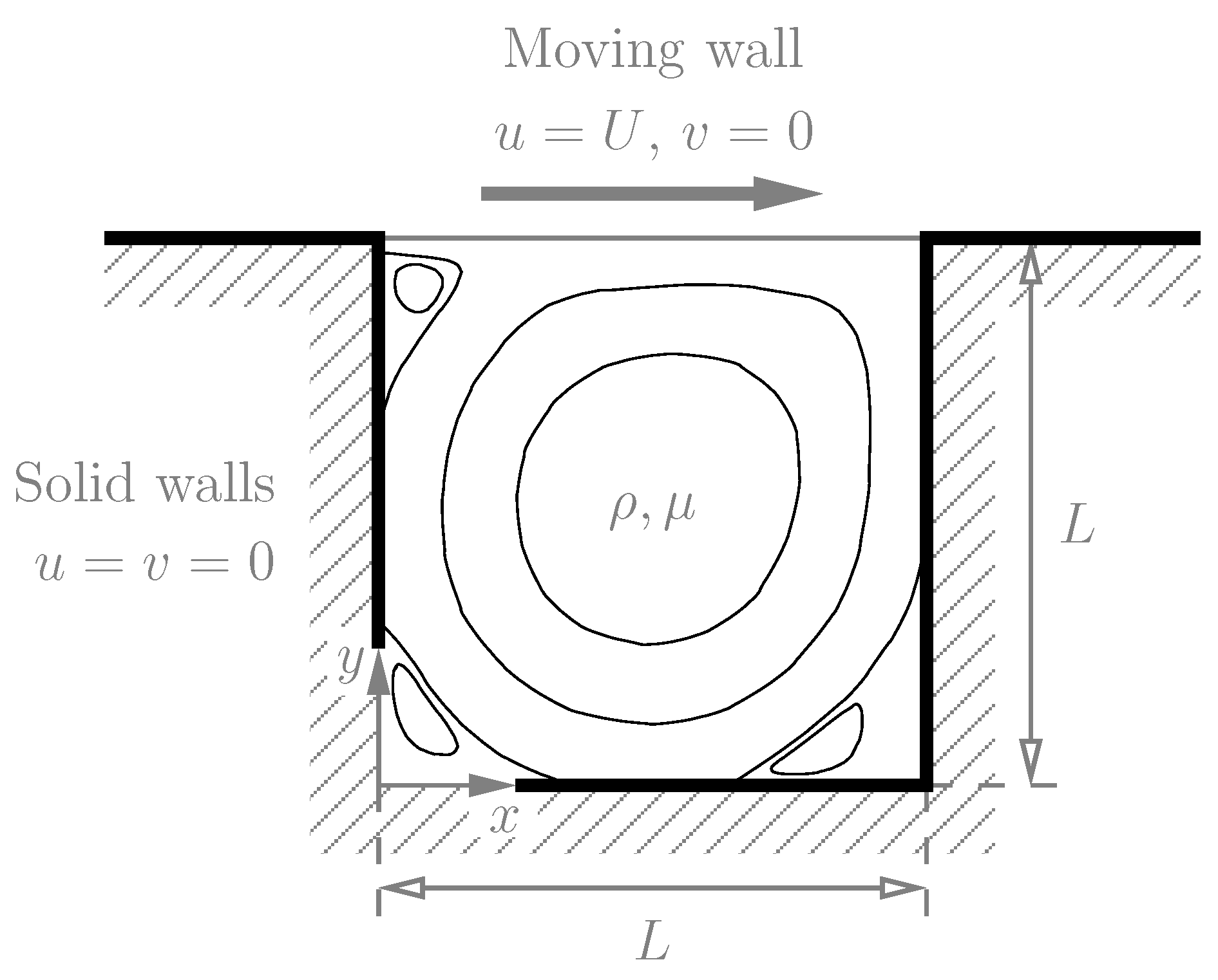
The lid-driven cavity flow.This is a classical benchmark problem that has been widely used since the early days of CFD to assess and validate new techniques and methods. This test case is easy to set and simulate because its boundary conditions are particularly simple. However, the fully developed flow displays almost all fluid mechanical phenomena, with increasingly complex aspects emerging as the Reynolds number is increased, such as corner eddies, laminar to turbulence regime transition, and even turbulence at high Reynolds number. A recent comprehensive review of the literature on the subject can be found in [22], where the work of several authors is presented and discussed [23,24,25,26,27,28]. Available benchmark results have been tabulated to provide a comprehensive source of validation data [29].
(ii)
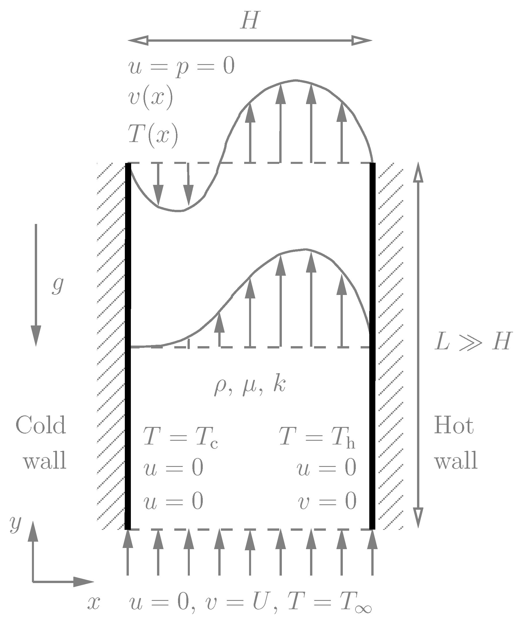
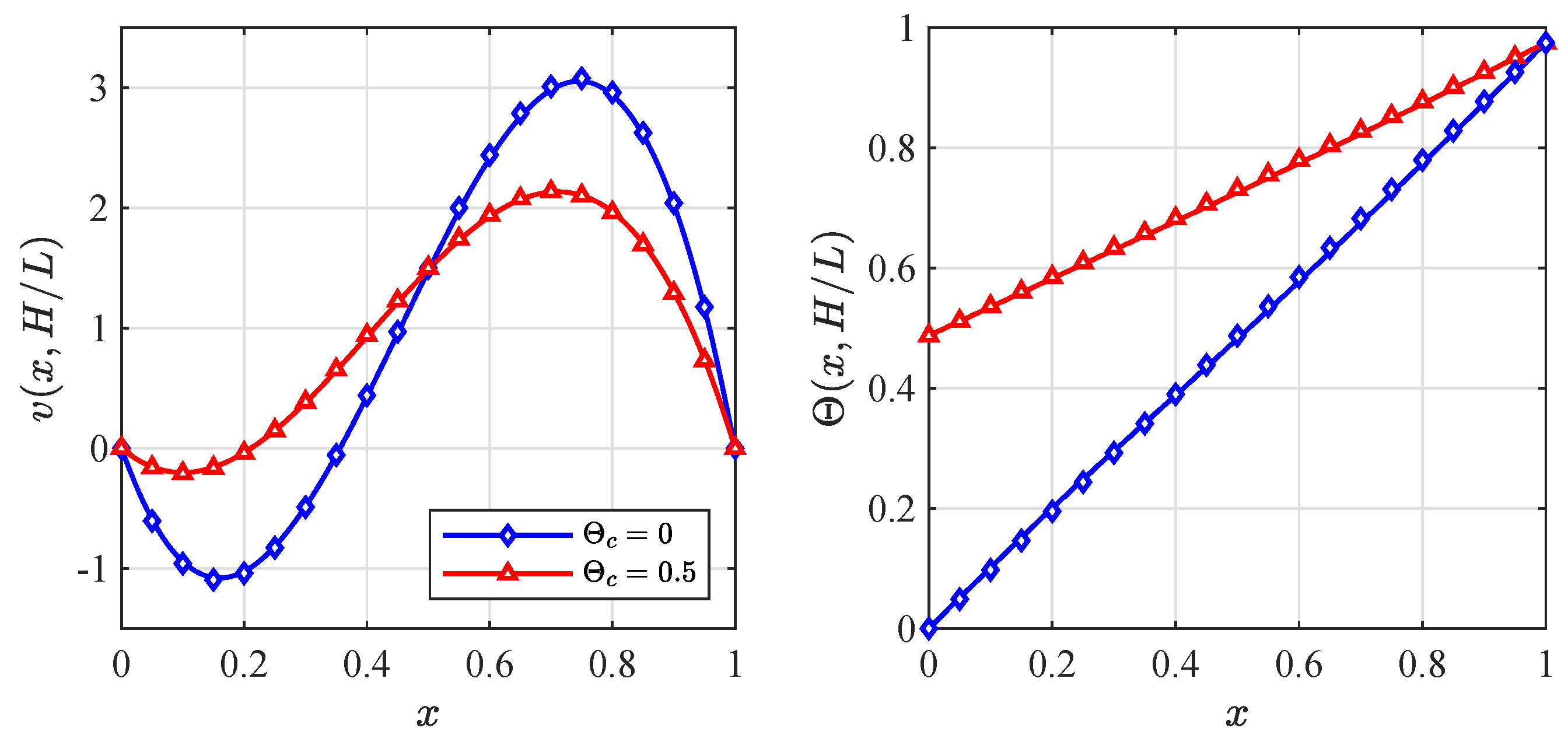
Mixed convection flow in a vertical channel with asymmetric wall temperatures. In this mixed convection heat transfer problem, an initially uniform flow develops in a slender vertical channel whose walls are at different temperatures. The cold and hot wall temperatures may also differ from the incoming flow temperature. As a result of the upward buoyancy force that appears near the hot wall, the velocity increases in the near-wall region. As the fluid accelerates downstream, the fluid near the cold wall may suffer flow reversal so as to maintain the imposed fixed flow rate. One of the most interesting features exhibited by this flow is thus the possibility of flow reversal at the cold wall as the flow develops. The occurrence (or not) of flow reversal depends on the length of the vertical channel and the buoyancy effect induced by the temperature difference between the hot and cold walls. Previous studies have shown that for the flow reversal to occur, in high Reynolds number flows the ratio of the Grashof number to the Reynolds number must be higher than a critical value that depends on the wall temperature difference ratio [30,31,32,33,34,35,36,37,38,39,40,41,42,43].
(iii)
Unsteady incompressible flow past a circular cylinder. The flow of a constant density fluid past a bluff body is another classical problem that has been widely studied in the literature. Understanding the flow regimes past bluff bodies poses a daunting challenge, so that 2D and 3D vortical structures in wakes of different bodies have been analyzed by scientists and engineers for decades. The reason for this interest is the vast range of applications of external flow past round bluff bodies: aerodynamics (planes, rockets, ground vehicles), hydrodynamics (ships, submarines) or wind energy (wind turbines), to name the few. At very low Reynolds numbers (creeping flow) the flow past a non-heated circular cylinder is symmetric in the streamwise direction [44,45,46,47]. As the Reynolds number grows to values of order unity the symmetry is lost, and when it exceeds a critical value the non-linear convective effects trigger the onset of steady flow separation, accompanied by the appearance of steady recirculation bubbles behind the cylinder. One important aspect of these flows is the so-called vortex shedding, which is an oscillating flow pattern that emerges for even larger Reynolds numbers. This regime has been thoroughly studied experimentally [48,49,50,51,52] and numerically [53,54,55,56,57]. The alternate shedding of vortices in the wake leads to the well known Kármán vortex street, which originates large fluctuating pressure forces in the direction transverse to the flow and may cause structural vibrations, acoustic noise, or resonance, which in some cases may lead to structural damage or even collapse.
(iv)
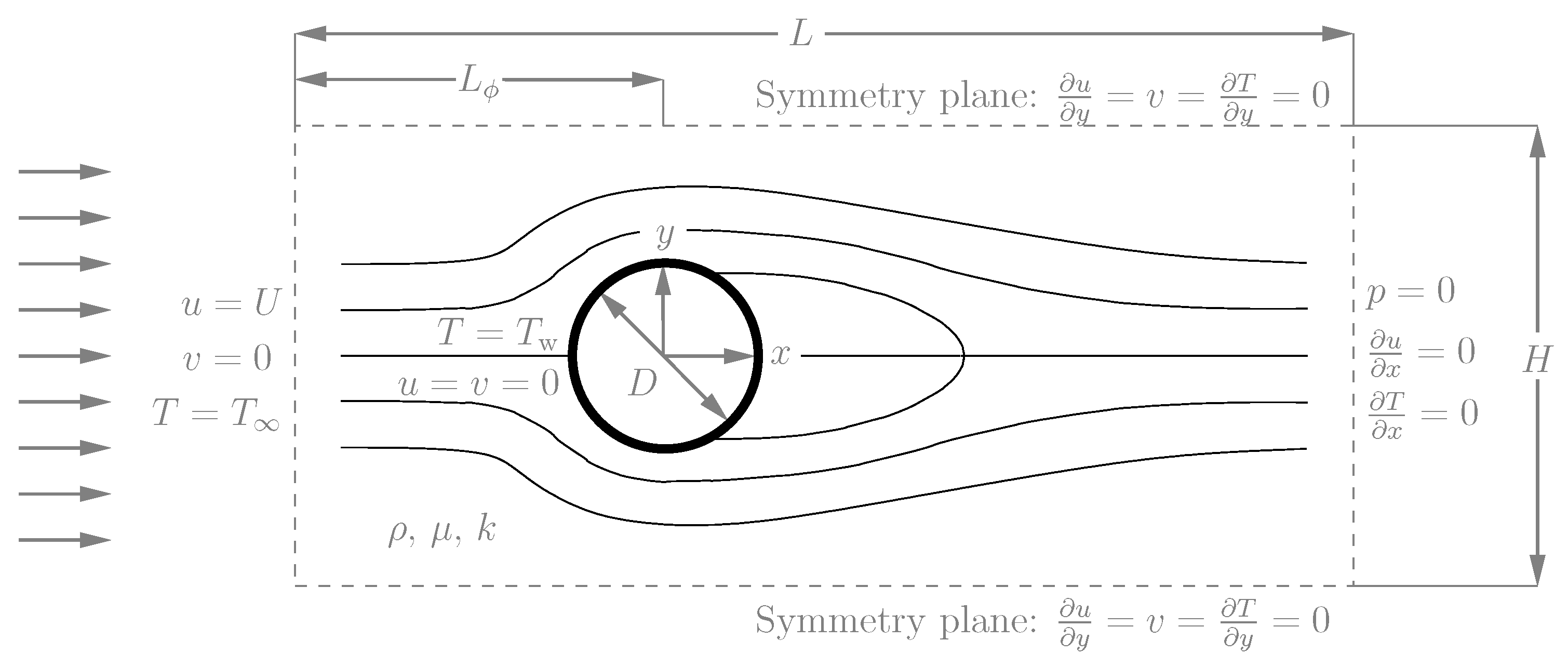
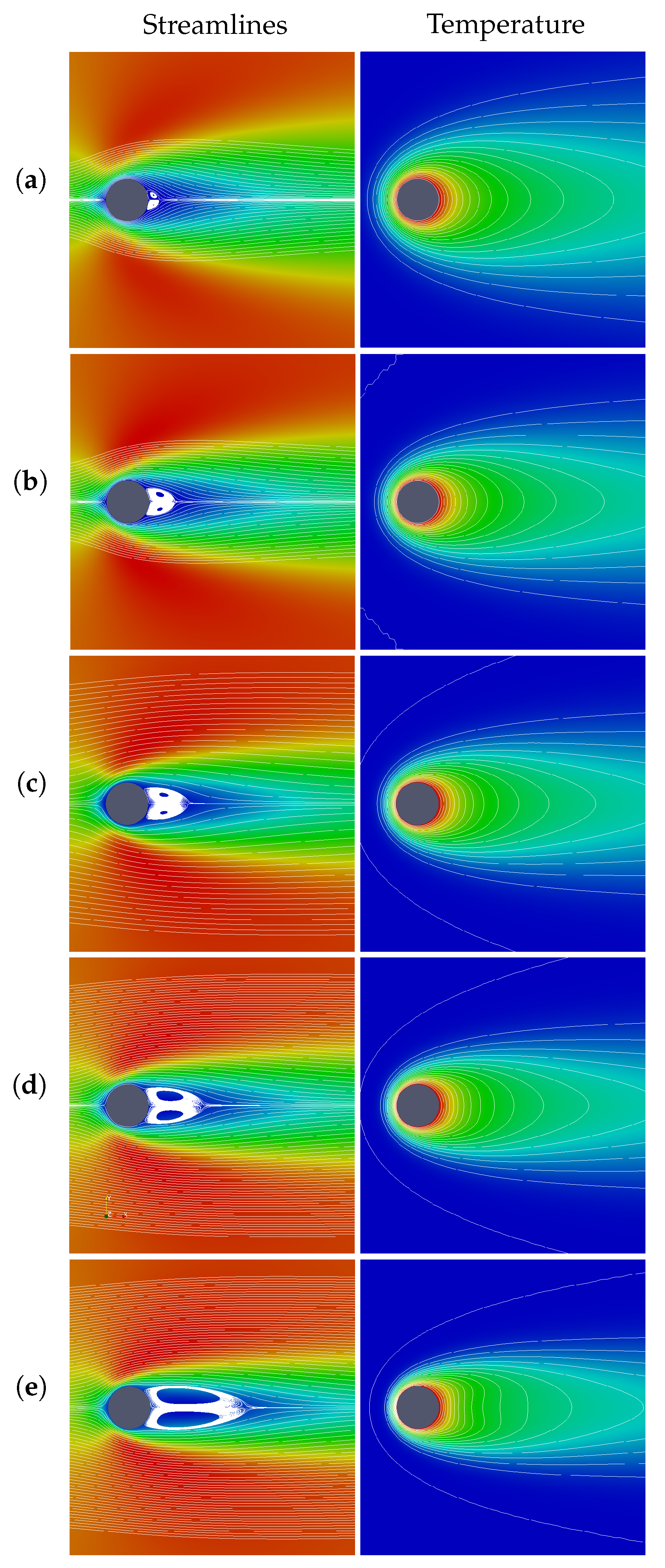
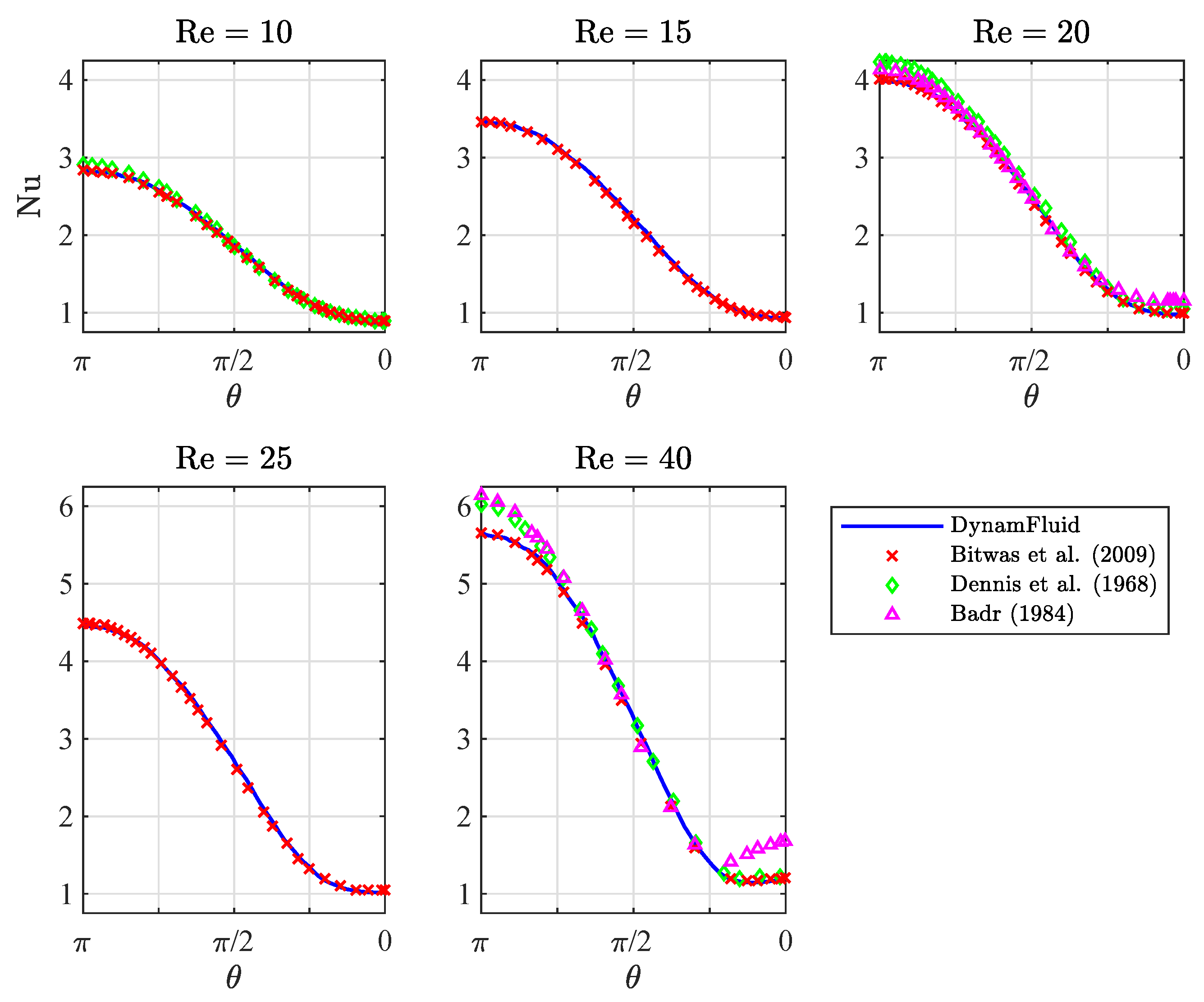
Steady non-isothermal flow past a circular cylinder with negligible buoyancy effects. This case is similar to the previous one but with the particularity that the temperature of the cylinder differs from the temperature of the incoming fluid, which causes the flow past a circular cylinder to exhibit interesting heat transfer features. This problem is of interest for the design of cylinder-shaped sensors located in fluid streams, hot-wire anemometers, tube heat exchangers, nuclear reactor fuel rods and chimneys. In this work, attention will be restricted to steady flow with negligible buoyancy effects, with the aim of characterizing the local Nusselt number at the cylinder wall for different Reynolds numbers [44,54,58,59].

2. Governing Equations

Let x = ( x , y , z ) T Ω t R 3 be the spatial domain at time t ( 0 , T ) , with x i denoting the i-th cartesian coordinate. Using the Einstein summation convention, the governing equations for three-dimensional unsteady flow with variable density (due, e.g., to temperature variations) can be written as follows
ρ t + ( ρ u j ) x j = 0
( ρ u i ) t + ( ρ u j u i ) x j = p x i + τ i j x j + ρ g i , i = { 1 , 2 , 3 }
( ρ e T ) t + ( ρ u j e T ) x j = ( p u j ) x j + ( τ i j u i ) x j + ρ g j u j + x j k T x j ,
where ρ is the fluid density, u i the i-th component of the velocity vector u = ( u , v , w ) T , e T = e + u i u i / 2 the total energy per unit mass (with e = c v T the specific internal energy per unit mass, assuming a calorically perfect fluid), p the pressure, T the absolute temperature, g i the i-th component of the acceleration of gravity, and k the thermal conductivity. In the above equations τ i j represent the deviatoric stress components
τ i j = μ u i x j + u j x i 2 3 δ i j u k x k ,
where μ is the dynamic viscosity and δ i j the Kronecker delta.
In non-isothermal flows where the density variations are small but the flow is driven by buoyancy forces, such as in natural or mixed convection problems, one may simplify the equations by means of the Boussinesq approximation. This approximation assumes that variations in density have no effect on the flow field other than to give rise to buoyancy forces. In this case, the continuity and momentum equations take the simplified form
u j x j = 0
ρ u i t + ( u j u i ) x j = p x i + τ i j x j + ρ ( 1 β ( T T ) ) g i , i = { 1 , 2 , 3 }
where ρ is the reference fluid density, T the reference temperature, and β = ρ 1 ( ρ / T ) p the thermal expansion coefficient.
In the Boussinesq approximation, the energy equation is often simplified by also ignoring the density variations. However, in this work, the energy equation will be kept in its general form, without any further simplification. The reason for this approach is to minimize the approximation error when computing the temperature field in a fluid that undergoes tiny variations of density, and to give a unified treatment to the energy equation independently of the way density is computed. In the range of Reynolds number considered here, the different treatments of the energy equation, and the assumption of constant specific heats, do not make a significant difference. Leaving the general form allows validating the implementation of the energy equation when the Boussinesq approximation is used in the Navier–Stokes equations but not in the energy equation.
Let L be the characteristic length, U the characteristic velocity, L / U the characteristic residence time of the problem, ρ the reference density, μ the reference dynamic viscosity, and k the reference thermal conductivity. With these scales, the following dimensionless variables can be introduced
x i * = x i L , t * = U t L , ρ * = ρ ρ , u i * = u i U , p * = p p ρ U 2 , τ i j * = τ i j L μ U , g i * = g i g , μ * = μ μ , e T * = e T U 2 , T * = c p T U 2 , k * = k k
where p represents a convenient pressure datum, and g 9.81 m / s 2 is the acceleration of gravity.
The asterisk will be dropped in the following for simplicity, so that all variables will be assumed to be non-dimensional. Thus, the general governing Equations (1)–(3) can be rewritten as follows
ρ t + ( ρ u j ) x j = 0
( ρ u i ) t + ( ρ u j u i ) x j = p x i + 1 Re τ i j x j + 1 Fr ρ g i , i = { 1 , 2 , 3 }
( ρ e T ) t + ( ρ u j e T ) x j = ( p u j ) x j + 1 Re ( τ i j u j ) x i + 1 Fr ρ g j u j + 1 Re Pr x j k T x j ,
where Re = ρ U L / μ is the Reynolds number, Fr = U 2 / ( L g ) is the Froude number, and Pr = μ c p / k is the Prandtl number, defined in terms of the specific heat at constant pressure c p , assumed here to be constant. Note that for liquids both specific heats are equal c p = c v , whereas for gases c p = c v + R g , where R g = R / W is the gas constant, defined as the ratio between the universal gas constant R = 8.314 J / ( mol · K ) and the molecular mass of the gas W that is constant for gases of uniform composition.
Under the Boussinesq approximation, it is convenient to define the normalized dimensionless temperature
Θ = T T T w T ,
in terms of the reference temperature T and a characteristic temperature T w (e.g., that of a hot or cold wall, thereby the subscript w) that determines the characteristic temperature difference of the problem, T w T . In this case, the momentum conservation Equation (6) and the energy conservation Equation (3) can be rewritten as follows, where the asterisks are dropped again so that all variables are non-dimensional
u i t + ( u j u i ) x j = p x i + 1 Re τ i j x j + 1 Fr g i Gr Re 2 g i Θ , i = { 1 , 2 , 3 }
ρ e T t + ( u j e T ) x j = ( p u j ) x j + 1 Re ( τ i j u j ) x i + 1 Fr ρ g j u j + 1 Re Pr x j k T x j ,
while the continuity Equation (5) remains unchanged, implying the divergence-free nature of the velocity field. The simplified form of the continuity equation has been used, in particular, to rewrite the convective term in the energy Equation (13) including the velocity u j into the spatial derivative. Note that, following standard practice, in the momentum conservation Equation (12) the dimensionless density has been assumed to be constant ( ρ = 1 ) except in the buoyancy term, which is written in terms of the Grashof number
Gr = β g ( T w T ) L 3 ν 2 ,
and the normalized dimensionless temperature Θ , given by (11) in terms of the dimensionless temperature T computed from (13).
Finally, to be well posed, the mathematical problem also requires appropriate boundary conditions and a set of initial conditions for all the variables to be solved.

3. Numerical Method

3.1. Temporal Discretization: The Characteristics-Based-Split Algorithm

Following Zienkiewicz’s et al. [60,61,62,63,64], the Navier-Stokes equations can be sampled in time using a characteristic method, the so-called characteristic-based-split (CBS) scheme. To obtain the numerical solution, the time interval will be divided into N t subintervals I n : = ( t n , t n + 1 ] with constant time step size Δ t = t n + 1 t n . Then, a variable ϕ at time n + θ can be approximated as ϕ n + θ = ( 1 θ ) ϕ n + θ ϕ n + 1 , where the superscript denotes the time at which the variable is evaluated. As a result, it can be written that
ϕ n + θ = ( 1 θ ) ϕ n + θ ϕ n + 1 = ϕ n + θ Δ ϕ ,
with Δ ϕ = ϕ n + 1 ϕ n .
Consequently, the CBS scheme, proposed by Zienkiewicz and Codina [61], applied to the governing Equations (1), (12) and (13) can be sampled in time as follows
u i n + 1 u i n Δ t = Δ u i Δ t = ( u j u i ) x j + 1 Re τ i j x j + 1 Fr g i Gr Re 2 g i Θ n p n + θ 2 x i , i = { 1 , 2 , 3 }
ρ n + 1 ρ n Δ t = Δ ρ Δ t = 1 a 2 n Δ p Δ t = ρ u j n + θ 1 x j
ρ n e T n + 1 e T n Δ t = ρ n Δ e T Δ t = ρ ( u j e T ) x j ( p u j ) x j + 1 Re ( τ i j u j ) x i + 1 Fr ρ g j u j + 1 Re Pr x j k T x j n
where the continuity equation for incompressible fluids has been substituted by an equation of conservation of mass (17) that includes an artificial compressibility [65]. In that equation a represents the speed of sound in the fluid, which in the incompressible limit tends to infinity. The principal asset of this split algorithm is that it does not only apply to compressible flows, but also to incompressible flows, which makes it suitable for a wide variety of applications. In the above equations, θ 1 and θ 2 represent, respectively, the velocity and pressure relaxation factors. The explicit form of the algorithm is θ 2 = 0 , whereas in the semi-implicit form θ 2 [ 0.5 , 1 ] . In both cases the value of θ 1 [ 0.5 , 1 ] . In the numerical simulations presented in this paper we have considered the semi-implicit algorithm, setting the velocity relaxation factor to θ 1 = 1.0 , and the pressure relaxation factor to θ 2 = 1.0 . For this parameter choice, second-order accuracy in time is expected [61]. Moreover, the algorithm imposes a restriction to the time step size Δ t and it is conditionally stable, as reported by [61]. In its semi-implicit form [66], the time step size must be Δ t min { h / | u i | , h 2 / ( 2 ν ) } , whereas in the explicit form, Δ t h / | a | , leading to a more stringent time step in incompressible fluids. That is the reason why, for incompressible fluids, the semi-implicit form is cheaper in terms of computational cost, providing the required results in less time.
Equation (16) is coupled to Equation (17) and for this reason it cannot be used explicitly. To overcome this limitation, an auxiliary variable Δ u * * is introduced, defined by
Δ u i * * = u i * * u i n = Δ t [ ( u j u i ) x j + 1 Re τ i j x j + 1 Fr g i Gr Re 2 g i Θ + Δ t 2 u k x k ( u j u i ) x j 1 Fr g i + Gr Re 2 g i Θ ] n .
This equation does not contain the pressure term and the variable u i * * can thus be computed explicitly. When the pressure term is available, the following correction is applied
Δ u i = u i n + 1 u i n = Δ u i * * Δ t p n + θ 2 x i Δ t 2 2 u k x k p n + θ 2 x i .
Expressing Δ u i n + 1 as a function of Δ u i * * using (20) and substituting the result in (17) yields
Δ ρ = 1 a 2 n Δ p = Δ t u i n x i + θ 1 Δ u i * * x i Δ t θ 1 2 p n x i x i + θ 2 2 Δ p x i x i .
Finally, expressing Δ e T as a function of e T n gives
ρ Δ e T = Δ t [ ( u j ( ρ e T + p ) ) x j + 1 Re ( τ i j u j ) x i + 1 Fr ρ g j u j + 1 Re Pr x j k T x j + Δ t 2 u j x j ( u i ( ρ e T + p ) ) x i ] n .
The way the variables of the problem are solved is summarized in the following step sequence:
  • Calculate Δ u i * * from Equation (19).
  • Calculate Δ ρ or Δ p from Equation (21).
  • Calculate Δ u i from Equation (20), which yields the velocity at time t n + 1 .
  • Calculate Δ e from Equation (22), which can be calculated in parallel with the other steps since the right hand side of Equation (22) does not depend on the variables at time t n + 1 . Step 4 allows obtaining the value of the energy at time t n + 1 .
The reason for choosing the CBS algorithm instead of others is to achieve second order convergence in both time and space using linear finite elements (TRIA and/or QUAD). Additionally, since the right hand side of the different equations of the algorithm are treated explicitly, they are easy to parallelize, as it has been done in the implementation of the algorithm.

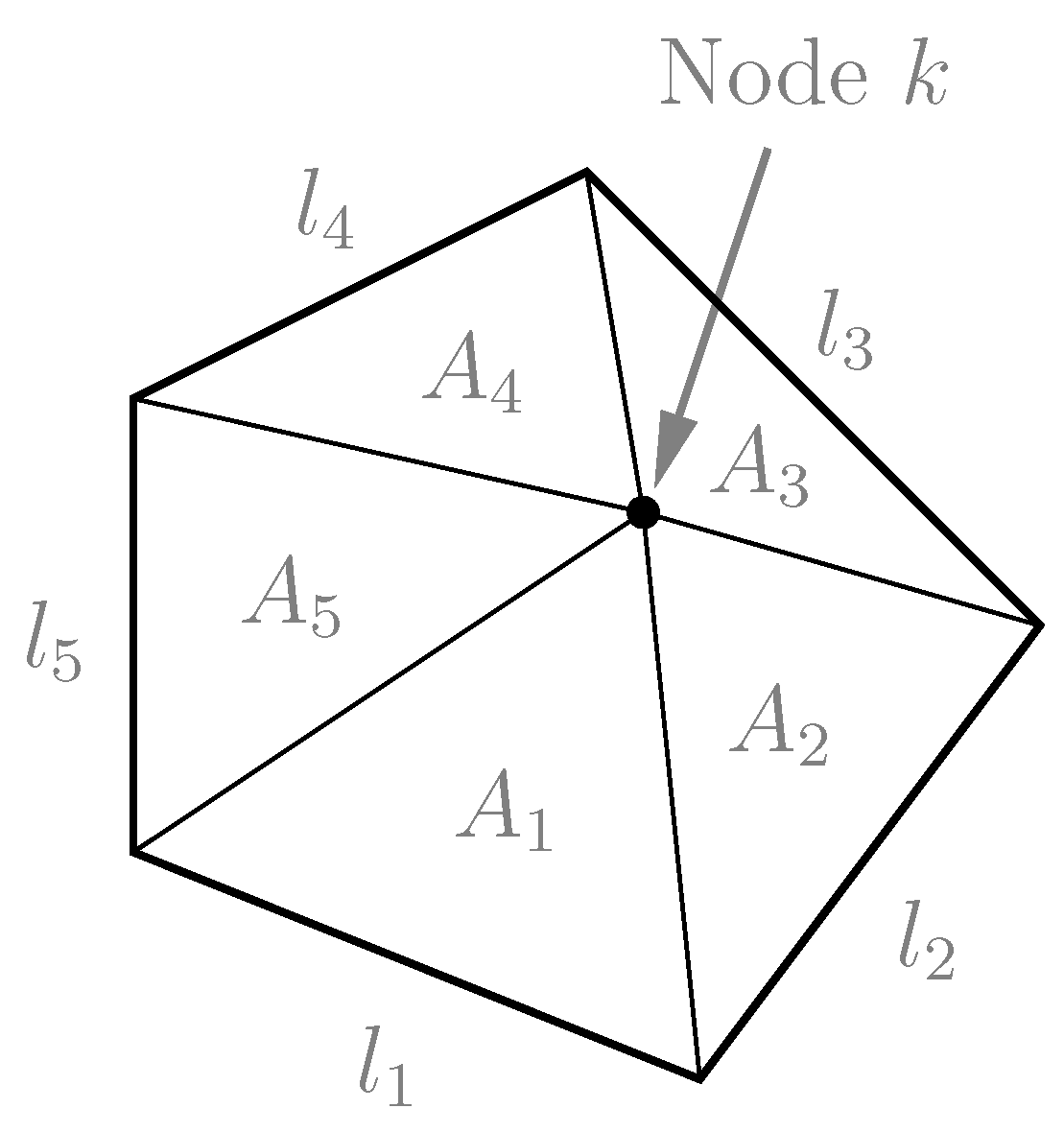
3.2. Spatial Discretization

Following the characteristics-Galerkin approximation, Equations (19)–(22) are discretized in space using the finite element method [67,68,69]. To this end, the spatial domain is divided into a regular, unstructured triangulation T h of non-overlapping elements. Associated with that triangulation, a conforming finite element space V h is defined composed of continuous, piecewise polynomials over each mesh element. The current implementation of the software uses only linear polynomials for all fluid variables, so higher order elements are not considered. Therefore, the numerical method is expected to be second order in space for smooth solutions in the L 2 -norm. The advantage of the finite element method, as spatial discretization method, is that it allows to work with complex geometries, and to use fine or coarse finite elements in different zones of the domain (local mesh refinement) [70]. Moreover, the implemented code supports both TRIA and QUAD finite elements.
Hence, if m is the number of mesh points (or nodal points) of the triangulation T h , the numerical solution ϕ h belonging to the finite element space V h can be written as
ϕ h = k = 1 m N h k ϕ k ,
where the summation spans over the set of nodes comprising the sampled domain, being k the index of the node, for 1 k m . ϕ k is the unknown variable evaluated at node k, and { N h k } k = 1 m is the set of basis functions of V h satisfying N h k ( x j ) = δ k j , with δ k j the Kronecker delta. Moreover, Equation (23) may be expressed in matricial form as
ϕ h = N h ϕ ¯
with
ϕ ¯ = ϕ 1 , , ϕ k , , ϕ m T and N h = N h 1 , , N h k , , N h m .
In this problem the generic variable ϕ h will be replaced by the unknown fluid variables: the pressure, p, the velocity components, u i , the total energy, ρ e T , and the temperature, T.
As a final step to apply the standard Galerkin approximation via the Finite Element method, the weak formulation of Equations (19)–(22) must be obtained. Thus, equations can be weighted and integrated over the sampled domain using the basis functions N h ϕ k V h 0 ϕ , where V h 0 ϕ is the finite element space of functions that take null values in the dirichlet boundary associated with the variable ϕ h = { u i , p , T } (which means that it does not include the basis functions associated with the dirichlet nodes, whose values for the variable ϕ h are known).
The weak formulation of Equation (19) (Step 1 of the algorithm to compute Δ u i * * for i = { 1 , 2 , 3 } ) in the standard Galerkin approximation is the following
Ω N h k Δ u i * * d Ω = Δ t Ω N h k ( u j u i ) x j d Ω 1 Re Ω N h k x j τ i j d Ω Ω N h k Gr Re 2 g i Θ 1 Fr g i d Ω n + Δ t 1 Re Γ N h k τ i j n j d Γ n Δ t 2 2 Ω x j ( u j N h k ) Gr Re 2 g i Θ 1 Fr g i + ( u j u i ) x j d Ω n ,
where n j denotes the j-th component of the unit outward normal vector to the boundary surface and N h k V h , since it does not impose dirichlet boundary condition over Δ u i * * .
To obtain the weak formulation of Equation (21) (Step 2 of the algorithm to compute Δ p = p n + 1 p n ), the equation should be multiplied by the N h p k basis functions not associated with the dirichlet boundary nodes where pressure is prescribed p = p ˜ n + 1 at Γ p . This gives
Ω N h p k Δ ρ d Ω = Ω N h p k 1 a 2 Δ p d Ω = Δ t Ω N h p k x j u j n + θ 1 Δ u j * * θ 1 Δ t p n x j θ 1 θ 2 Δ t Δ p x j d Ω Δ t Γ p Γ N h p k u j n + θ 1 Δ u j * * θ 1 Δ t p n x j θ 1 θ 2 Δ t Δ p x j n j d Γ ,
where the boundary Γ p Γ is the entire boundary of the domain minus the dirichlet pressure boundary. In the computation of the boundary integral on Γ p Γ , the Dirichlet condition for the velocity component, u i , may also be specified, in which case, the integrand will match the prescribed velocity, u i n + θ 1 Δ u i * * θ 1 Δ t p n / x i θ 1 θ 2 Δ t Δ p / x i = u ˜ i , at Γ u .
In the same way, to build the weak formulation of Equation (20) (Step 3 of the algorithm to compute Δ u i = u i n + 1 u i n for i = { 1 , 2 , 3 } ), the basis functions N h u k not associated with the dirichlet boundary nodes where velocity is prescribed, u i n + 1 = u ˜ i at Γ u , must be considered. This results in
Ω N h u k Δ u i d Ω = Ω N h u k Δ u i * * d Ω Δ t Ω N h u k p n + θ 2 x i d Ω 1 2 Δ t 2 Ω ( u j n N h u k ) x j p n x i d Ω
Finally, the weak formulation of the energy conservation Equation (22) (Step 4 of the algorithm to compute T n + 1 through Δ e T = e T n + 1 e T n ) takes the form
Ω N h T k ρ Δ e T d Ω = Δ t Ω N h T k x j u j ρ e T + p d Ω 1 Re Ω N h T k x j τ i j u j + 1 Pr k T x j d Ω + Ω N h T k 1 Fr ρ g j u j d Ω n + Δ t 2 2 Ω x j u j N h T k x j u j ρ e T + p d Ω n + Δ t 1 Re Γ T Γ N h T k τ i j u j + 1 Pr k h x i n i d Γ n ,
where N h T k are the basis functions not associated with the dirichlet boundary nodes where temperature (energy) is prescribed, T n + 1 = T ˜ at Γ T . Moreover, in the computation of the boundary integral on Γ T Γ , the value of the temperature gradient (heat flux) can be specified on some part of it (neumann boundary) as boundary condition.

4. Software Validation

In order to validate the implementation of the CBS algorithm described above, four test cases have been selected for study. Although the implementation of DynamFluid allows the integration of the Navier–Stokes equations in their general form (1)–(3), it can also be applied to fluid dynamics problems within the Boussinesq approximation (5) and (6). This is the approach chosen for the validation with the test cases presented in this section. All simulations are two-dimensional, hence we shall restrict our attention to cases with x i = ( x , y ) T , u i = ( u , v ) T , and g i = ( g x , g y ) T . As discussed in the numerical section, in all test cases the velocity and pressure relaxation factors θ 1 and θ 2 have been set to unity
.

4.1. Lid-Driven Cavity Flow

The first step in the validation of a new CFD tool is to check if it is able to predict the flow behaviour in confined domains with simple boundary conditions. The flow in a cavity with an upper mobile lid, shown schematically in Figure 1, is considered as a standard software validation case for steady incompressible flows in confined geometries. In the lid-driven cavity, the fluid is confined in a 2D square cavity of side length L ( L ) , with a zero velocity enforced by the no-slip condition in all the walls of the square cavity except in the top wall, where a uniform slip velocity U ( U ) is imposed. Additional parameters of the problem include the density, ρ ( ρ ) , and viscosity, μ ( μ ) , of the fluid, assumed here to be constant. Under isothermal conditions, the only governing parameter is the Reynolds number Re = U L / ν , based on the lid velocity, the side length of the squared cavity, and the kinematic viscosity of the fluid, ν = μ / ρ ( ν ) .

4.1.1. Literature Review

The lid-driven cavity flow has been extensively addressed by many authors [23,24,25,26,27,28]. Erturk et al. [23] performed numerical calculations of the two-dimensional steady incompressible lid-driven cavity flow for Reynolds number up to 21,000 with an extremely small residual error of the steady solution, finding a fourth vortex at the bottom left corner and a third vortex at the top left corner as the Reynolds number was increased, and obtaining a solution free of spurious oscillations despite the high Reynolds number.
Erturk [24] studied in detail the two-dimensional lid-driven cavity flow considering all physical, mathematical and numerical aspects, concluding that physically this flow is not two-dimensional but three-dimensional above a certain Reynolds number when the two-dimensional solution becomes unstable to small three-dimensional perturbations. Thus, while numerical solutions for the planar lid-driven cavity flow for high Reynolds numbers can be obtained, this flow can be considered fictitious. One important point for obtaining a solution at high Reynolds number is that a sufficiently fine mesh is needed so as to rule out any spurious oscillatory solution provided by the numerical method that prevents reaching the steady-state solution.
Yapici et al. [25] managed to perform several simulations up to Reynolds number 65,000, obtaining a steady solution with two new vortices in the bottom left and right corners of the square cavity for Reynolds number larger than 25,000.
Erturk et al. [29] also studied the benchmark problem of a driven skewed cavity flow for skew angles of 30 and 45 . Using a very fine grid and highly accurate numerical solvers, they obtained numerical results for Reynolds number varying from 100 to 1000.

4.1.2. Boundary and Initial Conditions

In dimensionless form, a unit horizontal velocity is imposed at the upper wall, u 1 = v = 0 , whereas the non-slip condition is imposed at the left, bottom and right walls, u = v = 0 . As an initial condition, both components of the velocity are set to 0 in all the points of the domain, except at the upper wall (lid) where the horizontal component is set to 1. The pressure is arbitrarily set to zero, p = 0 , at the lower-left corner of the cavity.

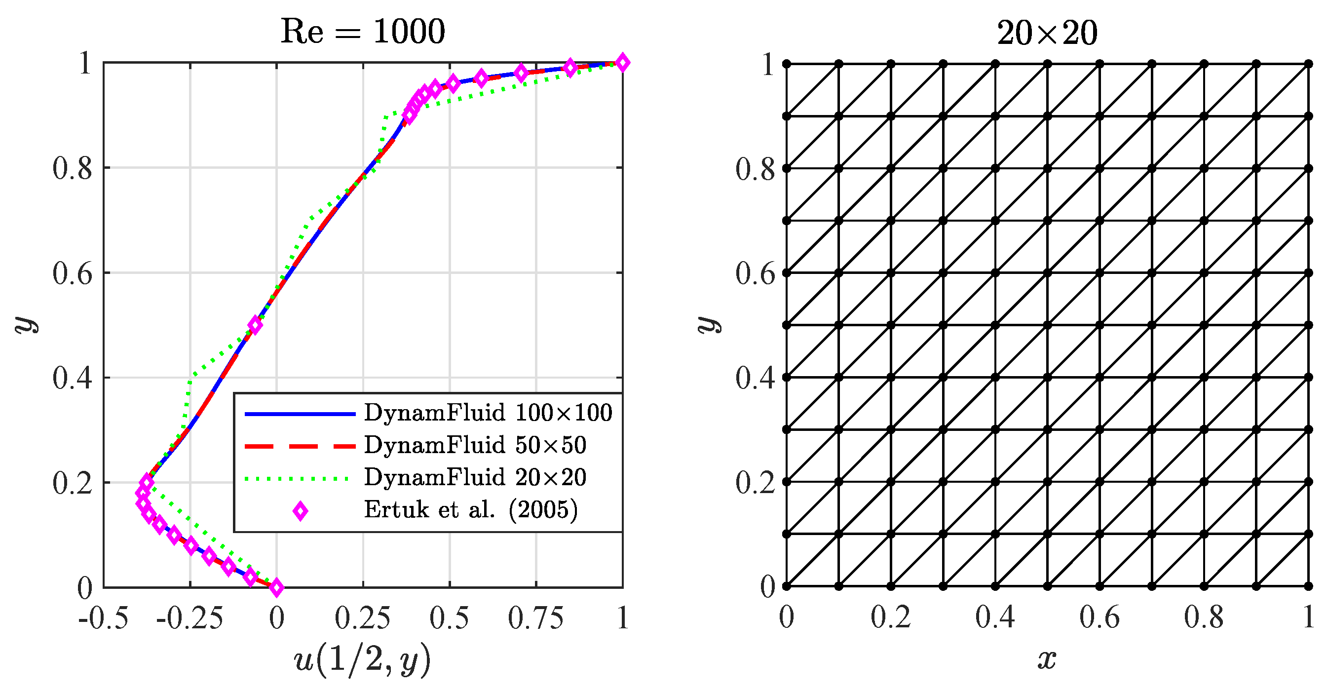
4.1.3. Convergence Analysis
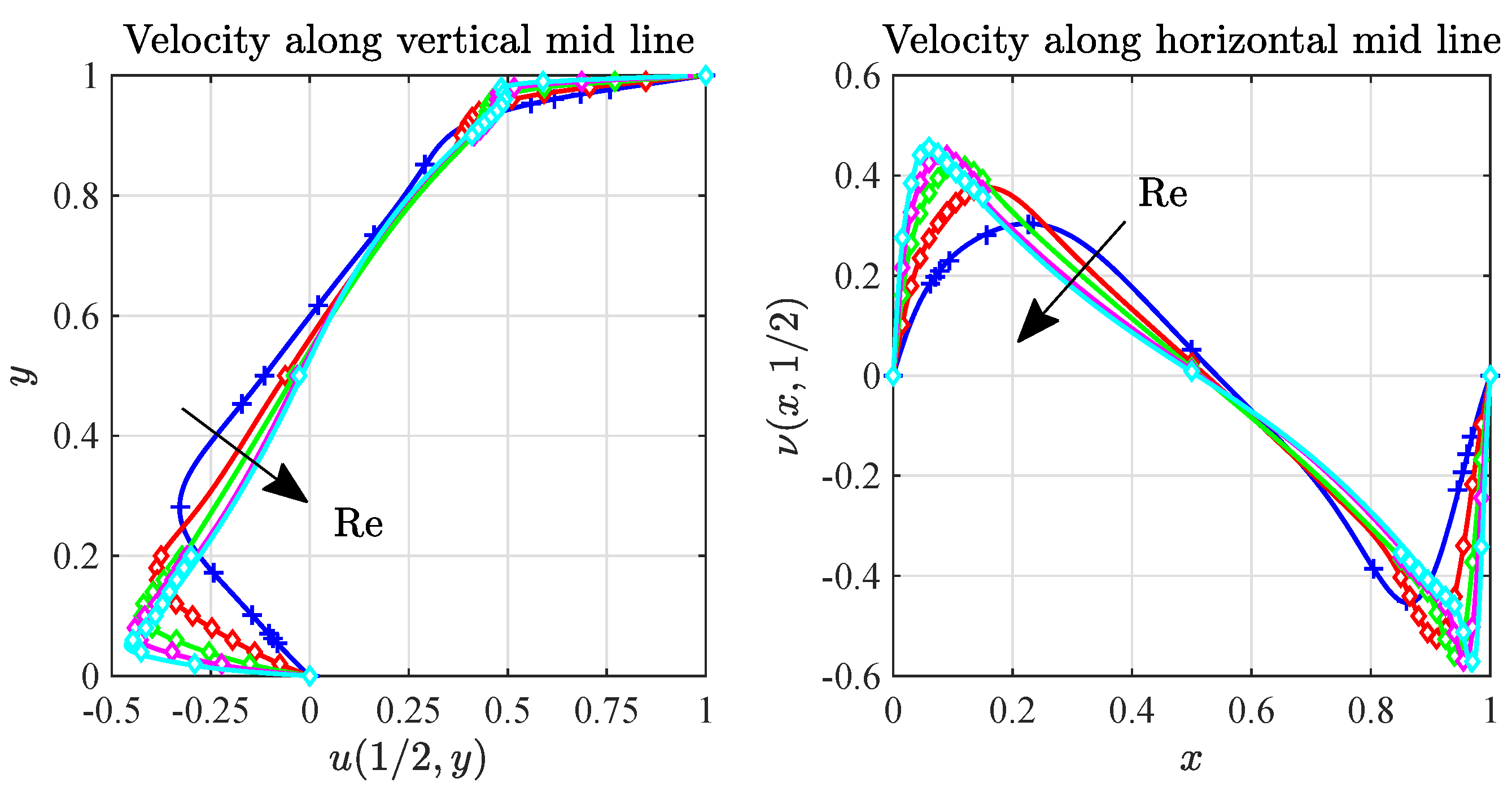
In this section, we study the influence of the mesh in the numerical solution, which includes analyzing the influence of the mesh space discretization and cell size in the convergence of the solution. The method for estimating the convergence order of an algorithm requires to obtain a solution for different meshes with different element sizes. The meshes used for the convergence analysis are three uniform (i.e., equispaced) meshes using TRIA elements for the discretization of the domain with (mesh #1) 20 × 20 , (mesh #2) 50 × 50 and (mesh #3) 100 × 100 points, respectively. The coarser mesh is shown in Figure 2 for illustrative purposes.
The boundary conditions are applied to the mesh assuming the ramp condition: the velocity in the top of the cavity (moving lid) grows from zero in the corners of the cavity (left and right) until the non-dimensional value in the span of a cell/element. Alternatively, other researchers use the leaking lid formulation, where the velocity in the top lid is constant and equal to the imposed velocity and zero in the rest of the walls.
The Reynolds number used for showing the influence of the mesh element size in the accuracy of the solution is Re = 1000 . The variable chosen for the convergence analysis is the horizontal velocity component u along the vertical line that goes through the center of the cavity. The steady-state solution is obtained by means of a transient simulation. It is assumed that the steady-state is reached when the relative value of the horizontal velocity in two successive time steps differ less than 10 9 , that is, k = 1 N | u k n + 1 u k n | / | u k n | 10 9 , the sum going through all N nodes in the mesh for the horizontal velocity component. Figure 2 shows that as the mesh is refined the solution tends to that obtained by Erturk et al. [23]. There is no appreciable difference between the results obtained with the 50 × 50 point and 100 × 100 point meshes.
For a TRIA element mesh composed by two-dimensional elements, as the one shown in Figure 3, an equivalent length for node k can be defined according to h k = min ( 2 A j / l j ) , where j spans from 1 to the number of adjacent elements connected to node k, A j is the area of the j-th element adjacent to node k, and l i is the length of the opposite edge belonging to the j-th element adjacent to node k [71].
The convergence order of the algorithm has been estimated using the well-known grid convergence index calculation. Following Roache [72], the order of convergence for the algorithm is obtained solving the following equations iteratively for the three different meshes, starting from the coarse mesh #1 ( 20 × 20 ) to the more refined mesh #3 ( 100 × 100 )
p = ln E r 32 / E r 21 + q ( p ) ln r 21
q ( p ) = ln r 21 p s r 32 p s
s = sign ( E 32 / E 21 ) ,
where E r i j = u i u j and r i j = h i / h j , with u i the horizontal velocity at mesh i and u j the horizontal velocity at mesh j, and h i the equivalent length for mesh i and h j the equivalent length for mesh j. This is translated into E r 32 being the difference in the estimating function between mesh #3 ( 100 × 100 ) and mesh #2 ( 50 × 50 ), and E r 21 between mesh #2 ( 50 × 50 ) and mesh #1 ( 20 × 20 ). Similarly, r 32 is the mesh ratio between mesh #3 and mesh #2, and r 21 between mesh #2 and mesh #1.
The iterative process starts with an initial guess for q ( p ) , e.g., q ( p ) = 0 in this case. Using the value of q at a given iteration step, the value of p is calculated at the next iteration step. After a few iterations, the convergence order p is obtained. Table 1 shows the maximum norm of the error E r L = max | u i u j | ( p = 2.71 ), and the mean norm of the error E r L 1 = ( 1 / N ) i = 1 N | u i u j | ( p = 1.98 ) for the implementation of the CBS algorithm discussed here applied to the lid-driven cavity flow.

4.1.4. Results for Re up to 10,000

Figure 4 compares numerical integrations of the lid-driven cavity flow carried out with DynamFluid with those obtained by Erturk [24] and Ghia et al. [26] for Reynolds number up to 10,000. Erturk et al. [23] reported that a 257 × 257 mesh is needed in order to get a steady solution for Reynolds number up to 10,000, thus a refined mesh of 257 × 257 elements was used for the simulations. As it can be seen, the agreement with previous results is excellent for Re 10,000, showing a slightly better agreement at low Reynolds number than at high Reynolds number.

4.2. Mixed Convection Flow in a Vertical Channel with Asymmetric Wall Temperatures

This is a mixed convection heat transfer problem in which an initially uniform flow develops in a slender vertical channel whose walls are at different temperatures. The flow is assumed to be two dimensional. The cold wall temperature, T c , and hot wall temperature, T h ( T w ) , are also different from the incoming flow temperature, T , as illustrated in Figure 5. The parameters characterizing the flow are the channel width H ( L ) and length L H , the cold and hot wall temperature differences, T c T and T h T , and the uniform velocity of the fluid entering the rectangular channel, U ( U ) . Additional parameters include the density, ρ ( ρ ) , viscosity, μ ( μ ) , and thermal conductivity, k ( k ) , of the fluid. The non-dimensional numbers that emerge in this problem are the Reynolds number, Re = U H / ν , based on the inlet velocity and the channel width, the Grashof number, Gr = g β ( T h T ) H 3 / ν 2 , defined in terms of the channel width and the hot wall temperature difference, and the wall temperature difference ratio Θ c = ( T c T ) / ( T h T ) . The Prandtl number is assumed to be constant, Pr = 0.72 . As shown in Figure 5, the acceleration of gravity is assumed to point opposite to the direction of the incoming flow. When the height of the channel is large compared to the channel width, the flow becomes fully developed far downstream, where the streamlines are parallel to each other and point vertically upwards.

4.2.1. Literature Review

The mixed convection flow in a vertical channel has been investigated by several authors. In a series of papers, Aung and Worku [30,31,32] studied the effects of buoyancy on the laminar vertical upward flow between parallel plates subject to two types of boundary conditions: (i) uniform wall temperatures, where the vertical walls may be at equal or different temperatures, and (ii) uniform heat fluxes, where the vertical walls may be subject to the same or different heat fluxes. They used the boundary layer approximation for their analysis when the dimensionless buoyancy parameter becomes Gr / Re instead of Gr / Re 2 . As a result, the controlling parameters are Gr / Re , the wall temperature difference ratio Θ c , and the Prandtl number, Pr = 0.72 , assumed to be constant. Aung and Worku [30] considered a set of values of Gr / Re in the range 0 , 25 , 50 , 100 and 250, founding that buoyancy extends the hydrodynamic entry length whereas it reduces the thermal entry length. As a general rule, no flow reversal was observed for sufficiently small values of Gr / Re , while it appeared for small values of Θ c and large values of Gr / Re (the larger value of Gr / Re , the larger the downwards velocity in the flow reversal region). Aung and Worku [31] predicted that with constant heat fluxes the ratio Gr / Re for flow reversal to happen is higher than with constant wall temperatures. In particular, for values of Gr / Re up to 500 no flow reversal was observed when uniform heat flux boundary conditions are used. Flow reversal did not occur either for symmetrically heated walls. As part of their study, they developed an analytical theory [32] for fully developed mixed convection flow including flow reversal, obtaining analytical expressions for the velocity profile and the temperature profile that will be used below for validation purposes.
Ingham et al. [40] found that infinite duct walls also bring about flow reversal in the vicinity of the cold wall, while Ingham et al. [41] obtained numerical solutions of the problem for a steady laminar mixed convection flow in a vertical duct with parallel plates. They compared this flow with the case of pure forced convection finding that large values of Gr/Re cause reverse flow in the channel (similar to Aung and Worku [30,32]). Kim et al. [43] used an implicit finite difference scheme to solve the governing equations in the conjugate heat transfer flow established between two vertical plates subject to asymmetric wall temperatures. They found that the independent parameters are the Grashof number, the Prandtl number, the solid to fluid thermal conductivity ratio, the wall thickness to channel width ratio, the channel height to channel width ratio and the asymmetric heating parameter.
Gau et al. [38] studied experimentally the heat transfer process in a vertical channel comprised of two parallel plates (one heated uniformly and the opposite wall insulated), having a very large buoyancy parameter Gr / Re 2 . From flow visualizations, they concluded that the reversal of the flow happened to be a V-shaped recirculating flow near the channel exit when Gr / Re 2 is greater than a critical value, although the reversal occurs initially downstream, but advances gradually downwards when Gr / Re 2 increases. El-Din [37], studied the flow development between two vertical plates with uniform heat and mass fluxes studying the effect of the thermal and mass transfer buoyancies. Cheng et al. [36] also studied this type of flow taking into account different boundary conditions (walls with constant temperature or with constant heat flux). Hamadah and Wirtz [39] investigated the effect of thermal buoyancy opposing the flow between two vertical plates with different boundary conditions (uniform asymmetric temperatures, uniform asymmetric heat fluxes, and the case of one wall at a uniform temperature and the other with uniform heat flux). Boulama and Galanis [35] provided analytical solutions for the fully-developed steady-state mixed convection flow past two vertical plates at constant temperatures and at constant heat flux (the two walls with the same type of boundary conditions or one with uniform temperature and the other with uniform heat flux).
Barletta et al. [34] studied the problem of a fully developed mixed convection flow with frictional heat generation in a vertical channel bounded by isothermal plane walls having the same temperature. Barletta [33] carried out an study of a laminar and fully developed flow with mixed convection in a rectangular and vertical duct where at least one of the two walls was isothermal, providing an analytical solution for the velocity and temperature fields. Desrayaud and Lauriat [73] investigated the flow reversal phenomena in a vertical channel with two parallel plates at symmetrically uniform heated walls when air is used as the fluid, for a laminar, mixed-convection flow with Reynolds number in the range 300 Re 1300 . The velocity and temperature profiles caused by the buoyancy forces were analyzed. Finally, Jeng et al. [42] investigated the mixed convection flow in a vertical channel with parallel walls at different temperatures: Θ c was in the range of 0 Θ c 1 , the Reynolds number was in the range of 1 Re 1000 , and the ratio Gr / Re in the range of 0 Gr / Re 500 . They found that when the streamwise coordinate was scaled out using the Reynolds number, the velocity and the temperature profile were independent of the Reynolds number for Re 50 .

4.2.2. Boundary and Initial Conditions

In the simulations presented below, the right wall is assumed to be at a higher temperature than the left wall, T h > T c . Two cases are considered in the study. In the first one the cold wall is at the same temperature than the incoming fluid, T c = T , or Θ c = 0 , and in the second case the cold wall is at a temperature halfway between the incoming fluid and the hot wall, T c T = 0.5 ( T h T ) , or Θ c = 0.5 . The dimensionless boundary condition for the velocity, pressure and normalized temperature are
  • Left, cold non-slip wall: u = v = Θ Θ c = 0 .
  • Right, hot non-slip wall: u = v = Θ 1 = 0 .
  • Bottom side, incoming flow: u = v 1 = Θ = 0 .
  • Top side, outgoing flow: p = u = v / y = θ / y = 0 .
Since the channel width is taken as length scale, the dimensionless width of the channel is one. By contrast, the dimensionless length of the channel is set to H / L = 80 1 , which is long enough to ensure that the flow is fully developed in the outflow boundary (see Figure 5 for details; note that the height and width are not to scale).

4.2.3. Discussion of Results

As previously discussed, Aung and Worku [32] obtained analytical expressions for the velocity profile and the temperature profile in the fully developed mixed convection flow established far downstream the channel, namely
v ( x ) = Gr Re ( 1 Θ c ) x 3 6 + x 2 4 x 12 6 x 2 + 6 x Θ ( x ) = x 0 < x < 1
the later corresponding to a linear temperature profile (i.e., a purely conductive heat flux) between the hot and cold walls. It is interesting to note that the analytical problem solved by Aung and Worku [30,31,32] included a simplified form of the energy equation that accounted only for thermal energy convection and heat conduction. As a consequence, the numerical results obtained with DynamFluid, which incorporates the general form of the energy Equation (10) or (13), can not be expected to match exactly the fully developed profiles given above.
Figure 6 shows the comparison between the fully developed profiles (33) with the numerical profiles predicted by DynamFluid in the outflow boundary corresponding to Re = 100 , Gr = 25,000, and two values of Θ c = { 0 , 0.5 } . In both cases the flow reversed near the cold wall ( x = 0 ) with higher downward velocities for Θ c = 0 , and the temperature profiles are very close to linear. The minor differences observed between the numerical and analytical predictions can be attributed to the differences in the treatment of the energy equation. In summary, the figure shows an excellent agreement between the numerical profiles and the analytical solution for both values of Θ c . This indicates that DynamFluid is able to predict accurately the velocity and temperature profiles in mixed convection problems under different conditions.

4.3. Isothermal Flow Past a Circular Cylinder

The flow past a circular cylinder is the prototypical benchmark case for the validation of external flows: either steady (the flow does not vary with time) or unsteady (the flow varies with time exhibiting either a transient or oscillatory behavior). Figure 7 shows an schematic representation of the flow: a circular cylinder of diameter D ( L ) surrounded by an unbounded fluid of density ρ ( ρ ) and viscosity μ ( μ ) with an uniform incoming velocity U ( U ) . In the non-isothermal flow past a circular cylinder, to be considered in the next section, the cylinder is assumed to be at a uniform temperature T w different from that of the incoming stream T . In both cases, the only non-dimensional parameter that appears in the limit of non-buoyant flows ( Ri = Gr / Re 2 0 ) to be considered here is the Reynolds number, Re = U D / ν , based on the incoming flow velocity, the diameter of the cylinder, and the kinematic viscosity of the fluid.

4.3.1. Literature Review

The flow past a non-heated circular cylinder at moderate Reynolds numbers exhibits flow separation and vortex shedding and has been studied numerically by many authors. De Sampaio et al. [56] obtained the solution of the incompressible Navier-Stokes equations with a Petrov-Galerkin method using an adaptive remeshing strategy applied to transient viscous flows. Ding et al. [54] used a mesh-free least square-based finite difference method to study the steady and unsteady viscous flow past a circular cylinder up to Re = 200 . Park et al. [55] computed several flow properties such as the Strouhal number, the drag and lift coefficients, the pressure and vorticity distributions, the separation angle and the bubble separation length as a function of the Reynolds number up to Re = 160 .
Nithiarasu [74] used the CBS algorithm in its fully explicit form and with artificial compressibility to predict the flow past a circular cylinder for a wide range of Reynolds numbers. Massarotti et al. [75] performed a comparison between the explicit and semi-implicit form of the CBS algorithm using benchmark test cases for both steady and unsteady flows, founding only slightly differences between both schemes for transient flows and identical results for steady flows. They concluded that the fully explicit version of the algorithm was an interesting option. Selvam [76] used an implicit CBS scheme with large eddy simulation in a 2D domain to compute the Strouhal number for high Reynolds numbers Re = { 10 4 , 10 5 , 5 × 10 5 , 10 6 } and compared his results with the available experimental and numerical data. He reported that the measured reduction in the drag coefficient with the Reynolds number was not appropriately captured numerically and needed to be double-checked using a 3D model.
Qu et al. [77] performed several simulations using a FVM-based code for a wide range of Reynolds numbers ( Re = 50–200) and studied the effect of the blockage ratio and the grid density in the vicinity of the cylinder wall, concluding that at lower Reynolds numbers the simulation requires a more uniform grid whereas at higher Reynolds number a finer grid near the vicinity of the cylinder wall is needed to resolve the thin viscous boundary layer that develops around the cylinder and eventually separates from it. Subhankar et al. [57] studied the critical Reynolds number that first causes flow separation from the cylinder wall, founding that for non-confined flows the value is Re = 6.29 . Other authors that have addresses this problem include Sahin and Owens [78], Posdziech and Grundmann [79], Mittal and Raghuvanshi [80], Mittal and Kumar [81], Kieft et al. [82], and Jordan and Ragab [83].

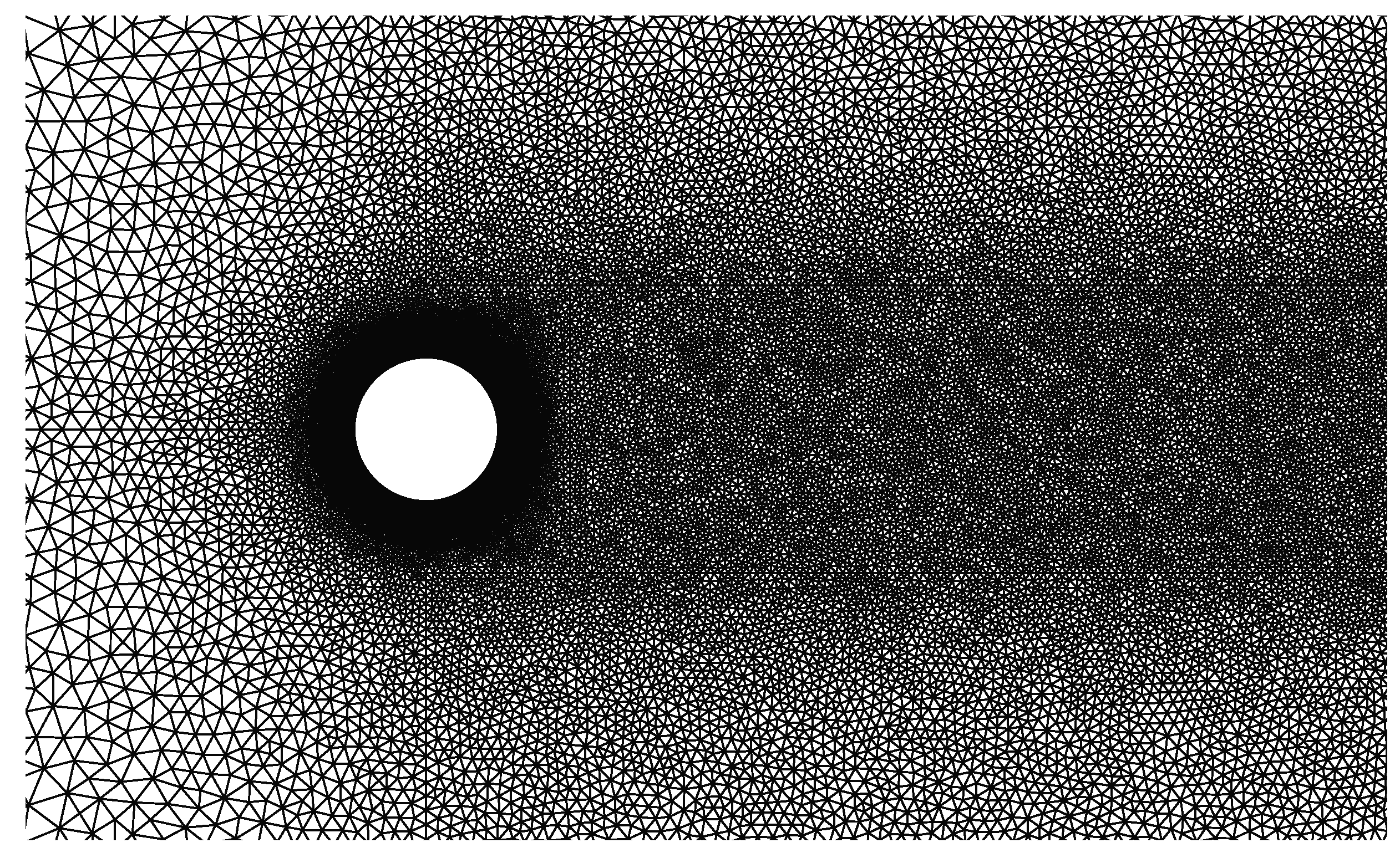
4.3.2. Computational Domain, Boundary and Initial Conditions and Mesh Generation

The domain used for the simulations is shown in Figure 7. The cylinder is located a distance L ϕ from the inlet. The total length in the streamwise direction, L > L ϕ , must be large enough so that the perturbations introduced by the cylinder become sufficiently small at the right limit of the domain for an outflow boundary condition to be used. In the simulations, the domain had a dimensionless size of L / D = 64 with L ϕ / D = 16 . Behr et al. [84] studied the influence of the distance of the lateral boundaries on the computation of two-dimensional unsteady incompressible flow past a circular cylinder. They concluded that the distance between the center of the cylinder and the lateral boundaries has a significant effect on the Strouhal number and other flow properties. In particular, they found that the minimum distance at which this influence vanishes for Re = 100 is 32 cylinder diameters. For this reason, in our simulations we chose also H / D = 64 in order to rule out any influence of the boundary conditions in the solution obtained. The Reynolds numbers chosen for the validation campaign are 100 [56,85,86] and 200 [54,77], so that the lateral boundaries are expected not to perturb the results in either case.
The boundary conditions are schematized in dimensional form in Figure 7 for non-isothermal flow past a circular cylinder at uniform temperature, to be considered in the next section. For the isothermal flow considered here, the dimensionless boundary condition for the velocity and pressure are
  • Left boundary, uniform incoming flow: u 1 = v = 0 .
  • Right boundary, outflow boundary condition: p = u / x = v = 0 .
  • Top and bottom boundaries, symmetry boundary condition: u / y = v = 0 .
  • Cylinder wall, non-slip condition: u = v = 0 .
As initial condition, the components of the velocity are set to 0 in all the points of the domain, except at the inflow boundary, where u is set to 1. The non-dimensional vertical velocity component v is set to 0 everywhere.
The strategy followed for the generation of the mesh was to use small elements in the vicinity of the cylinder and in the cylinder wake, whereas a coarser mesh was used in the rest of the domain, with the size of the elements varying gradually from the finest to the coarser regions as shown schematically in Figure 8. Several grids have been tested, from coarse to fine grids. The final grid used for the computations did not provide significantly different results than the previous coarser grid, but it was selected in order to get better estimates. In the final grid, the number of nodes was 77,011 and the number of TRIA elements was 153 318. Being D the cylinder diameter, the mesh size in the vicinity of the cylinder up to a concentric cylinder of diameter 1.1 D was 0.01 D . The mesh size in the vicinity of the previous inner cylinder up to a concentric cylinder of radius 2 D was less than 0.05 D . In a rectangular region with height 2 D , continuous to the outer concentric cylinder, the mesh size was less than 0.05 D . In the rest of the domain, the mesh size was less than 0.5 D .

4.3.3. Discussion of Results

The flow past a circular cylinder is periodic for Re = 100 . Figure 9 shows the long-term variation of the vertical velocity v in a point located at the wake of the cylinder just in the middle of the outflow boundary ( x = 64 , y = 32 ). As can be seen, after an initial transient the flow becomes periodic with a given frequency f. As can be seen in Figure 10, counter rotating eddies are shed periodically with period T = 1 / f , giving rise to the well-known Karman vortex street in the cylinder wake.
Table 2 shows the variation of the Strouhal number ( St = f D / U ) associated with the vortex shedding process corresponding to Re = 100 and different blockage ratios ( D / H ). For the smallest blockage ratio, the predicted Strouhal number perfectly matches that obtained by De Sampaio [56] (0.165), while it deviates only 0.01 % from the value obtained by Ding et al. [54] and by Rahman et al. [85] (0.164). As the Reynolds number increases the influence of the blockage ratio becomes less important, hence the mesh with blockage ratio equal to 1 / 64 has been used in the computations presented below for both Re = 100 and 200. For Re = 200 the computed Strouhal number is 0.1954, which deviates only 0.18 % from the value obtained by Qu et al. [77] (0.1958) and 0.3 % from the value obtained by Ding et al. [54] (0.196).
Table 3 compares the results obtained with DynamFluid with those of previous references. As can be seen, the Strouhal number obtained for the two Reynolds numbers considered in the study show very good agreement with the existing literature, which validates the performance of DynamFluid for the prediction of unsteady flows.

4.4. Flow Past a Heated Circular Cylinder with Forced Convection

The non-isothermal flow past a heated circular cylinder is similar to that past a non-heated cylinder with the particularity that the temperature of the cylinder, T w , is now different from the temperature of the bulk fluid, T . In the presence of buoyancy forces, the temperature variations that cause the flow to exhibit additional features due to the effects of aiding or opposing buoyancy, but for simplicity attention will be restricted here to the case where the effects of buoyancy can be neglected. As the main difference with the mixed convection problem in a vertical channel, the Prandtl number is assumed here to be Pr = 0.71 (instead of 0.72 ) in order to match the value used in previous works used here for validation.

4.4.1. Literature Review

Flow and heat transfer in forced convection past a circular cilinder has been studied by Apelt and Ledwich [87], Dennis et al. [46] and Rashid and Ahmad [88] up to Re = 40 . Bitwas et al. [58] showed that in the absence of thermal buoyancy, the separation angle and the length of the recirculation bubble increase with the Reynolds number. They also showed that the average Nusselt number increases with increasing Reynolds number and the predicted results were in accordance with well-known experimental observations. Badr [89] studied numerically the influence of the flow direction, vertically upwards (parallel flow) vs. vertically downwards (opposing flow), accounting for buoyancy effects.

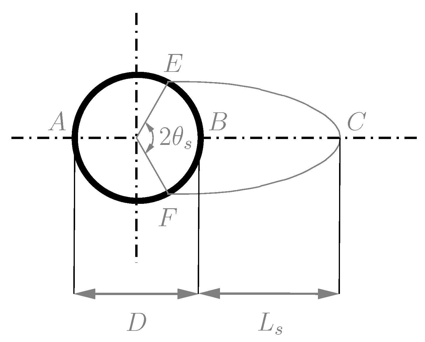
4.4.2. Computational Domain and Boundary Conditions

The computational domain used for the simulations is similar to that used in previous section, but in this case the length of the domain was reduced to L / D = 25 cylinder diameters, and the height of the domain was reduced to H / D = 20 cylinder diameters, which gives a blockage ratio of 0.05 . The center of the cylinder is located at L ϕ / D = 10 diameters from the inlet. As a result, the outflow boundary is located 15 diameters downstream the center of the cylinder. The boundary conditions imposed to the velocity and pressure fields are the same as in the previous section, with additional Dirichlet boundary conditions for the temperature ( Θ = 0 ) at the inlet and at the cylinder wall ( Θ = 1 ), zero heat flux boundary conditions at the upper and lower boundaries ( Θ / y = 0 ) as well as the outflow boundary ( Θ / x = 0 ).

4.4.3. Discussion of Results

Several simulations were carried out for increasing Reynolds numbers ranging from Re = 10 to 40 in the limit of non-buoyant flows ( Ri = Gr / Re 2 0 ). Figure 11 shows the steady-state solution reached in each simulation, including the streamlines and temperature contours obtained for the different Reynolds numbers under study. As previously reported by Williamson [90], for low Reynolds numbers ( Re < 49 ) a vertically symmetric steady wake is formed with the structure shown schematically in Figure 12. The nomenclature used to describe the flow behind the cylinder is: A is the front stagnation point, B the rear stagnation point, C the stagnation point in the cylinder wake, E and F the upper and lower separation points, L s the eddy length of the recirculation region E-C-F-B-E and ϕ s the angle with respect to the horizontal line where the fluid detaches from the cylinder. The plots in the left panels of Figure 11 show a perfect symmetry with respect to the horizontal mid-line which passes through the center of the cylinder as previously reported by Williamson [90]. The temperature gradient at the front stagnation point, the eddy length, and the separation angle all increase monotonically with the Reynolds number. For reference purposes, Table 4 shows the variation with the Reynolds number of the non-dimensional eddy length and the separation angle. Note that the eddy length is made non-dimensional with the cylinder radius ( D / 2 ) to be consistent with previous references, and that the angles are measured from the rear stagnation point. As can be seen, the results obtained with DynamFluid show excellent agreement with the values obtained by other authors [44,54,58,59] for all Reynolds numbers under study.
The local heat lost from the cylinder by heat conduction to the fluid is given by the local Nusselt number
Nu = Θ n ,
where n denotes the outward normal to the cylinder surface. The local value of Nu along the cylinder surface was computed and compared with previous results taken from the literature [46,58,89], as can be seen in Figure 13. The Nusselt number computed with DynamFluid shows good agreement with the results by Biswas et al. [58] for all Reynolds number under study, showing also good agreement in the rear stagnation point with other authors [46,89]. However, it deviates slightly in the front stagnation point from the value computed by Bard [89] and Dennis et al. [46]. The results shown in Figure 13 indicate that Badr [89] overstimated the value of the Nusselt number in the range Re = 20–40, while Dennis et al. [46] overestimated the value of the Nusselt number in the range Re = 10–40. Note that the works by Dennis et al. [46] and Bard [89] were published in 1968 and 1984, when the precision of numerical computations was still far from that of today. These results indicate that DynamFluid is able to reproduce with good agreement results of forced convection heat transfer problems, particularly those published more recently, exhibiting only local small variations that can be attributed to the imprecision of the numerical results reported decades ago.

5. Conclusions

A new CFD software tool (DynamFluid) based on the finite element method and the characteristic-based-split algorithm has been presented and validated against four benchmark constant-density and Boussinesq-type non-isothermal two-dimensional flows, showing excellent agreement with previous results taken from the literature. The test cases have comprised both stationary problems, such as the lid-driven cavity flow, mixed convection in a vertical channel, or flow past a heated circular cylinder at low Reynolds numbers, as well as unsteady problems, such as isothermal flow past a circular cylinder at moderate Reynolds numbers, covering a wide range of Reynolds, Grashof and Richardson numbers. The results provide the prospect users high confidence for the application of this software to other 2D fluid dynamic problems of interest, particularly those involving isothermal and non-isothermal incompressible flows under the Boussinesq approximation. In the near future, DynamFluid is expected to cover a broader scope of flow regimes, including fully compressible three-dimensional flows, non-constant density flows, and general non-isothermal flows.

Author Contributions

Conceptualization, H.R. and M.V.; data curation, H.R.; formal analysis, H.R., J.C. and M.V.; funding acquisition, M.V.; investigation, H.R. and M.V.; methodology, H.R. and M.V.; project administration, H.R., J.C. and M.V.; resources, H.R., P.A.G.-S. and M.V.; software, H.R. and J.C.; supervision, J.C. and M.V.; validation, H.R., P.A.G.-S. and M.V.; visualization, H.R., P.A.G.-S. and M.V.; writing–original draft, H.R. and M.V.; writing–review & editing, J.C., P.A.G.-S. and M.V.

Funding

This research was funded by FEDER/Ministerio de Ciencia, Innovación y Universidades grant numbers ENE2015-68703-C2-1-R and RTC-2017-5955-3.

Conflicts of Interest

The authors declare no conflict of interest.

Nomenclature

aSpeed of sound
BBlockage ratio ( D / H )
c p Specific heat at constant pressure
c v Specific heat at constant volume
DCylinder diameter
eInternal energy per unit mass, e = c v T
e T Total energy per unit mass, e T = e + u i u i / 2
E ¯ Energy tensor containing the values of ρ e T in every node of the mesh
E r i j Difference in the estimating function between mesh #i and mesh #j
fFrequency
gAcceleration of gravity
GrGrashof number
helement size
HCharacteristic height of the problem
I i j Identity tensor
kThermal conductivity
LCharacteristic length of the problem
L ϕ Distance from the inlet to the center of the cylinder
L s Eddy length
noutward normal coordinate
N Shape functions
NuLocal Nusselt number
pPressure
p ¯ Pressure tensor containing the values of p in every node of the mesh
PrPrandtl number, ν / α
ReReynolds number
RiRichardson number, Gr/Re 2
StStrouhal number
tTime
t ˜ i i-th component of the prescribed stress
TTemperature
T ˜ Prescribed Temperature
T ¯ Temperature tensor containing the values of T in every node of the mesh
T i ˜ i-th component of the prescribed temperature gradient
u i i-th component of the velocity vector, ( u , v , w ) T
u ¯ i Velocity tensor containing the i-th component of the velocity vector in every node of the mesh
u ˜ i i-th component of the prescribed velocity
x i i-th Cartesian coordinate, ( x , y , z ) T
Greek letters
α Thermal diffusivity, k / ( ρ c p )
β Thermal expansion coefficient, ρ 1 ( ρ / T ) p
μ Dynamic viscosity
ϕ Variable to approximate using the finite element method
ϕ s Angle of detachment
ρ Density
ν Kinematic viscosity, μ / ρ
τ i j deviatoric viscous stress tensor
θ 1 velocity relaxation factor
θ 2 pressure relaxation factor
Θ c the wall temperature difference ratio, ( T c T ) / ( T h T )
T h unstructured triangulation composed by non-overlapping elements
Subscripts
cCold boundary
hHot boundary
wWall
Reference value

References

  1. Batchelor, C.K. An Introduction to Fluid Dynamics; Cambridge University Press: Cambridge, UK, 2000; ISBN 0-521-66396-2. [Google Scholar]
  2. Van Dyke, M. An Album of Fluid Motion; The Parabolic Press: Stanford, CA, USA, 1982; ISBN 978-0915760022. [Google Scholar]
  3. Barenblatt, G.I. Dimensional Analysis; CRC Press: Amsterdam, The Netherlands, 1987; ISBN 3-7186-0438-8. [Google Scholar]
  4. Bridgman, P.W. Dimensional Analysis; Yale University Press: New Haven, CT, USA, 1922. [Google Scholar]
  5. Anderson, J.D.; Wendt, J. Computational Fluid Ddynamics; McGraw-Hill: New York, NY, USA, 1995; Volume 206. [Google Scholar]
  6. Ferziger, J.H.; Peric, M. Computational Methods for Fluid Dynamics, 3rd ed.; Springer Science Business Media: New York, NY, USA, 2012; ISBN 978-540-42074-3. [Google Scholar]
  7. Fletcher, C. Computational Techniques for Fluid Dynamics 1. Fundamental and General Techniques; Springer Science Business Media: New York, NY, USA, 1998; ISBN 978-3-642-97037-5. [Google Scholar]
  8. Fletcher, C.A. Computational Techniques for Fluid Dynamics 2: Specific Techniques for Different Flow Categories; Springer Science Business Media: New York, NY, USA, 2012; ISBN 978-3-642-97073-3. [Google Scholar]
  9. Pironneau, O. Finite Element Methods for Fluids; John Wiley & Sons: New York, NY, USA, 1989; ISBN 0-471-92255-2. [Google Scholar]
  10. Versteeg, H.K.; Malalasekera, W. An Introduction to Computational Fluid Dynamics: the Finite Volume Method; Pearson Education: Harlow, UK, 2007; ISBN 978-0-13-127498-3. [Google Scholar]
  11. ANSYS Fluent: 2019 ANSYS, Inc. Available online: https://www.ansys.com/products/fluids/ansys-fluent (accessed on 9 October 2019).
  12. Star-CCM+: 2019 Siemens Product Lifecycle Management Software Inc., All Rights Reserved. Available online: https://mdx.plm.automation.siemens.com/star-ccm-plus (accessed on 9 October 2019).
  13. COMSOL Multiphysics® v.5.4. Available online: https://www.comsol.com (accessed on 9 October 2019).
  14. Altair AcuSolve™ ©: 2019 Altair Engineering, Inc. Available online: https://altairhyperworks.com/product/AcuSolve (accessed on 9 October 2019).
  15. Weller, H.G.; Tabor, G.; Jasak, H.; Fureby, C. A tensorial approach to computational continuum mechanics using object-oriented techniques. Comput. Phys. 1998, 12, 620–631. [Google Scholar] [CrossRef]
  16. Jasak, H.; Jemcov, A.; Tukovic, Z. OpenFOAM: A C++ library for complex physics simulations. In Proceedings of the International Workshop on Coupled Methods in Numerical Dynamics, IUC, Dubrovnik, Croatia, 19–21 September 2007. [Google Scholar]
  17. OpenFOAM: OpenCFD Ltd (ESI Group). Available online: https://www.openfoam.com (accessed on 9 October 2019).
  18. Hecht, F. New development in FreeFem++. J. Numer. Math. 2012, 20, 251–266. [Google Scholar] [CrossRef]
  19. Alnaes, M.S.; Blechta, J.; Hake, J.; Johansson, A.; Kehlet, B.; Logg, A.; Richardson, C.; Ring, J.; Rognes, M.E.; Wells, G.N. The FEniCS Project Version 1.5. Arch. Numer. Soft. 2015, 3, 9–23. [Google Scholar] [CrossRef]
  20. Ahrens, J.; Geveci, B.; Law, C. ParaView: An End-User Tool for Large-Data Visualization. In The Visualization Handbook; Hansen, C.D., Johnson, C.R., Eds.; Elsevier Butterworth-Heinemann: Amsterdam, The Netherlands, 2005; pp. 717–731. ISBN 978-0-12-387582-2. [Google Scholar]
  21. Eigen: GNU Free Documentation License 1.2. Available online: http://eigen.tuxfamily.org (accessed on 9 October 2019).
  22. AbdelMigid, T.A.; Saqr, K.M.; Kotb, M.A.; Aboelfarag, A.A. Revisiting the lid-driven cavity flow problem: Review and new steady state benchmarking results using GPU accelerated code. Alex. Eng. J. 2017, 56, 123–135. [Google Scholar] [CrossRef] [Green Version]
  23. Erturk, E.; Corke, T.C.; Gökçöl, C. Numerical solutions of 2D steady incompressible driven cavity flow at high Reynolds numbers. Int. J. Numer. Methods Fluids 2005, 48, 747–774. [Google Scholar] [CrossRef]
  24. Erturk, E. Discussions on driven cavity flow. Int. J. Numer. Methods Fluids 2009, 60, 275–294. [Google Scholar] [CrossRef]
  25. Yapici, K.; Uludag, Y. Finite volume simulation of 2-D steady square lid-driven cavity flow at high reynolds numbers. Braz. J. Chem. Eng. 2013, 30, 923–937. [Google Scholar] [CrossRef]
  26. Ghia, U.; Ghia, K.N.; Shin, C.T. High-Re Solutions for incompressible flow using the Navier-Stokes equations and a multigrid method. J. Comput. Phys. 1982, 48, 387–411. [Google Scholar] [CrossRef]
  27. Marchi, C.H.; Suero, R.; Araki, L.K. The lid-driven square cavity flow: Numerical solution with a 1024 x 1024 grid. J. Braz. Soc. Mech. Sci. 2009, 31, 186–198. [Google Scholar] [CrossRef]
  28. Zhen-Hua, C.; Bao-Chang, S.; Lin, Z. Simulating high Reynolds number flow in two-dimensional lid-driven cavity by multi-relaxation-time lattice Boltzmann method. Chin. Phys. 2006, 15, 1855. [Google Scholar] [CrossRef]
  29. Erturk, E.; Dursun, B. Numerical solutions of 2-D steady incompressible flow in a driven skewed cavity. ZAMM Z. Angew. Math. Mech. 2007, 87, 377–392. [Google Scholar] [CrossRef] [Green Version]
  30. Aung, W.; Worku, G. Developing flow and flow reversal in a vertical channel with asymmetric wall temperatures. J. Heat Transf. 1986, 108, 299–304. [Google Scholar] [CrossRef]
  31. Aung, W.; Worku, G. Mixed convection in ducts with asymmetric wall heat fluxes. J. Heat Transf. 1987, 109, 947–951. [Google Scholar] [CrossRef]
  32. Aung, W.; Worku, G. Theory of fully developed, combined convection including flow reversal. J. Heat Transf. 1986, 108, 485–488. [Google Scholar] [CrossRef]
  33. Barletta, A. Analysis of flow reversal for laminar mixed convection in a vertical rectangular duct with one or more isothermal walls. Int. J. Heat Mass Transf. 2001, 44, 3481–3497. [Google Scholar] [CrossRef]
  34. Barletta, A.; Magyari, E.; Keller, B. Dual mixed convection flows in a vertical channel. Int. J. Heat Mass Transf. 2005, 48, 4835–4845. [Google Scholar] [CrossRef]
  35. Boulama, K.; Galanis, N. Analytical solution for fully developed mixed convection between parallel vertical plates with heat and mass transfer. J. Heat Transf. 2004, 126, 381–388. [Google Scholar] [CrossRef]
  36. Cheng, C.H.; Kou, H.S.; Huang, W.H. Flow reversal and heat transfer of fully developed mixed convection in vertical channels. J. Thermophys. Heat Transf. 1990, 4, 375–383. [Google Scholar] [CrossRef]
  37. El-Din, M.S. Effect of thermal and mass buoyancy forces on the development of laminar mixed convection between vertical parallel plates with uniform wall heat and mass fluxes. Int. J. Therm. Sci. 2003, 42, 447–453. [Google Scholar] [CrossRef]
  38. Gau, C.; Yih, K.A.; Aung, W. Reversed flow structure and heat transfer measurements for buoyancy-assisted convection in a heated vertical duct. J. Heat Transf. 1992, 114, 928–935. [Google Scholar] [CrossRef]
  39. Hamadah, T.T.; Wirtz, R.A. Analysis of laminar fully developed mixed convection in a vertical channel with opposing buoyancy. J. Heat Transf. 1991, 113, 507–510. [Google Scholar] [CrossRef]
  40. Ingham, D.B.; Keen, D.J.; Heggs, P.J. Flows in vertical channels with asymmetric wall temperatures and including situations where reverse flows occur. J. Heat Transf. 1988, 110, 910–917. [Google Scholar] [CrossRef]
  41. Ingham, D.B.; Keen, D.J.; Heggs, P.J. Two dimensional combined convection in vertical parallel plate ducts, including situations of flow reversal. Int. J. Numer. Methods Eng. 1988, 26, 1645–1664. [Google Scholar] [CrossRef]
  42. Jeng, Y.N.; Chen, J.L.; Aung, W. On the Reynolds-number independence of mixed convection in a vertical channel subjected to asymmetric wall temperatures with and without flow reversal. Int. J. Heat Fluid Flow 1992, 13, 329–339. [Google Scholar] [CrossRef]
  43. Kim, S.H.; Anand, N.K.; Aung, W. Effect of wall conduction on free convection between asymmetrically heated vertical plates: Uniform wall heat flux. Int. J. Heat Mass Transf. 1990, 33, 1013–1023. [Google Scholar] [CrossRef]
  44. Dennis, S.C.R.; Chang, G.-Z. Numerical solutions for steady flow past a circular cylinder at Reynolds number up to 100. J. Fluid Mech. 1970, 42, 471–489. [Google Scholar] [CrossRef]
  45. Dennis, S.C.R.; Hudson, J.D. An h4 accurate vorticity-velocity formulation for calculating flow past circular cylinder. Int J. Numer. Methods Fluids 1995, 21, 489–497. [Google Scholar] [CrossRef]
  46. Dennis, S.C.R.; Hudson, J.D.; Smith, N. Steady laminar forced convection from a circular cylinder at low Reynolds numbers. Phys. Fluids 1968, 11, 933–940. [Google Scholar] [CrossRef]
  47. Grove, A.S.; Shair, F.H.; Petersen, E.E. An experimental investigation of the steady separated flow past a circular cylinder. J. Fluid Mech. 1964, 19, 60–80. [Google Scholar] [CrossRef]
  48. Norberg, C. Pressure forces on a circular cylinder in cross flow. In Bluff-Body Wakes, Dynamics and Instabilities; Eckelmann, H., Graham, J.M.R., Huerre, P., Monkewitz, P.A., Eds.; Springer: Berlin/Heidelberg, Germany, 1993; pp. 275–278. ISBN 978-3-662-00414-2. [Google Scholar]
  49. Norberg, C. An experimental investigation of the flow around a circular cylinder: Influence of aspect ratio. J. Fluid Mech. 1994, 258, 287–316. [Google Scholar] [CrossRef]
  50. Norberg, C. Flow around a circular cylinder: Aspects of fluctuating lift. J. Fluid Struct. 2001, 15, 459–469. [Google Scholar] [CrossRef]
  51. Norberg, C. Fluctuating lift on a circular cylinder: Review and new measurements. J. Fluid Struct. 2003, 17, 57–96. [Google Scholar] [CrossRef]
  52. Triton, D.J. Experiments on the flow past a circular cylinder at low Reynolds number. J. Fluid Mech. 1959, 6, 547–567. [Google Scholar] [CrossRef]
  53. Chakraborty, J.; Verma, N.; Chhabra, R.P. Wall effects in the flow past a circular cylinder in a plane channel: A numerical study. Chem. Eng. Process. 2004, 43, 1529–1537. [Google Scholar] [CrossRef]
  54. Ding, H.; Shu, C.; Yeo, K.S.; Xu, D. Simulation of incompressible viscous flows past a circular cylinder by hybrid FD scheme and meshless least square-based finite difference scheme. Comput. Methods Appl. Mech. 2004, 193, 727–744. [Google Scholar] [CrossRef]
  55. Park, J.; Kwon, K.; Choi, H. Numerical solutions of flow past a circular cylinder at Reynolds numbers up to 160. KSME Int. J. 1998, 12, 1200–1205. [Google Scholar] [CrossRef]
  56. De Sampaio, P.A.B.; Lyra, P.R.M.; Morgan, K.; Weatherill, N.P. Petrov-Galerkin solutions of the incompressible Navier-Stokes equations in primitive variables with adaptative remeshing. Comput. Methods Appl. Mech. 1993, 106, 143–178. [Google Scholar] [CrossRef]
  57. Subhankar, S.; Sanjay, M.; Gautam, B. Numerical Simulation of Steady Flow Past a Circular Cylinder. In Proceedings of the 37th National and 4th International Conference on Fluid Mechanics and Fluid Power, IIT Madras, Chennai, India, 16–18 December 2010. [Google Scholar]
  58. Bitwas, G.; Sarkar, S. Effect of thermal buoyancy on vortex shedding past a circular cylinder in cross-flow at low Reynolds numbers. Int J. Heat Mass Transf. 2009, 52, 1897–1912. [Google Scholar] [CrossRef]
  59. Takami, H.; Keller, H.B. Steady two-dimensional viscous flow of an incompressible fluid past a circular cylinder. Phys. Fluids 1969, 12, II-51–II-56. [Google Scholar] [CrossRef]
  60. Zienkiewicz, O.C.; Morgan, K.; Satya Sai, B.V.K.; Codina, R.; Vazquez, M. A general algorithm for compressible and incompressible flow—Part II. Tests on the explicit form. Int. J. Numer. Methods Fluids 1995, 20, 887–913. [Google Scholar] [CrossRef]
  61. Zienkiewicz, O.C.; Codina, R. A general algorithm for compressible and incompresible flow - Part I. The split, characteristic based scheme. Int. J. Numer. Methods Fluids 1996, 20, 869–885. [Google Scholar] [CrossRef]
  62. Zienkiewicz, O.C.; Nithiarasu, P.; Codina, R.; Vazquez, M.; Ortiz, P. The characteristic-based-split procedure: An efficient and accurate algorithm for fluid problems. Int. J. Numer. Methods Fluids 1999, 31, 359–392. [Google Scholar] [CrossRef]
  63. Zienkiewicz, O.C.; Taylor, R.L. The Finite Element Method. Volume 3: Fluid Dynamics, 6th ed.; Elsevier Butterworth-Heinemann: Amsterdam, The Netherlands, 2005; ISBN 0-7506-6322-7. [Google Scholar]
  64. Nithiarasu, P.; Codina, R.; Zienkiewicz, O.C. The Characteristic-Based Split (CBS) scheme—A unified approach to fluid dynamics. Int. J. Numer. Methods Eng. 2006, 66, 1514–1546. [Google Scholar] [CrossRef]
  65. Chorin, A.J. A numerical method for solving incompressible viscous flow problems. J. Comput. Phys. 1967, 2, 12–26. [Google Scholar] [CrossRef]
  66. Codina, R.; Vazquez, M.; Zienkiewicz, O.C. A general algorithm for compressible and incompressible flows. Part III: The semi-implicit form. Int. J. Numer. Methods Fluids 1998, 27, 13–32. [Google Scholar] [CrossRef]
  67. Editorial Board. Georgii Ivanovich Petrov (on his 100th birthday). Fluid Dyn. 2012, 47, 289–291. [Google Scholar] [CrossRef]
  68. Ern, A.; Guermond, J.L. Theory and Practice of Finite Elements; Springer: New York, NY, USA, 2004; ISBN 9780387205748. [Google Scholar]
  69. Mikhlin, S.G. Variational Methods in Mathematical Physics; Pergamon Press: New York, NY, USA, 1964. [Google Scholar]
  70. Carpio, J.; Prieto, J.L.; Vera, M. A local anisotropic adaptive algorithm for the solution of low-Mach transient combustion problems. J. Comput. Phys. 2016, 306, 19–42. [Google Scholar] [CrossRef]
  71. Lewis, R.W.; Nithiarasu, P.; Seetharamu, K.N. Fundamentals of the Finite Element Method for Heat and Fluid Flow; Wiley: West Sussex, UK, 2004; ISBN 978-0-470-02081-4. [Google Scholar]
  72. Roache, P.J. Quantification of uncertainty in computational fluid dynamics. Annu. Rev. Fluid Mech. 1997, 29, 123–160. [Google Scholar] [CrossRef]
  73. Desrayaud, G.; Lauriat, G. Flow reversal of laminar mixed convection in the entry region of symmetrically heated, vertical plate channels. Int. J. Therm. Sci. 2009, 48, 2036–2045. [Google Scholar] [CrossRef]
  74. Nithiarasu, P. An efficient artificial compressibility (AC) scheme based on the characteristic based split (CBS) method for incompressible flows. Int. J. Numer. Methods Eng. 2003, 5, 1815–1845. [Google Scholar] [CrossRef]
  75. Massarotti, N.; Arpino, F.; Lewis, R.W.; Nithiarasu, P. Explicit and semi-implicit CBS procedures for incompressible viscous flows. Int. J. Numer. Methods Eng. 2006, 66, 1618–1640. [Google Scholar] [CrossRef]
  76. Selvam, R.P. Finite element modelling of flow around a circular cylinder using LES. J. Wind Eng. Ind. Aerod. 1997, 67, 129–139. [Google Scholar] [CrossRef]
  77. Qu, L.; Norgerg, C.; Davidson, L.; Peng, S.; Wang, F. Quantitive numerical analysis of flow past a circular cylinder at Reynolds number between 50 and 200. J. Fluid Struct. 2013, 39, 347–370. [Google Scholar] [CrossRef]
  78. Sahin, M.; Owens, R.G. A numerical investigation of wall effects up to high blockage ratios on two-dimensional flow past a confined circular cylinder. Phys. Fluids 2004, 16, 1305–1320. [Google Scholar] [CrossRef]
  79. Posdziech, O.; Grundmann, R. A systematic approach to the numerical calculation of fundamental quantities of the two-dimensional flow over a circular cylinder. J. Fluid Struct. 2007, 23, 479–499. [Google Scholar] [CrossRef]
  80. Mittal, S.; Raghuvanshi, A. Control of vortex shedding behind circular cylinder for flows at low Reynolds numbers. Int. J. Numer. Methods Fluids 2001, 35, 421–447. [Google Scholar] [CrossRef]
  81. Mittal, S.; Kumar, V. Finite element study of vortex-induced cross-flow and in-line oscillations of a circular cylinder at low Reynolds numbers. Int. J. Numer. Methods Fluids 1999, 31, 1087–1120. [Google Scholar] [CrossRef]
  82. Kieft, R.; Rindt, C.C.M.; van Steenhoven, A.A. Near-weak effects of a heat input on the vortex-shedding mechanism. Int. J. Heat Fluid Flow 2007, 28, 938–947. [Google Scholar] [CrossRef]
  83. Jordan, S.A.; Ragab, S.A. A large-eddy simulation of the near wake of a circular cylinder. J. Fluid Eng. 1998, 120, 243–252. [Google Scholar] [CrossRef]
  84. Behr, M.; Hastreiter, D.; Mittal, S.; Tezduyar, T.E. Incompressible flow past a circular cylinder: Dependence of the computed flow field on the location of the lateral boundaries. Comput. Methods Appl. Mech. 1995, 123, 309–316. [Google Scholar] [CrossRef]
  85. Rahman, M.; Karim, M.; Alim, A. Numerical investigation of unsteady flow past a circular cylinder using 2-D Finite Volume Method. JNAME 2007, 4, 27–42. [Google Scholar] [CrossRef]
  86. Rajani, B.N.; Kandasamy, A.; Majumdar, S. Numerical simulation of laminar flow past a circular cylinder. Appl. Math. Model. 2009, 33, 1228–1247. [Google Scholar] [CrossRef]
  87. Apelt, C.J.; Ledwich, M.A. Heat transfer in transient and unsteady flows past a circular cylinder in the range 1 < R < 40. J. Fluid Mech. 1979, 95, 761–777. [Google Scholar] [CrossRef]
  88. Rashid, A.; Ahmad, P.H. Steady-State Numerical Solution of the Navier-Stokes and Energy Equations around a Horizontal Cylinder at Moderate Reynolds Numbers from 100 to 500. Heat Transf. Eng. 1996, 17, 31–81. [Google Scholar] [CrossRef]
  89. Badr, H.M. Laminar combined convection from a horizontal cylinder—Parallel and contra flow regimes. Int. J. Heat Mass Transf. 1984, 27, 15–27. [Google Scholar] [CrossRef]
  90. Williamson, C.H.K. Vortex dynamics in the cylinder wake. Annu. Rev. Fluid Mech. 1996, 28, 477–539. [Google Scholar] [CrossRef]
Figure 1. Schematic representation of the lid-driven cavity flow showing the coordinate system, dimensional parameters, and boundary conditions.
Processes 07 00777 g001
Figure 2. Convergence analysis for the horizontal velocity along the vertical mid line corresponding to Re = 1000 (left) and triangular elements (TRIA) 20 × 20 element mesh used in the computations with DynamFluid (right). The 50 × 50 and 100 × 100 meshes are finer meshes with the same topology.
Processes 07 00777 g002
Figure 3. Two-dimensional finite elements adjacent to node k used to compute the equivalent element size h k = min ( 2 A j / l j ) .
Processes 07 00777 g003
Figure 4. Horizontal velocity along the vertical mid line (left) and vertical velocity along the horizontal mid line (right) as predicted by DynamFluid (solid lines) and reported by Erturk [24] (⋄) and Ghia et al. [26] (+) for Re = { 400 , 1000 , 25 , 000 , 5000 , 10 , 000 } .
Processes 07 00777 g004
Figure 5. Schematic representation of the non-isothermal flow in a vertical channel with asymmetric wall temperatures showing the coordinate system, dimensional parameters, and boundary conditions.
Processes 07 00777 g005
Figure 6. Comparison between the fully developed velocity (left) and temperature (right) profiles as predicted by DynamFluid (solid lines) and by the fully developed theory of Aung and Worku [32] (symbols) corresponding to Re = 100 , Gr = 25,000, and Θ c = { 0 , 0 . 5 } .
Processes 07 00777 g006
Figure 7. Schematic representation of the flow past a circular cylinder showing the coordinate system, dimensional parameters, and boundary conditions. The size of the computational domain is determined by the parameters L, L ϕ and H.
Processes 07 00777 g007
Figure 8. Close-up view of the mesh in the vicinity of the cylinder and in the wake.
Processes 07 00777 g008
Figure 9. Vertical velocity v in the mid plane far downstream the cylinder for Re = 100 .
Processes 07 00777 g009
Figure 10. Vorticity field of the flow past a circular cylinder for Re = 100 at four successive instants during the vortex shedding cycle.
Processes 07 00777 g010
Figure 11. Streamlines and temperature contours of the steady state solution for several Reynolds numbers and Ri = 0: (a) Re = 10, (b) Re = 15, (c) Re = 20, (d) Re = 25, and (e) Re = 40. The color map in the left plots represents the modulus of the velocity vector.
Processes 07 00777 g011
Figure 12. Schematic description of the recirculation region showing the dimensionless eddy length ( L s ) and the separation angle ( θ s ).
Processes 07 00777 g012
Figure 13. Variationof the local Nusselt number on the surface of the cylinder at different Reynolds number as predicted by DynamFluid (solid lines) and by previous authors.
Processes 07 00777 g013
Table 1. Mean and max error for the horizontal velocity.
Grid Comparison Er L 1 Er L r ij
50 × 50 vs. 20 × 20 0.00176 0.00748 2.0
100 × 100 vs. 50 × 50 0.0138 0.0969 2.5
Table 2. Strouhal number as a function of the blockage ratio for Re = 100 .
D / H St
1 / 16 0.1792
1 / 32 0.1703
1 / 64 0.1650
Table 3. Comparison between the Strouhal number for Re = { 100 , 200 } as predicted by DynamFluid and reported by previous authors.
Re [56] [77] [86] [85] [54]Present Work
100 0.165 0.1649 0.1569 0.164 0.164 0.165
200 0.1958 0.1957 0.196 0.1954
Table 4. Comparison between the eddy length ( L s ) and the separation angle ( θ s ) for several Reynolds numbers as predicted by DynamFluid and reported by previous authors.
Variable Re [44] [59] [58] [54] [55]DynamFluid
10 0.504 0.498 0.52 0.504 0.51 0.512
15 1.162 1.189 1.227
2 L s / D 20 1.88 1.844 1.865 1.86 1.87 1.866
25 2.517 2.548
40 4.69 4.65 4.424 4.4 4.59 4.480
Variable Re [44] [59] [58] [54] [55]DynamFluid
10 29.6 29.3 29.12 30.0 28.57
15 38.6 38.57 38.57
θ s ( )20 43.7 43.65 43.64 44.1 43.58
25 46.89 47.14
40 53.8 53.55 53.1 53.5 51.43

