Article

A General Model for Estimating Emissions from Integrated Power Generation and Energy Storage. Case Study: Integration of Solar Photovoltaic Power and Wind Power with Batteries

1
MIT Energy Initiative, Massachusetts Institute of Technology, 77 Massachusetts Avenue, Cambridge, MA 02139, USA
2
Department of Chemical Engineering, Massachusetts Institute of Technology, 77 Massachusetts Avenue, Cambridge, MA 02139, USA
*
Author to whom correspondence should be addressed.
Processes 2018, 6(12), 267; https://doi.org/10.3390/pr6120267
Submission received: 17 October 2018 / Revised: 5 December 2018 / Accepted: 8 December 2018 / Published: 18 December 2018
(This article belongs to the Special Issue Modeling and Simulation of Energy Systems)

Abstract

:
The penetration of renewable power generation is increasing at an unprecedented pace. While the operating greenhouse gas (GHG) emissions of photovoltaic (PV) and wind power are negligible, their upstream emissions are not. The great challenge with the deployment of renewable power generators is their intermittent and variable nature. Current electric power systems balance these fluctuations primarily using natural gas fired power plants. Alternatively, these dynamics could be handled by the integration of energy storage technologies to store energy during renewable energy availability and discharge when needed. In this paper, we present a model for estimating emissions from integrated power generation and energy storage. The model applies to emissions of all pollutants, including greenhouse gases (GHGs), and to all storage technologies, including pumped hydroelectric and electrochemical storage. As a case study, the model is used to estimate the GHG emissions of electricity from systems that couple photovoltaic and wind generation with lithium-ion batteries (LBs) and vanadium redox flow batteries (VFBs). To facilitate the case study, we conducted a life cycle assessment (LCA) of photovoltaic (PV) power, as well as a synthesis of existing wind power LCAs. The PV LCA is also used to estimate the emissions impact of a common PV practice that has not been comprehensively analyzed by LCA—solar tracking. The case study of renewables and battery storage indicates that PV and wind power remain much less carbon intensive than fossil-based generation, even when coupled with large amounts of LBs or VFBs. Even the most carbon intensive renewable power analyzed still emits only ~25% of the GHGs of the least carbon intensive mainstream fossil power. Lastly, we find that the pathway to minimize the GHG emissions of power from a coupled system depends upon the generator. Given low-emission generation (<50 gCO2e/kWh), the minimizing pathway is the storage technology with lowest production emissions (VFBs over LBs for our case study). Given high-emission generation (>200 gCO2e/kWh), the minimizing pathway is the storage technology with highest round-trip efficiency (LBs over VFBs).

1. Introduction

1.1. Background

The electric power sector produces 40% of global greenhouse gas (GHG) emissions [1]. To limit human-caused global warming to 2 °C, the International Energy Agency (IEA) projects that power sector emissions must decline by 90% by 2050, from 13 to 1.4 gigatons of carbon dioxide per year [1]. To help achieve this decline, many governments have increased their support for low-carbon power sources. Because of this support and large cost reductions [2], photovoltaic (PV) and wind power have grown from ~1% of global electricity in 2007, to ~6% in 2017 [3], and are projected to reach 15–33% by 2040 [4,5]. The most widely deployed PV cell types are multi-crystalline silicon (mc-Si), single-crystalline silicon (sc-Si), and cadmium telluride (CdTe), with market shares of 70%, 24%, and 4%, respectively, of new PV capacity installed in 2016 [6]. The most widely deployed wind turbines are 1.6–3 MW models installed at onshore wind farms, with generation from larger offshore turbines comprising a small but growing share of the total (5% in 2017) [7,8].
While the operating GHG emissions of PV and wind power are negligible, their upstream emissions are not. To be concise, this paper refers to the total life cycle GHG emissions of AC electricity as “carbon intensity”, and the units of grams-CO2-equivalent/kilowatthour as “gCO2e/kWh”. The carbon intensity of PV power has been estimated at 76, 53, and 27 gCO2e/kWh for sc-Si, mc-Si, and CdTe PV, respectively, installed in northern Europe circa 2015, and at 33, 22, and 13 gCO2e/kWh for PV installed in the United States Southwest circa 2015 [9]. The carbon intensity of wind power has been estimated at approximately 12, 10, and 9 gCO2e/kWh, respectively, for onshore wind farms in low, medium, and high wind-speed areas, respectively, and at 14 gCO2e/kWh for offshore wind farms (which are typically located in high wind-speed areas) [10,11,12,13,14,15,16,17,18]. For context, representative GHG emissions from combined cycle natural gas (CCNG) and supercritical pulverized coal power (SCPC) are approximately 488 and 965 gCO2e/kWh, respectively [19].
The leading method for estimating carbon intensity is the life cycle assessment (LCA). As outlined by ISO standards 14040 and 14044 [ISO], LCA quantifies a product’s environmental impacts through the input–output accounting of cradle-to-grave or cradle-to-gate processes. Since 2007, over 50 studies have conducted LCA of PV power, and have found that the top drivers of PV carbon intensity are upstream electricity source, cell type, module efficiency, irradiance at installation site, and system lifetime [20,21]. Peng et al. [20] provided a detailed literature review of PV LCA and underlined gaps in the field, including the treatment of cell temperature and module orientation. IEA reports from 2008, 2011, and 2016 [22] provided methodology guidelines for PV LCA.
Important differences between this work and prior LCAs include the following: (1) This work addresses a major development in PV that prior LCAs have not addressed in depth or with explanatory equations (solar tracking); and (2) this work provides a model and equations that show how to estimate emissions from coupled generation and storage, whereas prior battery LCAs have focused on modeling emissions from battery production.

1.2. Motivation for PV LCA

One major development in PV power production, the growth of solar tracking, has not been comprehensively analyzed by LCA. In the United States from 2008 to 2014, only 19% of new utility-scale (AC capacity >5 MW) CdTe projects had tracking (16 of 86 projects); in 2015 and 2016, the number was 56% (44 of 79 projects), including locations outside the exceptionally sunny United States Southwest, such as Colorado, Tennessee, and Georgia [8]. For all cell types, tracking was used on 53% of cumulative panel capacity and 70% of new capacity at utility-scale sites in the United States in 2016 [8]. Several LCAs have analyzed the emissions impact of solar tracking, but with a limited geographic scope and with tracking set-ups that are not (and do not claim to be) representative of industry practice [23,24,25]. Bayod-Rújula [23] analyzed a two-axis tracking system in Spain. Beylot et al. [25] and Desideri et al. [24] analyzed hypothetical one-axis tracking systems with a 30° tilt in Italy. In contrast, the industry norm for PV tracking is horizontal one-axis tracking; in the United States in 2016, 97% of utility-scale tracking PV projects used horizontal one-axis tracking (255 of 263 projects) [26].
Two PV LCAs did analyze industry-representative tracking set-ups. Leccisi et al. [9] found that horizontal one-axis tracking reduced carbon intensity by 11% and 1% for mc-Si and CdTe PV, respectively, given installation in the United States Southwest. Sinha et al. [27] estimated that tracking reduced the carbon intensity of CdTe PV by 3% in the United States Southwest. However, neither study calculated tracking’s impact outside the United States Southwest. This paper aims to build on these studies by calculating tracking’s impact on PV carbon intensity over a range of locations.

1.3. Motivation for Modeling Emissions from Coupled Generation and Energy Storage

A barrier to the continued growth of both PV and wind power, and one reason that projections span a large range, is intermittency and uncertainties over how intermittency will be managed as renewables grow. As PV rises above 20% of daily generation in a region, this can lead to curtailment of existing PV, less favorable economics for future PV, and inefficient “peaker” use of other power systems, including gas-fired turbines [28,29]. “Peaker” power plants are only used to meet peak demand and are otherwise are idle. Similar dynamics apply to wind at a high penetration [30,31].
Energy storage can contribute to solving the challenges of intermittency. Storage coupled with generation has the potential to (1) flatten power supplied by intermittents to the grid, and (2) reduce peak generation and thus capacity required of non-intermittents. Partly because of this potential, the growth of non-hydro storage capacity in the United States has been accelerating, from ~1000 MWh added between 2013 and 2017, to a projected ~1000 MWh in 2018, and more in each year through 2023 [32]. Lithium-ion batteries (LBs) and vanadium redox flow batteries (VFBs) are two of the most common non-hydro storage types. LBs constitute a large majority of current and projected non-hydro storage deployment [32]. VFBs constitute a significant share of utility-scale storage installations with durations over 3 h [33]. Storage duration is the ratio of rated storage energy capacity to rated storage power capacity, and represents the time required to discharge the fully charged storage unit at its rated power output. This paper focuses on storage applications that require durations of 3 to 7 h, such as smoothing intermittent generation to better match demand.
While coupling storage with generation can mitigate intermittency, the impact on the GHG emissions of electricity supply is less well understood. Spanos et al. [34] conducted cradle-to-gate LCAs of lead–acid, nickel–zinc, and manganese dioxide–zince batteries, and thus estimated their GHG emissions per battery mass produced. The authors did not analyze the operating life or coupling of the batteries with generation. Rydh and Sandén [35] evaluated the energy required to produce eight common battery types, including LBs, VFBs, lead–acid batteries (LABs), and sodium sulfur batteries (SSBs), and found that, on a mass basis, LABs require significantly more energy to be produced than LBs or VRBs. Denholm et al. [36] analyzed the coupling of generation with VRBs, pumped hydro storage (PHS), and compressed air energy storage (CAES). The authors found that electricity from nuclear or renewables coupled with PHS had a lower carbon intensity than electricity from nuclear or renewables coupled with VRBs or CAES. On the other hand, with fossil generation, systems employing CAES had significantly lower GHG emissions than those with VRBs or PHS. Denholm et al. and Mitavachan et al. [37] both emphasized that the carbon intensity of electricity from a coupled system depended on both generation type and energy storage type.
These prior battery LCAs have comprehensively modeled production of the most common battery types for power plant applications. This paper complements these prior works by presenting an easy to implement model to estimate emissions from a combined generation and storage system. The model is general and applies to emissions of all pollutants, not just GHGs, and to all storage methods, not only electrochemical. As a case study, we used the model to estimate the impact of adding LBs and VFBs to typical mainstream PV, wind, gas, and coal-based generation.

2. Methodology

2.1. Model of Combined Generation and Storage

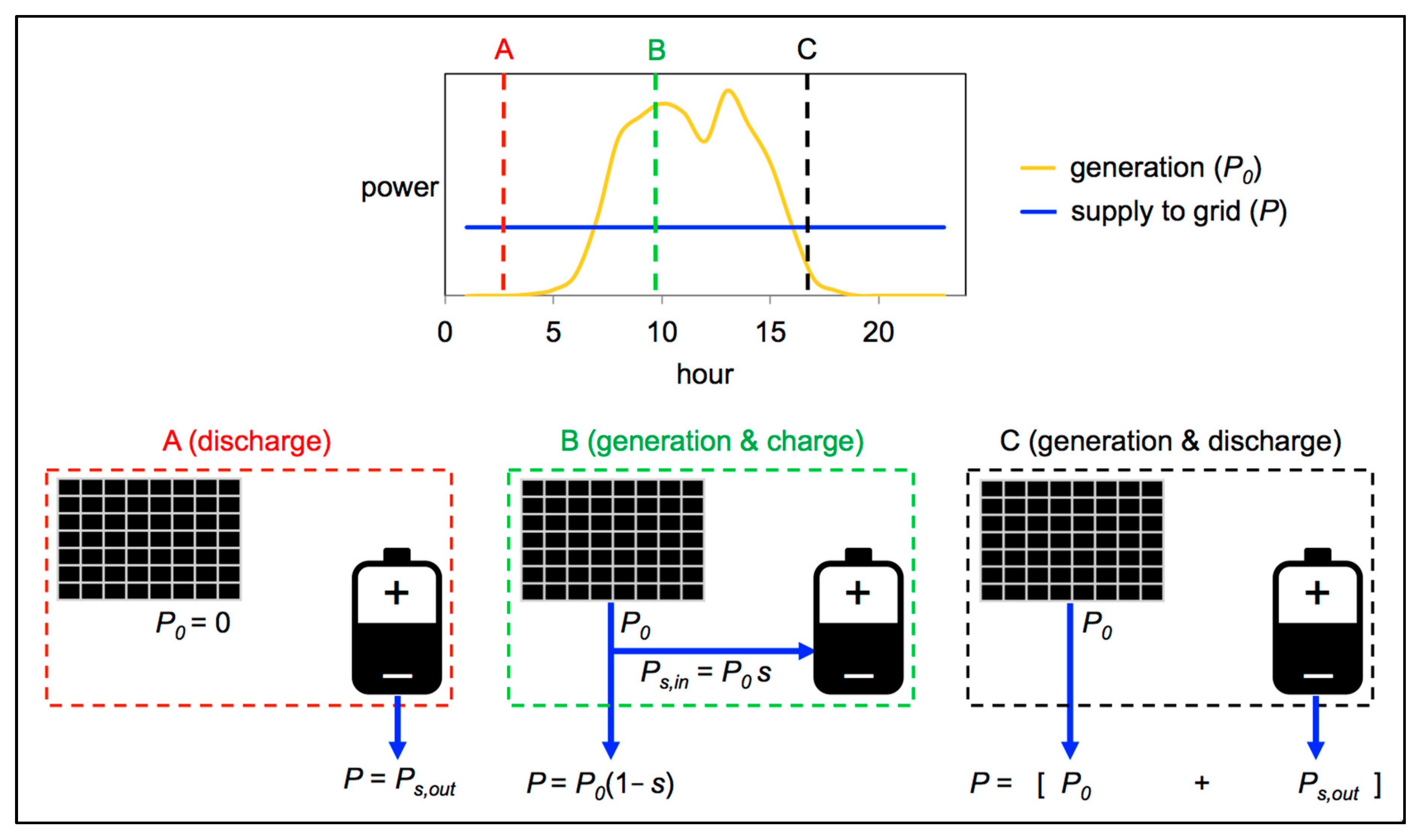
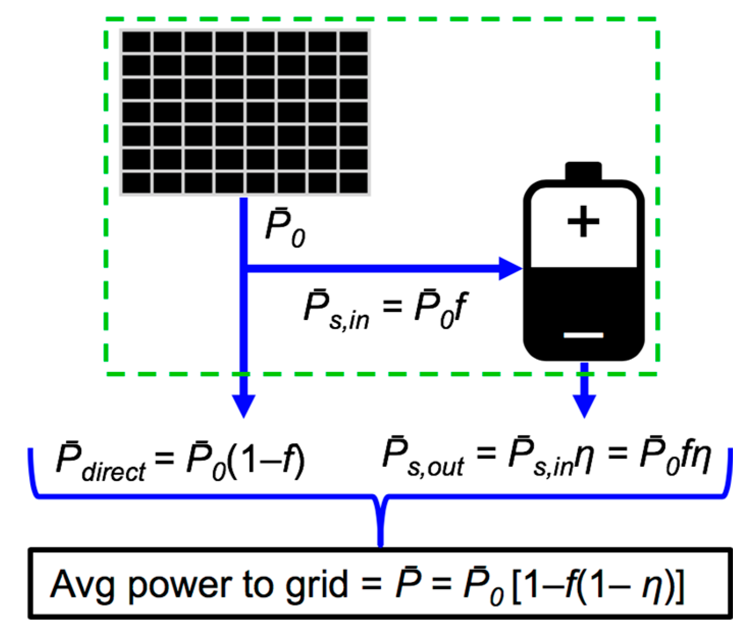
2.1.1. Model of Electricity Supply to Grid

Figure 1 shows an example of a generation curve (yellow) and a supply curve (blue). The generation curve shows how much electric power the generator is producing, while the supply curve shows how much power is supplied to the grid. When supply exceeds generation, the difference comes from storage, and when generation exceeds supply, the difference goes to storage. In Figure 1, typical variable PV generation is converted to constant supply. This is a simple example to illustrate the model. Infinite shapes are possible for the two curves, as long as the area under the supply curve does not exceed the area under the generation curve. The area under the supply curve will always be less than the area under the generation curve, because of round-trip efficiency losses in storage.
Averaging the power flows in Figure 1 produces Figure 2, which shows how the average power to grid can be calculated, as follows:
P ¯ = P ¯ 0 [ 1 f ( 1 η ) ]
where η is the round-trip efficiency of the storage, and f is the fraction of the energy generation sent to storage (vs. directly to grid). f is the generation-weighted average of s (<sP0>/<P0>), not the time-average (<s>). The lifetime electricity to grid can then be calculated as follows:
E = t P ¯ = t P ¯ 0 [ 1 f ( 1 η ) ] = E 0 [ 1 f ( 1 η ) ]
f depends on the generation and supply curves. Figure 3 illustrates this dependence, as well as how f changes with the degree of peak-smoothing.
Figure 3 shows the minimum storage energy capacity and power capacity needed to convert the given generation to the desired supply. This paper does not attempt to prescribe the optimum amounts of storage energy capacity, storage power capacity, or generation curtailment for a given desired f. For example, developers of a combined PV and storage plant that aims for constant supply must decide whether to install enough storage energy capacity to maintain a supply to the grid for three or four or more consecutive cloudy days. These decisions involve risk-analyses and design choices that are beyond the scope of this paper. This paper provides tools to estimate how those different design choices impact emissions.

2.1.2. Model Equations and Parameters

Without storage, the emissions intensity I (g/kWh) of the power generated and delivered to the grid can be calculated as follows:
I 0 = e g / E 0
where e g is the life emissions of the generator (g), and E 0 is the life electricity generated (kWh). The subscripts 0 in I 0 and E 0 indicate the no-storage base case. In this paper, the generator is assumed to operate nearly identically in the no-storage and storage-added cases, with the only difference being that, in the latter case, some of the generation is sent through storage on its way to the grid. In reality, the addition of storage to a power plant might change the way its generator is operated. For example, adding storage to a wind or gas power plant might enable reduced curtailment or increased fuel-to-power efficiency, respectively.
With storage in general and battery storage in particular, the emissions intensity of the power delivered to the grid can be calculated as follows, respectively:
I = [ I 0 + f η ( e s / E s T ) / ( D ¯ C ) ] / [ 1 f ( 1 η ) ]
and
I = [ I 0 + f η ( e s / m s ) / ( ρ D ¯ C ) ] / [ 1 f ( 1 η ) ]
where f is the fraction of electricity generated that is stored (vs. sent directly to the grid), η is the roundtrip efficiency of the storage, e s is the life emissions of the storage (g), D ¯ is the average depth of discharge of the storage (DoD), E s T is the total rated energy capacity of the storage used over the power plant life (kWh), C is the cycle life of the storage (the number of charge–discharge cycles before a storage unit is retired), m s is the mass of batteries used over the power plant life (kg), and ρ is the specific energy capacity of the batteries (kWh/kg). E s T is the total rated energy capacity of all of the storage used and retired over the power plant life. For example, if the power plant storage system is rated at 1 MWh for energy capacity ( E s = 1 MWh), and four storage units are used and retired over the plant lifetime, then E s T is 4 MWh.
The parameters in Equations (2) and (3) depend on both the design and technology, as shown in Table 1. The values and ranges used in our case study for the combined generation and battery storage come from Mitavachan [37] and include the following: LB average roundtrip efficiency of 90% (low 85% and high 98%), VFB average roundtrip efficiency of 75% (low 60% and high 80%), LB average cycle life of 10,250 cycles (low 5000 and high 15,000), VFB average cycle life of 13,000 cycles (low 10,000 and high 15,000), LB average DoD of 80%,VFB average DoD of 90%; LB emissions per mass of 22 gCO2e/g, VFB emissions per mass of 2.7 gCO2e/kWh, LB specific energy capacity of 140 Wh/kg, and VFB specific energy capacity of 20 Wh/kg. These ranges for efficiency and cycle life reflect uncertainties and variety in battery technologies. The purpose of this paper, with regard to storage, is to provide an exploitable model for modeling emissions from combined generation and storage, and to demonstrate the use of that model, given realistic literature-supported parameter ranges. Narrowing these ranges further would improve the model and its specificity, potentially via the incorporation of correlations between cycle life and DoD, temperature, and charge–discharge rate. Such correlations can be found in the literature [38,39]. This is one possible focus of future work. The battery emissions per mass are based on previous detailed LCAs of LB and VFB battery production, which are described in the Introduction. Battery production can be elaborated as shown in Figure 4.
Equations (2) and (3) apply not only to emissions (g) and emissions intensity (g/kWh), but also to any quantitative characteristic of both generation and storage. For example, the emissions values of I0 and es can be replaced with cost values to estimate the “cost intensity” (i.e., the cost of electricity delivered to the grid from the combined generation and storage system ($/kWh)).

2.1.3. Model Equations Derivations

The total number of storage charge–discharge cycles over a power plant’s life can be calculated as follows:
# c y c = E s , o u t / E 1 c y c
where E s , o u t is the total energy discharged from storage over the power plant’s life (kWh), and E 1 c y c is the average energy discharged per cycle (kWh). This equation can be expanded as follows:
# c y c = η E s , i n / ( D ¯ E s )
# c y c = η f E 0 / ( D ¯ E s )
where E s , i n is the total energy sent to storage over the power plant’s life (kWh), E 0 is the life electricity produced by the generator before storage (kWh), D ¯ is the average depth of discharge (DoD), and E s is the rated energy capacity of the storage (kWh).
Let a “unit” refer to the rated storage system in place and operating at any given time. The number of units that “die” over the power plant’s life can then be calculated as follows, if the storage unit reaches its cycle life before its calendar life:
# d e a t h s = # c y c / C     plug   in   ( 4 )
# d e a t h s = f η E 0 / ( D ¯ C E s )
where C is the cycle life and the other variables are defined above. The total storage energy capacity used and retired over the power plant’s life can then be calculated as follows:
E s T = # d e a t h s E s     plug   in   ( 5 )
E s T = f η E 0 / ( D ¯ C )
The life emissions of the storage can then be expanded as follows:
e s = e s / E s T   E s T     plug   in   Equation   ( 6 )
e s = e s / E s T   f η E 0 / ( D ¯ C )
e s = e s / m s   m s / E s T   f η E 0 / ( D ¯ C )     if   batteries ,   definition   of   specific   energy   capacity
e s = e s / m s   1 / ρ   f η E 0 / ( D ¯ C )
Finally, Equation (7) or (8) can be plugged in to calculate the emissions intensity (g/kWh) of power delivered to the grid from a combined generation and storage system
I = ( e g + e s ) / E     account   for   losses   from   storage
= ( e g + e s ) / { E 0 [ 1 f ( 1 η ) ] }
= ( I 0 + e s / E 0 ) / [ 1 f ( 1 η ) ]     plug   in   ( 7 )   or   ( 8 )
by plugging in (7), Equation (2) is derived and by plugging in (8) Equation (3) is derived.

2.1.4. Model Assumptions and Approximations Include the Following:

(1)
Storage efficiency is treated as constant.
(2)
The number of storage units retired over the system’s lifetime is treated as continuous in the model (see Equation (5)).
(3)
In Table 2, the battery production emissions (es) do not include emissions from producing the battery inverter and control system, because of a lack of data. An alternative is estimating battery inverter emissions by approximating that the battery inverters are equivalent to PV inverters, and then using the PV inventories discussed in Section 2.2.1. [40,41]. These inventories report inverter production GHGs of ~27.4 gCO2e per watt of AC inverter capacity, and inverter lifetime of 15 years. For the cases analyzed in this paper, this would add approximately 1.5 gCO2e/kWh to the total carbon intensity, and increase the storage production emissions by ~15% for LBs and ~30% for VFBs. Unlike the battery inverter case, we do not identify a reasonable approximation for the emissions from producing the battery control system.
(4)
Charging from the grid is not analyzed. Such an analysis would include the expansion of the generator definition to encompass all generators connected to a grid.
(5)
Cycle life is considered as controlling, not calendar life. Our analysis is focused on storage applications that require regular cycling at high DoD, and thus cause cycling-induced degradation to be the primary degradation mode. The storage unit is assumed to reach its cycle life before its calendar life. For applications that do not involve a high-use of battery capacity, such as frequency regulation, this might not be a valid approximation [37].
(6)
Temperature-induced degradation is not considered. More information on battery degradation modes can be found in the literature [38,39].
(7)
DC–DC coupling is possible for PV and battery storage, but is not analyzed here. It is unclear whether DC–DC coupling of PV and batteries actually increases the round-trip efficiency, given the particular equipment and system architecture required. For more discussions, see the literature [42].
(8)
Possible storage impacts on curtailment and generator efficiency are not analyzed. For example, storage can be used to store off-peak wind generation that would otherwise be curtailed, for later supply to the grid. Thus, in some cases, storage might actually increase the generator capacity factor F by offsetting storage efficiency losses with curtailment reductions. As another example, storage can be used to increase the fuel-to-power efficiency of the simple cycle gas turbines (SCGT). A preliminary analysis suggests that, for an SCGT with an original generation profile typical of California peaker plants, adding enough storage to allow for flat generation might increase generation-averaged fuel-to-power efficiency by up to ~3%, thus partly offsetting efficiency losses in storage.

2.2. Life Cycle Assessments of Generation

As shown in Equations (2) and (3), calculating the emissions intensity requires knowing both the emissions from producing a unit mass of storage, and the emissions of generation without storage. The GHG emissions per storage mass are given in Section 2.1.2. GHG emissions from combined-cycle gas and coal-fired generation have been estimated at 488 and 965 gCO2e/kWh, respectively [19]. For our case studies on solar tracking and on combined renewables and batteries, we conducted an LCA of solar PV generation, and synthesized the prior LCAs of wind generation.

2.2.1. PV LCA Methodology

We developed a solar life cycle assessment tool (SoLCAT) [43] following the ISO 14040 and 14044 standards [44] and the IEA PV LCA guidelines [22]. Miller et al. [43] summarizes how SoLCAT corresponds to these guidelines. To estimate the GHG emissions from PV power, SoLCAT integrates the following four main elements: published PV life cycle inventories (LCIs); background emission factors from the Ecoinvent database [45]; known physical correlations; and capacity factors from PVWatts Version 5, a software tool from the U.S. National Renewable Energy Laboratory (NREL).

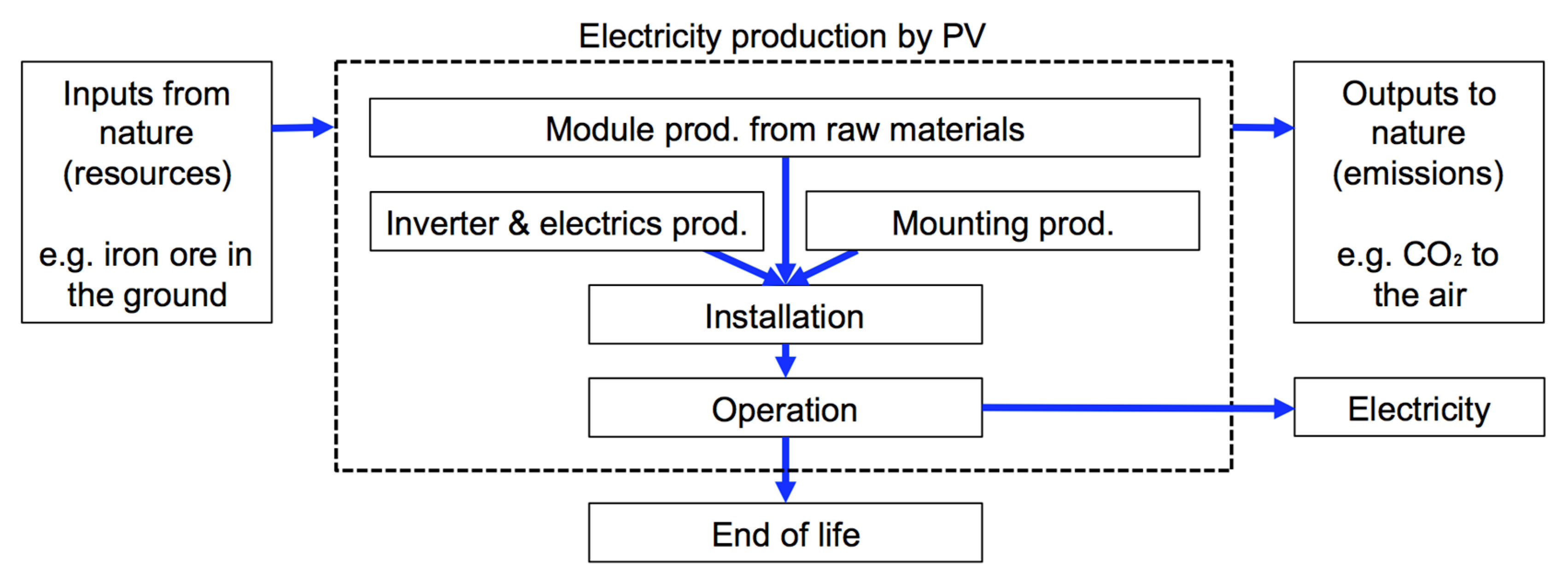
PV LCA-Goal, System Boundary, and Functional Unit

The goal is estimating the carbon intensity of PV power. The system is electricity production by PV. Electricity production can be considered a black box that consumes resources and produces electricity and emissions. The system’s primary function is producing electricity, and thus the functional unit is a kilowatthour of AC electricity supplied to the grid. In addition to electricity, the other system output we analyzed in the case study is GHG emissions. These two system outputs are combined into our central metric—GHGs emitted per AC electricity generated (gCO2e/kWh), or carbon intensity.
PV electricity production can be elaborated as shown in Figure 1 and Figure 2. Commercial thin film module production is relatively less complex and more vertically integrated [40,47], and is not further segmented beyond Figure 5. Crystalline silicon module production is further elaborated here, as shown in Figure 6.
LCA refers to the explicit stages in Figure 5 and Figure 6 as the “foreground” and their implied component processes as the “background”. Although not explicitly drawn, background processes are inside the system border and include the following: production of chemicals used in silicon processing; construction and operation of module-manufacturing infrastructure; and raw material extraction processes (e.g., iron ore acquisition) that “pull” resources from nature, across the system boundary, and into the electricity production system. In this analysis, transport is treated as a background process that contributes to multiple foreground stages. For example, chemicals are transported to the site of silicon processing. The processes not included in our system include the following: electricity transmission from generation site to end-use; displacement of competing power sources; and growth of a carbon-absorbing biomass underneath PV modules, which growth can be reduced by up to ~75% by module shading in temperate climates [48].

PV LCA-Data Sources

A list quantifying inputs and outputs of a stage is called a life cycle inventory (LCI). Our primary sources for PV foreground LCIs are the IEA’s 2015 Report “Life Cycle Inventories and Life Cycle Assessments of PV Systems” [41] and the 2012 Report “Life Cycle Inventories of Photovoltaics” by ESU-services [40]. These sources aggregate large numbers of LCIs and explicitly aim to represent production typical of the PV industry. The IEA report provides “mainstream” and “best technology” LCIs for Chinese mc-Si module production. We use the “mainstream” LCIs. Other sources for foreground LCIs are the Ecoinvent Database V3 [45] for an LCI of silica sand acquisition, and Sinha et al. [27] for an LCI of a horizontal one-axis tracking system. For emission factors of background processes, our primary data source is the Ecoinvent V3 database [45]. The impact assessment method used by Ecoinvent V3, and thus by our model, to calculate emission factors in units of CO2-equivalent is the Intergovernmental Panel on Climate Change’s 2013 GWP 100a method [49].
The referenced LCIs do not provide data on end of life (EOL), partly because the large majority of PVs installed have not reached their end of life. In the absence of data, our model does not account for emissions from PV EOL processes. Wind power LCAs face a similar lack of EOL data, but benefit from more established recycling processes for wind’s primary materials (steel from towers, fiber glass from blades, etc.).

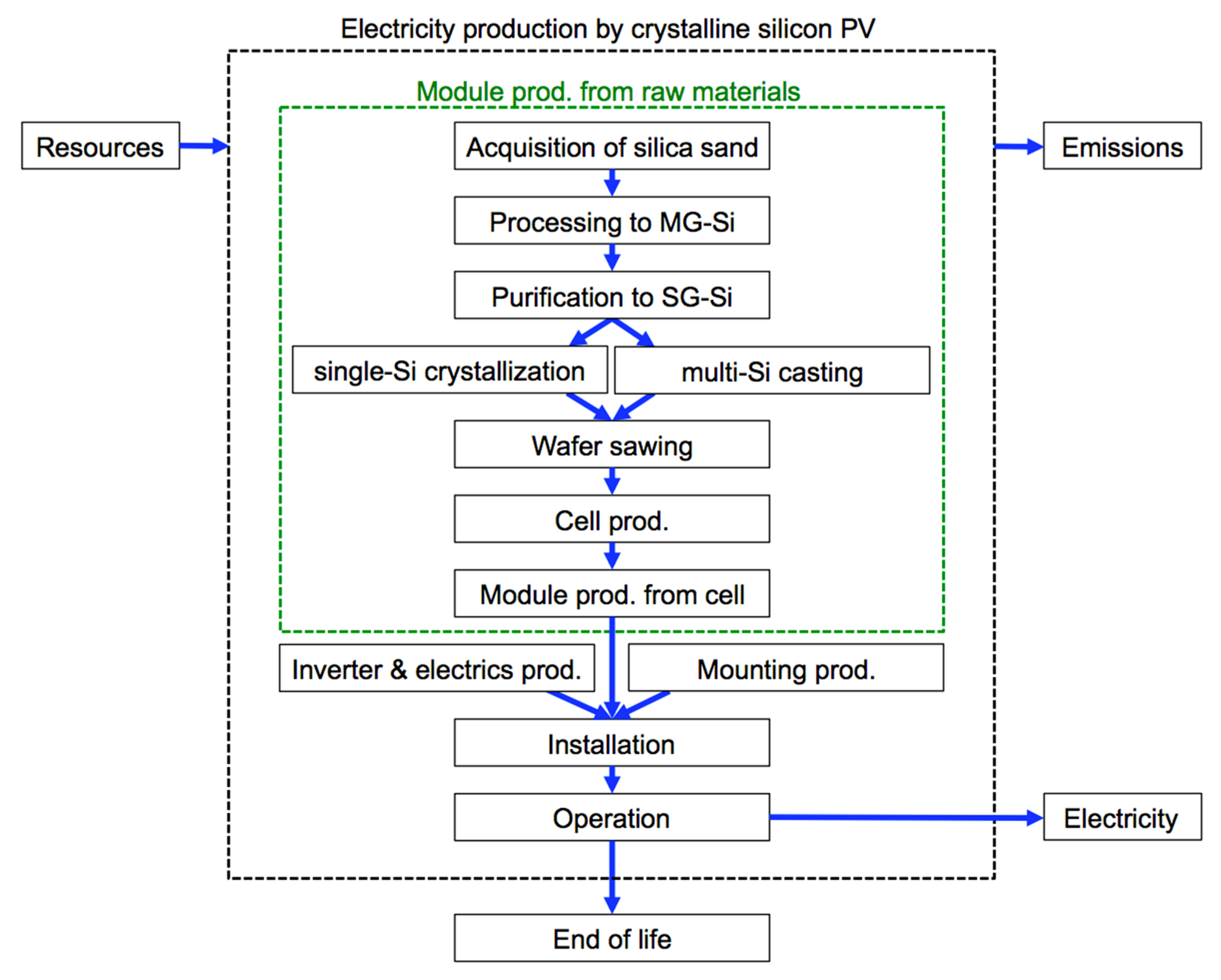
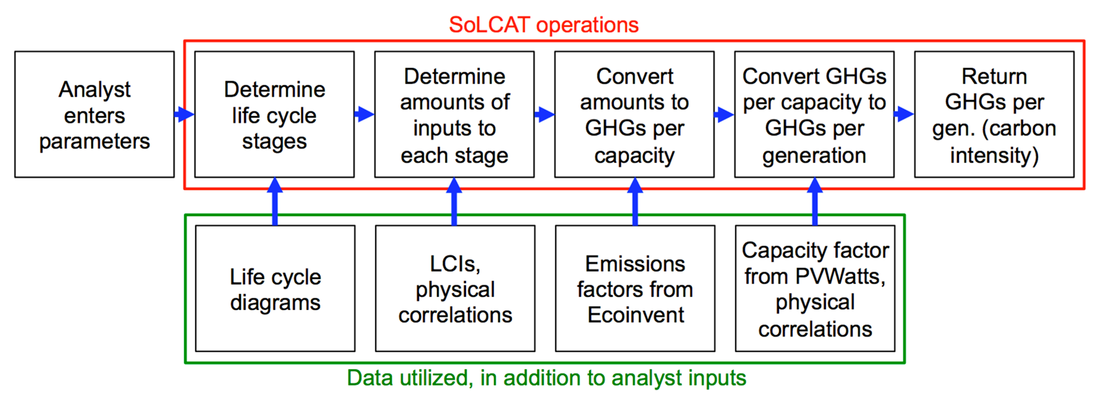
PV LCA-Model Structure

SoLCAT uses foreground LCIs and background emissions factors in several ways to estimate the carbon intensity of PV power. Figure 7 gives an overview of SoLCAT’s operation and utilization of data sources. Capacity refers to rated DC power capacity, unless otherwise indicated.
SoLCAT converts amounts ( a ) to GHG emissions ( e t o t a l ) using three general equations, shown below with indented examples after each equation, as follows:
e t o t a l = i e s t a g e   i
e t o t a l , m c S i = e S i s a n d   a c q u i s t i o n + e M G S i   p r o c e s s i n g + e c e l l   p r o d . + e i n s t a l l a t i o n + e o p e r a t i o n
e s t a g e   i = j e i n p u t   j   t o   s t a g e   i k s t a g e s   b e f o r e   i e s t a g e   k
e M G S i   p r o c e s s . = ( e c h a r c o a l   i n p u t   t o   M G S i   p r o c e s s . + e S i s a n d   i n p u t   t o   M G S i   p r o c e s s . + ) e S i s a n d   a c q .
e i n p u t   j   t o   s t a g e   i = a i n p u t   j   t o   s t a g e   i   E F j
e c h r o m i u m   s t e e l   i n p u t   t o   m o u n t i n g   p r o d . = a c h r o m i u m   s t e e l   i n p u t   t o   m o u n t i n g   p r o d .   E F c h r o m i u m   s t e e l
where e is emissions (gCO2e), a is amount (e.g., kg-iron, m3-acetone, etc.), and E F is emission factor (e.g., gCO2e/kg-iron, gCO2e/m3-acetone, etc.). Calculating the life cycle emissions for one scenario involves >100 variations of Equation (11) corresponding to different stages and inputs. Amounts ( a i n p u t   j   t o   s t a g e   i ) are provided by the PV LCIs [27,40,41,45] or are determined by input variables to SoLCAT. Emission factors ( E F j ) are provided by Ecoinvent [45] or SoLCAT inputs. Miller et al. [43] provide more detail on how SoLCAT utilizes the input variables impact amounts and emission factors.

PV LCA-Converting GHGs per Capacity to GHGs per Generation (Carbon Intensity)

SoLCAT’s last operation requires a capacity factor, or equivalently an energy yield. Our model utilizes capacity factor estimates from PVWatts [51]. PVWatts outputs a year-one DC capacity factor based on inputs of location, installation type, orientation, cell type, inverter loading ratio, rated inverter efficiency, ground coverage ratio, and system losses.
Our model adjusts capacity factors from PVWatts to account for shading, snow, light-induced degradation (LID), non-LID degradation (commonly called “degradation”), and tracker energy consumption, in order to calculate a lifetime average capacity factor ( F ). Finally, carbon intensity is calculated as follows:
I = e t o t a l / ( F c g t h r )
where I is carbon intensity (gCO2e/kWh), e t o t a l is life cycle GHG emissions (gCO2e), c g is rated power capacity, and t h r is PV system lifetime (h).

PV LCA-Tracking Energy Gain Methodology

An analysis of solar tracking’s impact on carbon intensity requires the calculation of tracking energy gain (TEG). TEG is the percentage increase in PV power output that results from tracking the sun, relative to a fixed-position system, and can be estimated using PVWatts as follows:
T E G = ( P ¯ A C , t r a c k P ¯ A C , f i x e d ) / P ¯ A C , f i x e d × 100 %
or equivalently
T E G = ( F t r a c k F f i x e d ) / F f i x e d × 100 %
where F t r a c k is the capacity factor of a PV system with tracking, and F f i x e d is the capacity factor of a PV system with fixed orientation but otherwise identical features (location, modules, etc.). When discussing TEG, the details of both the tracking system (whether one-axis or two-axis, axis of rotation, rotation limits, etc.) and the fixed base case (tilt and azimuth) should be specified. In this paper, the fixed base case orientation is always irradiance-maximizing, with equator-facing azimuth (south in the Northern Hemisphere anfd north in the Southern Hemisphere) and near-latitude tilt.

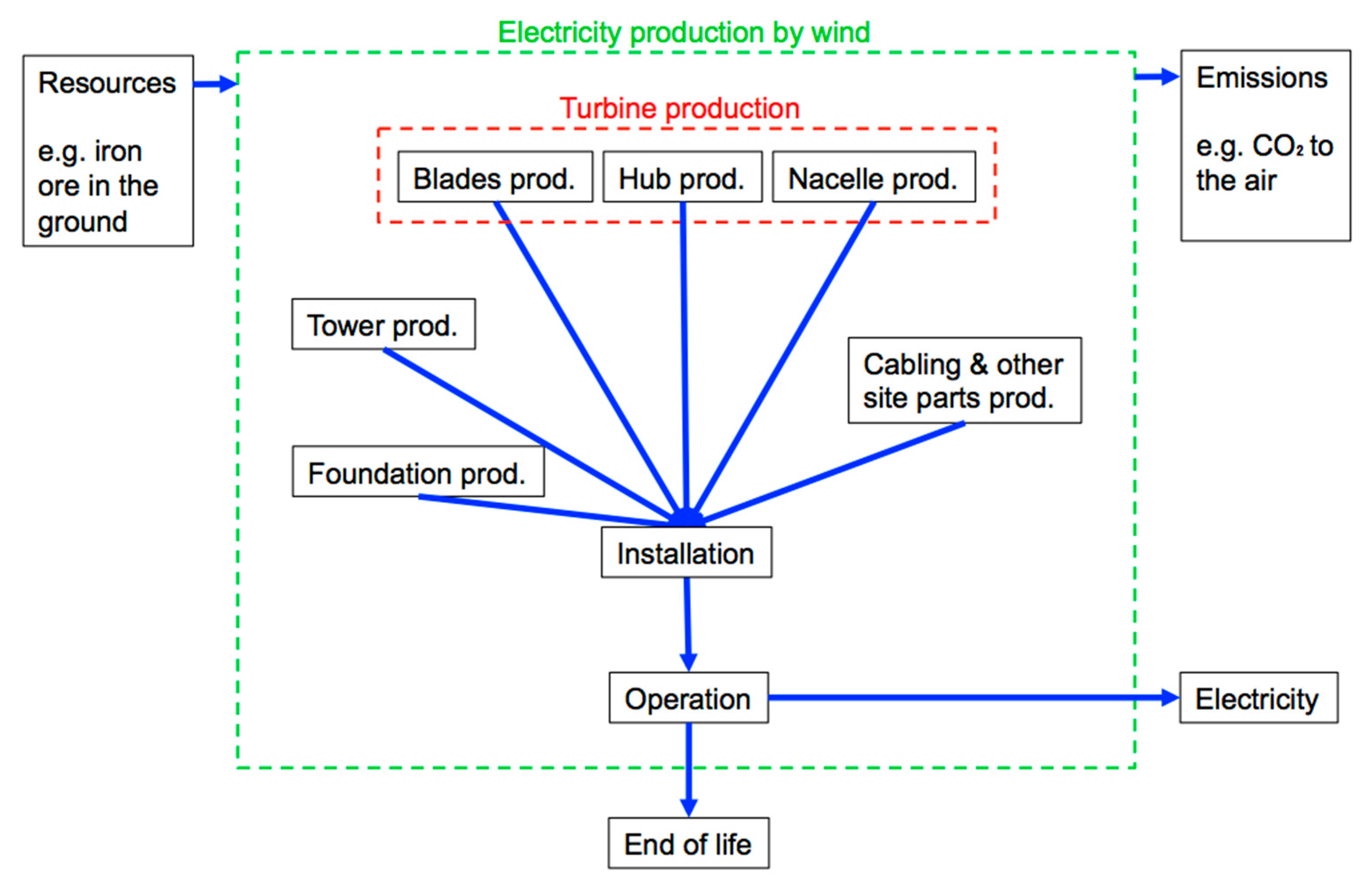
2.2.2. Wind LCA Synthesis

Wind electricity production can be elaborated as shown in Figure 8. To be consistent with our PV LCA, our wind system likewise excludes EOL and transmission from generation site to end-use.
Our main data sources are 10 wind power LCAs conducted by the turbine manufacturers Vestas and Siemens-Gamesa (also called SWP) in 2011–2017 [10,11,12,13,14,15,16,17,52,53]. Vestas and SWP together accounted for ~25% and ~50% of the new turbines installed in the world and in the United States, respectively, in 2016 [7,54]. SWP accounted for over half of both cumulative and new offshore installations in 2016 [7]. These LCAs have been reviewed for compliance with ISO 14040 LCA standards, by external reviewers in Vestas’ case and internal reviewers in SWP’s case. The 10 turbine types modeled are widely deployed in conditions matching our four categories of interest, namely: onshore low wind speed (~7 m/s), onshore medium (~8 m/s), onshore high (~9 m/s), and offshore high (~9 m/s). In the United States, four of the ten models are deployed in onshore low wind speed conditions, seven in onshore medium speed conditions, and five in onshore high speed conditions [8]. In Europe, three of ten are deployed in offshore high speed conditions [16,17,55].
Each LCA estimates the carbon intensity of generation from a “typical” wind farm of turbines of the modeled type. The definition of “typical” varies slightly across the 10 LCAs. Thus, before averaging the emissions figures in each of the four categories, we first harmonize several parameters. For example, we assume a distance to grid of 20 km for onshore wind farms [11]. If one LCA assumes 15 km to grid and emissions from grid cable production of 1 gCO2e/kWh, we multiply those emissions by 20 km/15 km = 1.33. We also harmonize lifetime (20 years), hub height (95 m), offshore distance to grid (70 km [7]), and hourly wind speed data (four data sets for four categories). The wind speed data are input into NREL’s System Advisor Model program, along with the turbine model, to estimate the capacity factors. Table 2 shows the results.

3. Results and Discussion

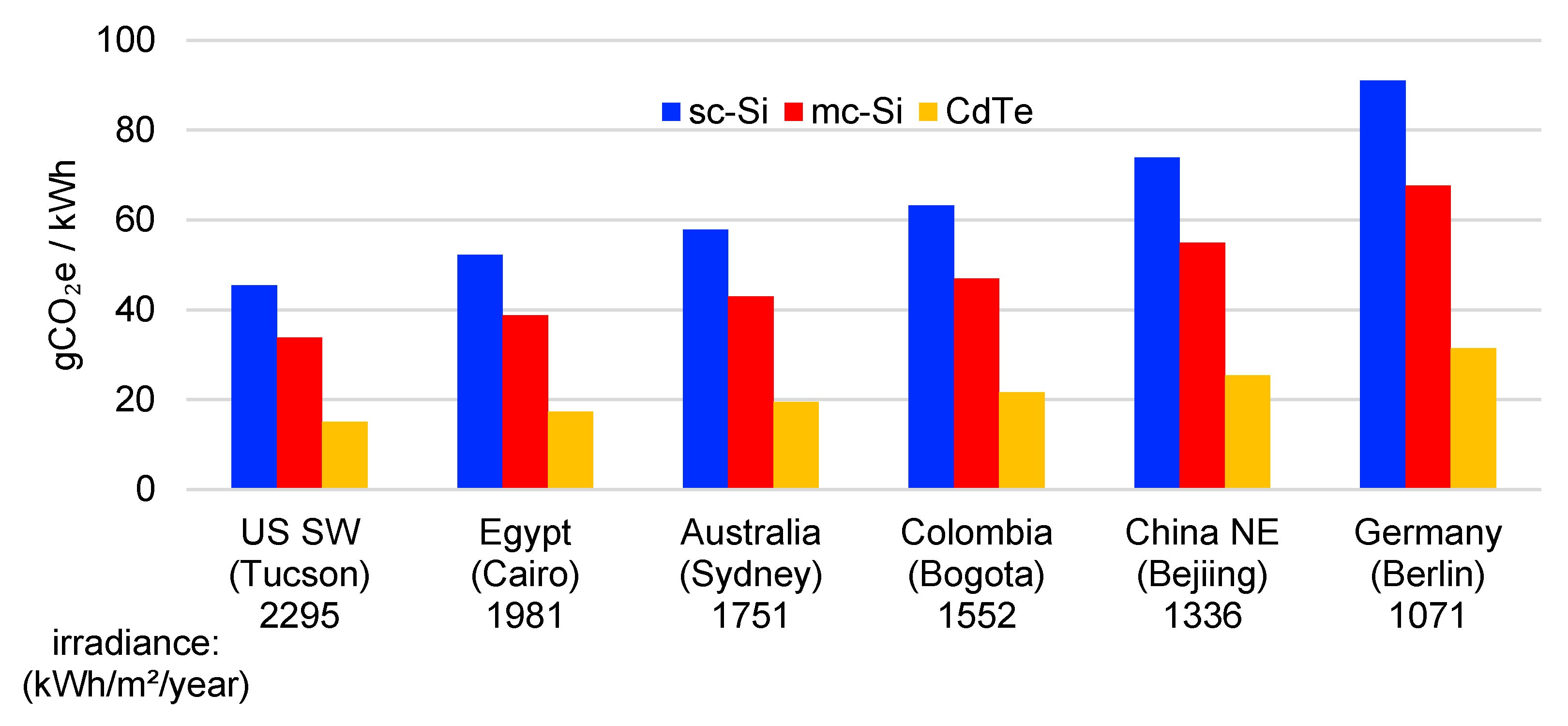
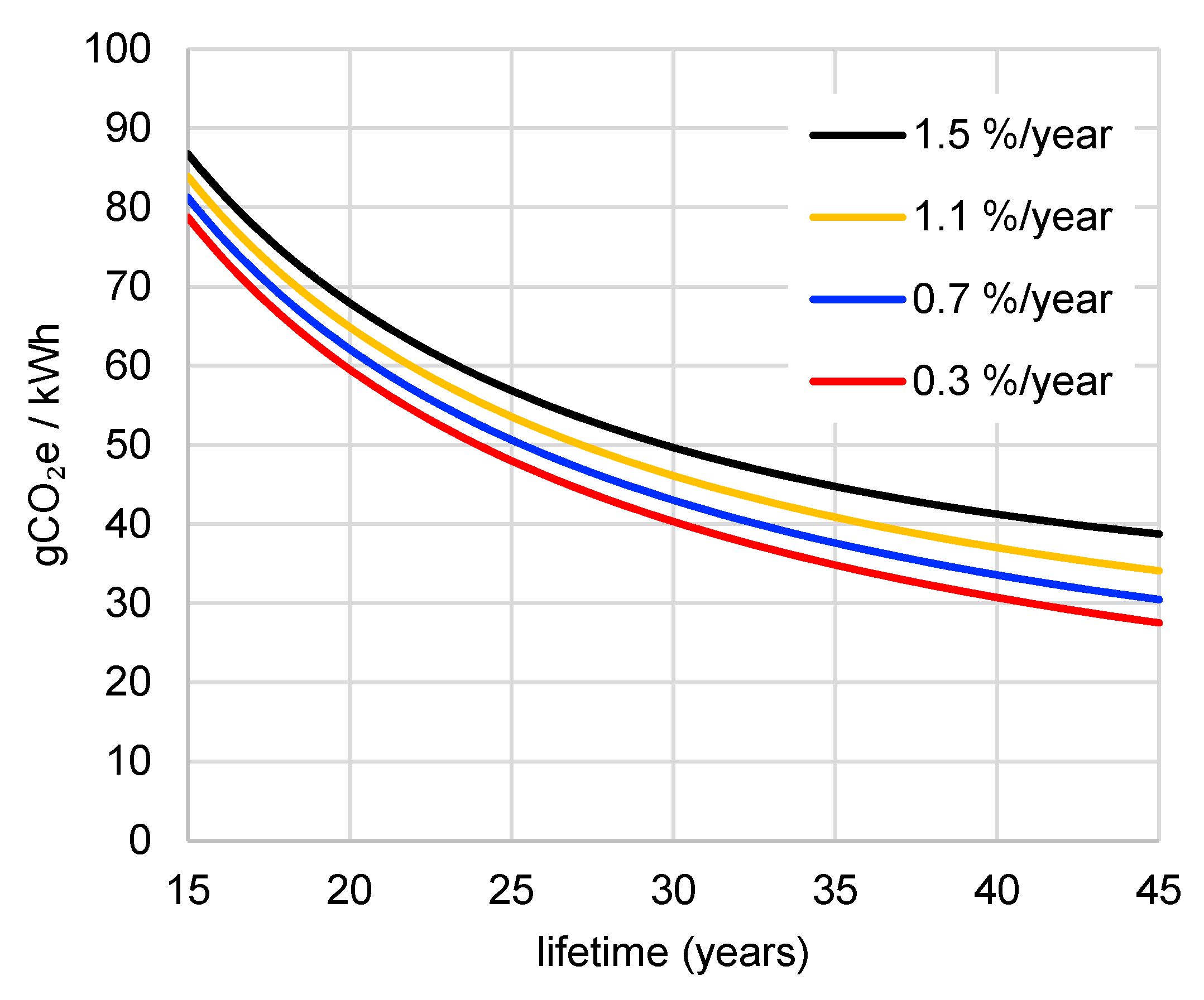
3.1. Base Cases for PV Generation (No Tracking, No Storage)

Figure 9 shows how PV carbon intensity varies by location, irradiance, and cell type. The parameter values used in Figure 9 are assumed throughout the paper, unless otherwise indicated. Figure 10 shows the sensitivity of PV carbon intensity to lifetime and degradation rate.

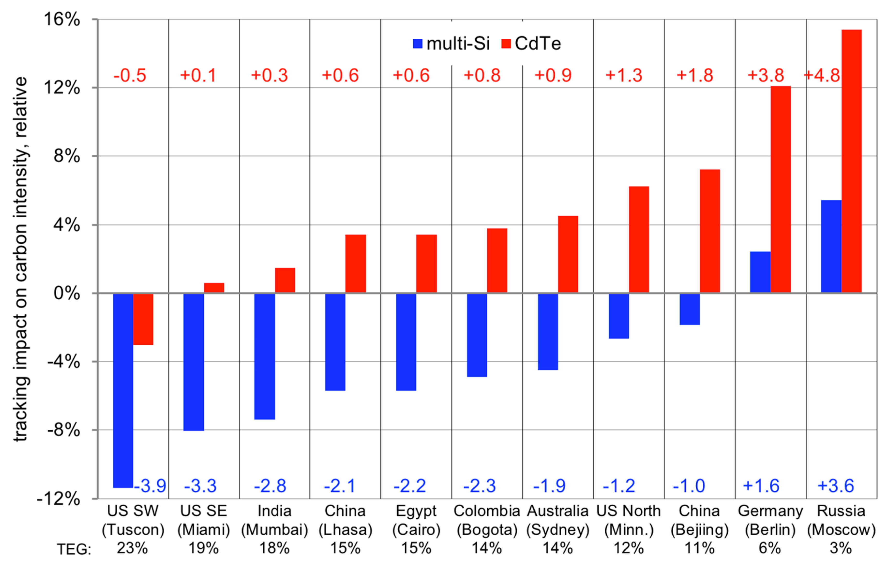
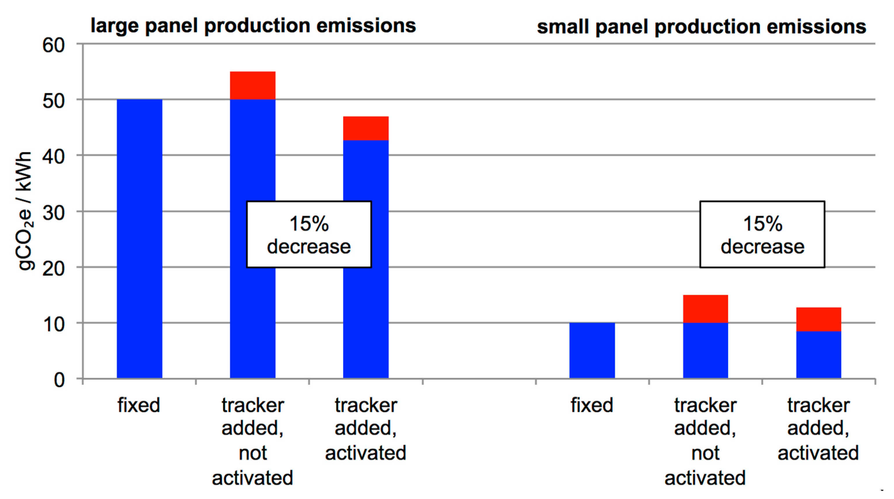
3.2. The Impact of Solar Tracking

We find that in the United States Southwest, for mc-Si PV, horizontal one-axis tracking reduces carbon intensity by 12% relative to the fixed-tilt base case (from 34 to 30 gC/kWh), consistent with previously published results [9]. Tracking produces this reduction despite requiring ~50% more structural metal (iron and aluminum) and ~30% more copper cable per module, compared to fixed-tilt mounting [27]. Emissions from producing extra tracker materials are offset by increased generation from tracking, such that the overall carbon intensity decreases.
To determine whether this ~10% emissions reduction holds for other regions and cell types, we applied analogous calculations to hypothetical mc-Si and CdTe PV systems at 10 other locations (the base cases from Figure 9), and have presented them in Figure 11, which underlines several related findings. (1) Location influences the emissions impact of tracking, via TEG; (2) tracking decreases the carbon intensity of mc-Si PV in most locations; (3) consistent with Sinha et al. [27], tracking reduces the carbon intensity of CdTe PV in the United States Southwest by ~3%; and (4) the United States Southwest is the exception to the rule—for most locations tested, tracking actually increases the carbon intensity of CdTe PV power. This includes many places with favorable economics for tracking and TEG above 13%. Near Sydney, Australia, for example, horizontal single-axis tracking increases both electricity output (by 14%) and carbon intensity (by 5%, from 19 to 20 gCO2e/kWh). In Germany, where tracking is less common, tracking increases power output by 6% and emissions by 13% (from 31 to 35 gCO2e/kWh).
The dependence on location is mainly driven by latitude and cloud cover. The greater the latitude, the greater the module tilt that maximizes incident irradiance, and the more irradiance is lost by “reclining” to a horizontal tilt for one-axis tracking (as described in Section 1, horizontal one-axis tracking is the norm for large-scale tracking; tilted one-axis trackers do exist, but are much less common for reasons including self-shading and wind concerns). Greater latitude also means more atmosphere for sunlight to travel through. This increases light scattering, as does greater cloud cover. The greater the fraction of ambient light that is scattered (i.e., diffuse), the less energy there is to be gained from tracking the sun’s non-diffuse direct beam irradiance. Lower tracking energy gain (TEG) means less extra electricity over which to amortize extra emissions from tracker-production. For both module types, this explains why, as TEG decreases left to right in Figure 11, tracking’s emissions impact increases in relative terms (the bars).
The varying impact by module type can be explained with the following equations:
Let:
T     the   factor   by   which   tracking   increases   electricity   generation .   E . g . ,   If   TEG = 20 % ,   T = 1.2 .
e f , i     emissions   of   fixed   PV   system   ( gCO 2 e ) .   i = mc-Si  or   CdTe
e t     emissions   from   adding   tracking   ( gCO 2 e )
E f     generation   from   fixed   PV   system   ( kWh )
E t     generation   from   tracking   PV   system   ( kWh )
I f     emissions   per   generation   ( carbon   intensity )   of   fixed   PV   system   ( gCO 2 e / kWh )
I t     emissions   per   generation   ( carbon   intensity )   of   tracking   PV   system   ( gCO 2 e / kWh )
M     factor   by   which   tracking   changes   carbon   intensity .
( M 1 ) × 100 % ,   the   percentage   by   which   tracking   changes   the   carbon   intensity .
Using these definitions,
M = I t / I f
= [ ( e f , i + e t ) / E t ] / [ e f , i / E f ]
= [ ( e f , i + e t ) / ( T × E f ) ] / [ e f , i / E f ]
M = ( e f , i + e t ) / ( T × e f , i )
Consider Equation (15) when e f , i e t , that is, when emissions from module production are much larger than emissions from tracker production, as follows:
M f   l a r g e = e f , i / ( T × e f , i )
M f   l a r g e = 1 / T
M f   l a r g e will always be less than 1, because T is always greater than 1. In other words, for a module type with large production emissions, adding tracking will reduce carbon intensity. This explains why adding tracking reduces the carbon intensity of mc-Si PV in most locations (blue bars in Figure 11). Multi-Si module production is significantly more carbon intensive than CdTe module production, as seen in Figure 6 and previously reported [41]. e f , m u l t i S i is approximately 11 × e t , whereas e f , C d T e is approximately 5 × e t . Equation (15) thus also explains why adding tracking increases CdTe PV’s carbon intensity in most locations (red bars in Figure 11), as follows:
M C d T e = ( e f , C d T e + e t ) / ( T × e f , C d T e )
( e f , C d T e + e f , C d T e / 5 ) / ( T × e f , C d T e )
M C d T e 1.2 / T
For M C d T e to be less than 1, T must be greater than 1.2. In other words, CdTe PV requires a TEG above 20% for tracking to reduce its carbon intensity, a TEG only possible in exceptionally sunny regions like the United States Southwest.
Figure 12 illustrates the general principle behind both scenarios (high- and low-module emissions). In the future, if the ratio of module production emissions to tracker production emissions increases, independent of absolute emission values, tracking will more commonly decrease PV carbon intensity.

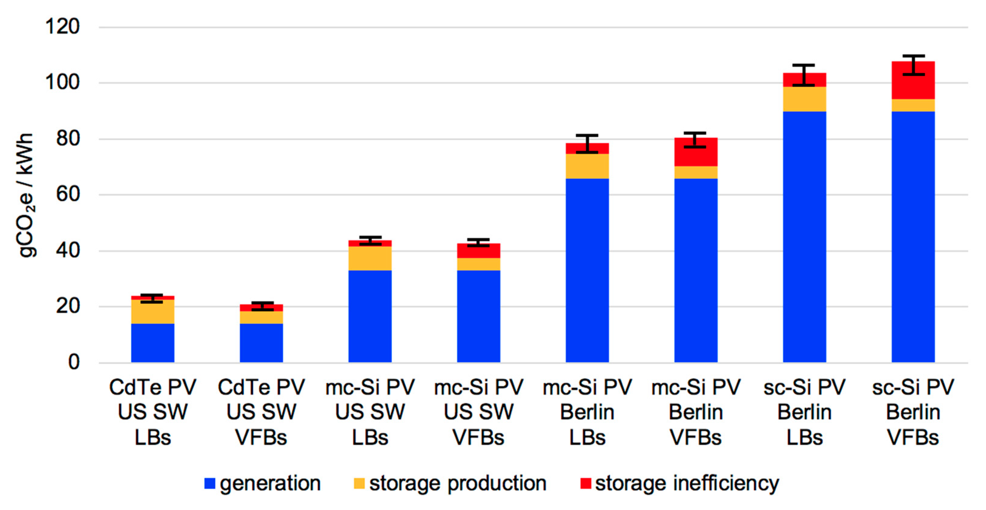
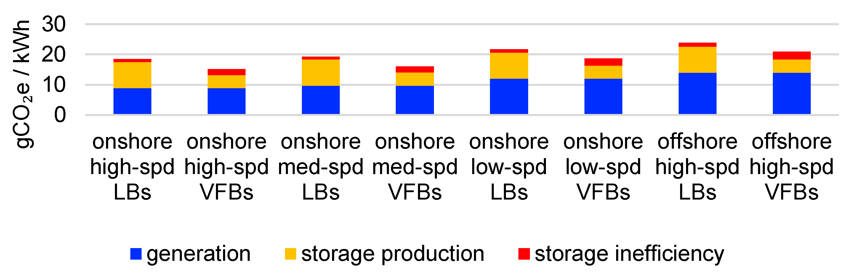
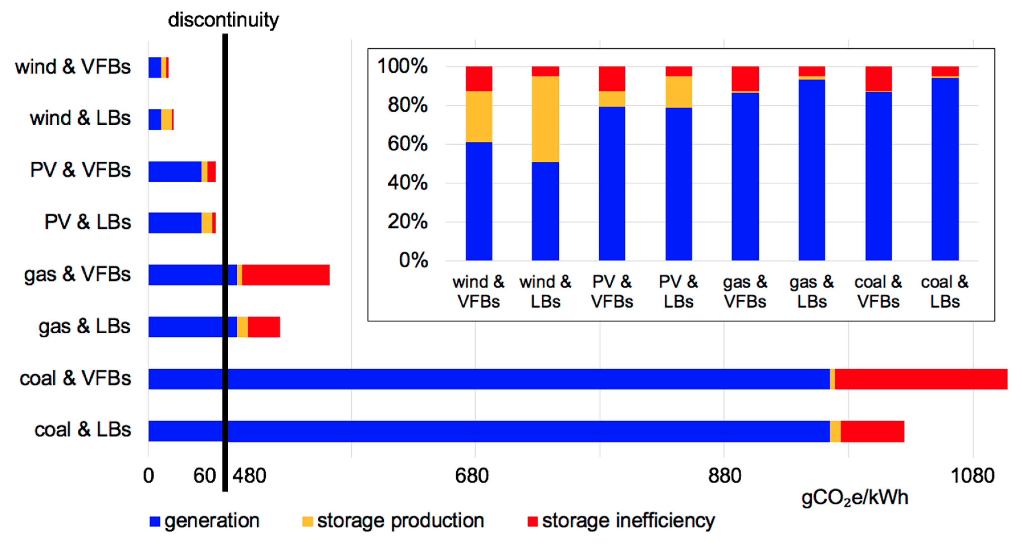
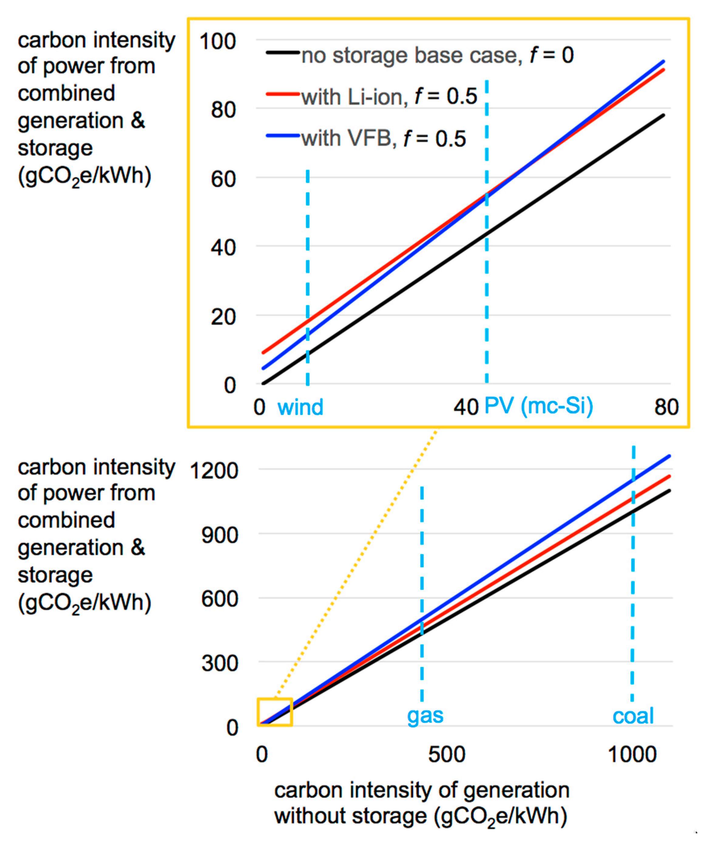
3.3. Hybrid Power Generation and Storage

Figure 13, Figure 14 and Figure 15 show the carbon intensity of electricity from coupled generation and batteries for PV, wind, and fossil-based generators, respectively. These carbon intensities are estimated using the model and LCAs described in Section 2. Figure 16 shows the linear correlation between coupled system carbon intensity and generator carbon intensity, and how storage technology affects that correlation.
The most important result is that, across all scenarios displayed, renewable electricity has much lower GHG emissions than fossil electricity. Figure 13, Figure 14, Figure 15 and Figure 16 show this to hold true, independent of renewable energy source, renewable power generation technology, location of generator, and integration of energy storage. As seen in Figure 13, the most carbon-intensive mainstream PV power (sc-Si PV produced in China, installed in Berlin, and coupled with sufficient LBs to store 50% of it’s generation) still emits only ~25% of the GHGs emitted by the least carbon intensive mainstream fossil power (CCNG with no storage). Therefore, to understand the GHG emissions impacts of renewables, future work should not focus on more accurately accounting for GHGs from the production of battery control systems or other system components. Whether wind power coupled with LBs emits 20 or 21 or even 40 gCO2e/kWh, it is still an order of magnitude less carbon intensive than fossil generation without carbon capture. Instead, future work on renewables’ emissions impacts should focus on consequential LCA, including questions of which generation types are most likely to be displaced by renewables deployment, dependent on location and economics, among other factors.
The percentage impact panel in Figure 15 illustrates another result—the storage parameter that controls emissions impact depends upon the generator to which the storage is coupled. Given low-emission generation, such as wind or CdTe PV, the storage feature that dominates emissions impact is storage production emissions (see orange sections in the left two bars of Figure 13). Given high-emission generation, such as gas or coal, the storage feature that dominates emissions impact is storage efficiency (see red sections in bottom four bars of Figure 15). One implication is that, if storage is being added to micro-grids or regional grids with low-emission generation (Iavg < 50 gCO2e/kWh), GHG emissions can be minimized by deploying storage products with the lowest production emissions. Conversely, if storage is being added to regions with high-emission generation (Iavg > 200 gCO2e/kWh), GHG emissions can be minimized by deploying storage products with the highest efficiency.
Figure 16 illustrates the linear relationship between the coupled system carbon intensity and generator carbon intensity. The parameters of the storage technology influence both the y-axis intersection and the slope of the line, according to the model equations in Section 2.1, as follows:
y a x i s   i n t e r s e c t i o n = η ( e s / E s T ) / ( D C ) / ( 1 / f 1 + η )
s l o p e = [ 1 f ( 1 η ) ]
These values are not particular to GHGs. Analogous qualitative behavior will thus hold for emissions of other pollutants, as well as “emissions” of dollars (costs/kWh). That is, emission and cost intensities of coupled systems, as a function of generator intensity, will have different slopes dependent on storage technology. Choosing a specific storage technology for a coupled system can minimize emissions (or cost) intensity for one generator, but not for another.

4. Conclusions

A model for estimating emissions from integrated power generation and energy storage is presented. The model applies to the emissions of all pollutants, including greenhouse gases (GHGs), and to all storage technologies, including pumped hydroelectric and electrochemical storage. As a case study, the model is used to estimate the GHG emissions of electricity from systems that couple photovoltaic and wind generation with lithium-ion batteries (LBs) and vanadium redox flow batteries (VFBs). To facilitate the case study, we conduct a life cycle assessment (LCA) of photovoltaic (PV) power, and a synthesis of existing wind power LCAs. The PV LCA is also used to estimate the emissions impact of a common PV practice that has not been comprehensively analyzed by LCA—solar tracking. Relative to stationary mounting, solar tracking is found to decrease the GHG emissions of power from multi-crystalline silicon PV in most of the regions analyzed (by 0 to ~12%, or 0 to ~4 gCO2e/kWh), and to increase the emissions of power from cadmium telluride PV in most regions analyzed (by 0 to ~12%, or 0 to ~4 gCO2e/kWh). For either PV cell type, if the ratio of module production emissions to tracker production emissions increases in the future, independent of absolute emission values, tracking will more commonly decrease PV carbon intensity. The case study of renewables and battery storage indicates that PV and wind power remain much less carbon intensive than fossil-based generation, even when coupled with large amounts of LBs or VFBs. The most carbon intensive renewable power analyzed (single-crystalline silicon PV produced in China, installed in Berlin, and coupled with sufficient VFBs to store 50% of it’s generation) still emits only ~25% of the GHGs of the least carbon intensive mainstream fossil power (combined cycle natural gas turbine with no storage). Lastly, we find that the pathway to minimize GHG emissions of power from a coupled system depends upon the generator—given low-emission generation (<50 gCO2e/kWh), the minimizing pathway is the storage technology with lowest production emissions (VFBs over LBs for our case study), and given high-emission generation (>200 gCO2e/kWh), the minimizing pathway is the storage technology with highest round-trip efficiency (LBs over VFBs). The latter case applies to a majority of the world’s power generation today. Directions for future work include the application of the coupled storage and generation model to other non-battery technologies, including pumped hydroelectric storage.

Author Contributions

I.M., E.G., and F.M.O. designed the research; I.M and E.G. developed the models and derived equations; I.M. performed all systems calculations; I.M., E.G., and F.M.O. analyzed data; I.M. and E.G. drafted the manuscript; all authors reviewed, edited, and approved the final version of the manuscript. F.M.O. directed the overall research.

Funding

This research was supported by The Low Carbon Energy Centers of the MIT Energy Initiative.

Conflicts of Interest

The authors declare no conflict of interest.

Nomenclature (In Order of Appearance)

GHGgreenhouse gas
IEAInternational Energy Agency
PVphotovoltaic
mc-Simulti-crystalline silicon
sc-Sisingle-crystalline silicon
CdTecadmium telluride
gCO2egrams CO2 equivalent
CCNGcombined cycle natural gas
SCPCsupercritical pulverized coal
cradle-to-gravecovering all parts of a product’s life cycle from raw material acquistion (cradle) through disposal and/or recycling (grave)
cradle-to-gatecovering all parts of a product’s life cycle from raw material acquistion (cradle) through production (factory gate)
LCAlife cycle assessment
utility-scalehaving AC capacity >5 MW, used to describe power plants
LBlithium-ion battery
VFBvanadium redox flow battery
LABlead acid battery
SSBsodium sulfur battery
PHSpumped hydroelectric storage
CAEScompressed air energy storage
P0power generation (kW)
Ppower supply to grid (kW)
Ps,inis the amount of power generation sent to storage (kW)
sis the instantaneous fraction of power generation going to storage
Ps,outis the power supply to grid from storage
ηround-trip efficiency of the storage
f the fraction of energy generation sent to storage (vs. directly to grid)
Elifetime electricity supply to grid from power plant (kWh)
E0lifetime electricity supply to grid from power plant without storage (kWh)
Iemissions intensity (g/kWh)
e g the life emissions of the generator (g)
e s the life emissions of the storage (g)
D ¯ or DoDthe average depth of discharge of the storage (DoD)
E s T the total rated energy capacity of storage used over the power plant life (kWh)
C the cycle life of the storage (the number of charge–discharge cycles before a storage unit is retired)
m s the mass of batteries used over the power plant life (kg)
ρ the specific energy capacity of the batteries (kWh/kg)
E s T the total rated energy capacity of all storage used and retired over the power plant life
cgrated power capacity
Fcapacity factor
TEGtracking energy gain
EOLend of life

References

  1. IEA. Energy, Climate Change & Environment; IEA: Paris, France, 2016. [Google Scholar]
  2. The Energy Initiative MIT. The Future of Solar Energy: An Interdiscipinary MIT Stud; MIT: Cambridge, MA, USA, 2015; pp. 3–6. [Google Scholar] [CrossRef]
  3. GlobalData. Solar PV Generation Statistics, Wind Generation Statistics; GlobalData: London, UK, 2018. [Google Scholar]
  4. ExxonMobil. 2017 Outlook for Energy: A View to 2040; ExxonMobil: Irving, TX, USA, 2017. [Google Scholar]
  5. BNEF. Bloomberg New Energy Finance Report 2017; BNEF: New York, NY, USA, 2017. [Google Scholar]
  6. Fraunhofer Institute for Solar Energy Systems. Photovoltaics Report; Fraunhofer Institute for Solar Energy Systems: Freiburg, Germany, 2017. [Google Scholar]
  7. WindEurope. The European Offshore Wind Industry—Key Trends And Statistics 2017; WindEurope: Brussels, Belgium, 2018. [Google Scholar]
  8. EIA. Form EIA-860: Annual Electric Generator Report; EIA: Paris, France, 2016. [Google Scholar]
  9. Leccisi, E.; Raugei, M.; Fthenakis, V. The energy and environmental performance of ground-mounted photovoltaic systems—A timely update. Energies 2016, 9, 622. [Google Scholar] [CrossRef]
  10. Garrett, P.; Rønde, K. Life Cycle Assessment of Electricity Production from an Onshore V90-3.0 MW Wind Plant September 2012; Vestas Wind Systems A/S: Aarhus, Denmark, 2012; pp. 1–106. [Google Scholar]
  11. Garrett, P.; Rønde, K.; Finkbeiner, M. Life Cycle Assessment of Electricity Production from an Onshore V110-2.0 MW Wind Plant; Vestas Wind Systems A/S: Aarhus, Denmark, 2012; pp. 1–106. [Google Scholar]
  12. Garrett, P.; Klaus, R. Life Cycle Assessment of Electricity Production from a V100-1.8 MW Gridstreamer Wind Plant; Vestas Wind Systems A/S: Aarhus, Denmark, 2011; p. 105. [Google Scholar]
  13. Razdan, A.P.; Garrett, P. Life Cycle Assessment of Electricity Production from an Onshore V100-2.0 MW Wind Plant; Vestas Wind Systems A/S: Aarhus, Denmark, 2015. [Google Scholar]
  14. Siemens. Onshore Wind Power Plant Employing SWT-2.3-108. In A Clean Energy Solut—From Cradle to Grave; Siemens: Munich, Germany, 2014; 16p. [Google Scholar]
  15. Siemens. Onshore Wind Power Plant Employing SWT-3.2-113. In A Clean Energy Solut—From Cradle to Grave; Siemens: Munich, Germany, 2014; 16p. [Google Scholar]
  16. Siemens. Offshore Wind Power Plant Employing SWT-4.0-130. In A Clean Energy Solut—From Cradle to Grave; Siemens: Munich, Germany, 2014; 16p. [Google Scholar]
  17. Siemens. Offshore Wind Power Plant Employing SWT-7.0-154. In A Clean Energy Solut—From Cradle to Grave; Siemens: Munich, Germany, 2014; 16p. [Google Scholar]
  18. Weinzettel, J.; Reenaas, M.; Solli, C.; Hertwich, E.G. Life cycle assessment of a floating offshore wind turbine. Renew. Energy 2009, 34, 742–747. [Google Scholar] [CrossRef]
  19. Skone, T.J.; Littefield, J.; Cooney, G.; Marriott, J. Power Generation Technology Comparison from a Life Cycle Perspective; National Energy Technology Laboratory: Pittsburgh, PA, USA, 2013.
  20. Peng, J.; Lu, L.; Yang, H. Review on life cycle assessment of energy payback and greenhouse gas emission of solar photovoltaic systems. Renew. Sustain. Energy Rev. 2013, 19, 255–274. [Google Scholar] [CrossRef]
  21. Hsu, D.D.; O’Donoughue, P.; Fthenakis, V.; Heath, G.A.; Kim, H.C.; Sawyer, P.; Choi, J.K.; Turney, D.E. Life Cycle Greenhouse Gas Emissions of Crystalline Silicon Photovoltaic Electricity Generation: Systematic Review and Harmonization. J. Ind. Ecol. 2012, 16, S122–S135. [Google Scholar] [CrossRef]
  22. Frischknecht, R.; Heath, G.; Raugei, M.; Sinha, P.; de Wild-Scholten, M.; Fthenakis, V. Methodology Guidelines on Life Cycle Assessment of Photovoltaic Electricity, 3rd ed.; IEA PVPS Task 12; National Renewable Energy Lab. (NREL): Golden, CO, USA, 2016.
  23. Bayod-Rújula, Á.A.; Lorente-Lafuente, A.M.; Cirez-Oto, F. Environmental assessment of grid connected photovoltaic plants with 2-axis tracking versus fixed modules systems. Energy 2011, 36, 3148–3158. [Google Scholar] [CrossRef]
  24. Desideri, U.; Zepparelli, F.; Morettini, V.; Garroni, E. Comparative analysis of concentrating solar power and photovoltaic technologies: Technical and environmental evaluations. Appl. Energy 2013, 102, 765–784. [Google Scholar] [CrossRef]
  25. Beylot, A.; Payet, J.Ô.; Puech, C.; Adra, N.; Jacquin, P.; Blanc, I.; Beloin-Saint-Pierre, D. Environmental impacts of large-scale grid-connected ground-mounted PV installations. Renew. Energy 2014, 61, 2–6. [Google Scholar] [CrossRef] [Green Version]
  26. Bolinger, M.; Seel, J.; La Commare, K.H. Utility-Scale Solar 2016; LBNL-2001055; Lawrence Berkeley National Laboratory: Foshan, Guangdong, China, September 2017.
  27. Sinha, P.; Schneider, M.; Dailey, S.; Jepson, C.; De Wild-Scholten, M. Eco-efficiency of CdTe photovoltaics with tracking systems. In Proceedings of the 39th IEEE Photovoltaic Specialists Conference (PVSC), Tampa, FL, USA, 16–21 June 2013. [Google Scholar]
  28. Sivaram, V.; Kann, S. Solar power needs a more ambitious cost target. Nat. Energy 2016, 1, 16036. [Google Scholar] [CrossRef]
  29. Zhuk, A.; Zeigarnik, Y.; Buzoverov, E.; Sheindlin, A. Managing peak loads in energy grids: Comparative economic analysis. Energy Policy 2016, 88, 39–44. [Google Scholar] [CrossRef]
  30. Krieger, E.M.; Casey, J.A.; Shonkoff, S.B.C. A framework for siting and dispatch of emerging energy resources to realize environmental and health benefits: Case study on peaker power plant displacement. Energy Policy 2016, 96, 302–313. [Google Scholar] [CrossRef]
  31. Denholm, P.; Hand, M. Grid flexibility and storage required to achieve very high penetration of variable renewable electricity. Energy Policy 2011, 39, 1817–1830. [Google Scholar] [CrossRef]
  32. Simon, B.; Finn-Foley, D.; Gupta, D. GTM Research/ESA U.S. Energy Storage Monitor; GTM: Boston, MA, USA, 2018. [Google Scholar]
  33. Yang, G. Is this the ultimate grid battery? IEEE Spectrum 2017, 54, 36–41. [Google Scholar] [CrossRef]
  34. Spanos, C.; Turney, D.E.; Fthenakis, V. Life-cycle analysis of flow-assisted nickel zinc-, manganese dioxide-, and valve-regulated lead-acid batteries designed for demand-charge reduction. Renew. Sustain. Energy Rev. 2015, 43, 478–494. [Google Scholar] [CrossRef]
  35. Rydh, C.J.; Sandén, B.A. Energy analysis of batteries in photovoltaic systems. Part I: Performance and energy requirements. Energy Convers. Manag. 2005, 46, 1957–1979. [Google Scholar] [CrossRef]
  36. Denholm, P.; Kulcinski, G.L. Life cycle energy requirements and greenhouse gas emissions from large scale energy storage systems. Energy Convers. Manag. 2004, 45, 2153–2172. [Google Scholar] [CrossRef]
  37. Mitavachan, H.; Derendorf, K.; Vogt, T. Comparative life cycle assessment of battery storage systems for stationary applications. Environ. Sci. Technol. 2015. [Google Scholar] [CrossRef]
  38. Cui, Y.; Du, C.; Yin, G.; Gao, Y.; Zhang, L.; Guan, T.; Yang, L.; Wang, F. Multi-stress factor model for cycle lifetime prediction of lithium ion batteries with shallow-depth discharge. J. Power Source 2015, 279, 123–132. [Google Scholar] [CrossRef]
  39. Alsaidan, I.; Khodaei, A.; Gao, W. A Comprehensive Battery Energy Storage Optimal Sizing Model for Microgrid Applications. IEEE Trans. Power Syst. 2018, 33, 3968–3980. [Google Scholar] [CrossRef]
  40. Jungbluth, N.; Stucki, M.; Flury, K.; Frischknecht, R.; Büsser, S. Life Cycle Inventories of Photovoltaics; ESU-services Ltd.: Ulster, Switzerland, 2012. [Google Scholar]
  41. Frischknecht, R.; Itten, R.; Sinha, P.; de Wild-Scholten, M.; Zhang, J.; Fthenakis, V. Life Cycle Inventories and Life Cycle Assessment of Photovoltaic Systems; Report IEA-PVPS T12-04:2015; International Energy Agency (IEA): Paris, France, 2015. [Google Scholar]
  42. Eaton, C.T. AC vs. DC Coupling in Utility-Scale Solar Plus Storage Projects; Eaton: Cleveland, OH, USA, 2016. [Google Scholar]
  43. Miller, I.; Gençer, E.; Vogelbaum, H.S.; Brown, P.R.; Torkamani, S.; O’Sullivan, F.M. Parametric modeling of life cycle greenhouse gas emissions from photovol-taic power. Appl. Energy 2018. Under Review. [Google Scholar]
  44. ISO 14040. The International Standards Organisation. Environmental Management—Life cycle Assessment—Principles and Framework; ISO 14040 2006; ISO: Geneva, Switzerland, 2006; pp. 1–28. [Google Scholar] [CrossRef]
  45. Steubing, B.; Wernet, G.; Reinhard, J.; Bauer, C.; Moreno-Ruiz, E. The ecoinvent database version 3 (part II): Analyzing LCA results and comparison to version 2. Int. J. Life Cycle Assess. 2016, 21, 1269–1281. [Google Scholar] [CrossRef]
  46. Gagnon, P.; Margolis, R.; Melius, J.; Phillips, C.; Elmore, R. Rooftop Solar Photovolatic Technical Potential in the United States: A Detailed Assessment; National Renewable Energy Lab.(NREL): Golden, CO, USA, 2016; p. 82. [CrossRef]
  47. Jean, J.; Brown, P.R.; Jaffe, R.L.; Buonassisi, T.; Bulović, V. Pathways for solar photovoltaics. Energy Environ. Sci. 2015, 8, 1200–1219. [Google Scholar] [CrossRef]
  48. Gençer, E.; Miskin, C.; Sun, X.; Khan, M.R.; Bermel, P.; Alam, M.A.; Agrawal, R. Directing solar photons to sustainably meet food, energy, and water needs. Sci. Rep. 2017, 7, 3133. [Google Scholar] [CrossRef] [PubMed]
  49. Pachauri, R.K.; Allen, M.R.; Barros, V.R.; Broome, J.; Cramer, W.; Christ, R.; Church, J.A.; Clarke, L.; Dahe, Q.; Dasgupta, P. Climate Change 2014: Synthesis Report; Contribution of Working Groups, I II and III to the Fifth Assessment Report of the Intergovernmental Panel on Climate Change; IPCC: Geneva, Switzerland, 2014. [Google Scholar] [CrossRef]
  50. Gilman, P.; Dobos, A.; DiOrio, N.; Freeman, J.; Janzou, S.; Ryberg, D. SAM Photovoltaic Model Technical Reference Update; NREL: Golden, CO, USA, 2018.
  51. Dobos, A.P. PVWatts Version 5 Manual; NREL/TP-6A20-62641; National Renewable Energy Lab. (NREL): Golden, CO, USA, 2014.
  52. Garrett, P.; Ronde, K. Life Cycle Assessment of Electricity Production from an Onshore V90-2.6 MW Wind Plant; Vestas Wind Systems A/S: Aarhus, Denmark, 2013; p. 107. [Google Scholar]
  53. Razdan, A.P.; Garrett, P. December 2015 Life Cycle Assessment of Electricity Production from an Onshore V110-2.0 MW Wind Plant; Vestas Wind Systems A/S: Aarhus, Denmark, 2015. [Google Scholar]
  54. GWEC. Global Wind Statistics 2016; GWEC: Brussels, Beligum, 2017. [Google Scholar]
  55. Siemens. Offshore wind power plant employing SWT-6.0-154. In A Clean Energy Solut—From Cradle to Grave; Siemens: Munich, Germany, 2014; 16p. [Google Scholar]
  56. Jordan, D.C.; Kurtz, S.R.; VanSant, K.; Newmiller, J. Compendium of photovoltaic degradation rates. Prog. Photovolt. Res. Appl. 2016, 24, 978–989. [Google Scholar] [CrossRef]
  57. IEA. CO2 Emissions from Fuel Combustion 2017; International Energy Agency: Paris, France, 2017. [Google Scholar] [CrossRef]
Figure 1. Three scenarios corresponding to three times of day for a combined photovoltaic (PV) and storage system. P0 is power generation (kW), P is power supply to grid (kW), Ps,in is the amount of power generation sent to storage (kW), s is the instantaneous fraction of power generation going to storage, and Ps,out is the power supply to grid from storage.
Processes 06 00267 g001
Figure 2. Average power flows of combined generation and storage. Over-bars indicate time averages, η is the round-trip efficiency of the storage, and f is the fraction of energy generation sent to storage (vs. directly to grid).
Processes 06 00267 g002
Figure 3. Dependence of f (fraction of generation sent to storage) on power generation and supply curves. Assumes no curtailment.
Processes 06 00267 g003
Figure 4. Life cycle stages of battery production.
Processes 06 00267 g004
Figure 5. Life cycle stages of PV electricity production.
Processes 06 00267 g005
Figure 6. Life cycle stages of electricity production by crystalline silicon PV (MG-Si: metallurgical grade silicon; SG-Si: solar grade silicon).
Processes 06 00267 g006
Figure 7. Flowchart of SoLCAT operations and utilization of data sources. Capacity is rated DC capacity. Generation is AC electricity generation (SoLCAT: solar life cycle assessment tool; GHGs: greenhouse gas; LCIs: life cycle inventories).
Processes 06 00267 g007
Figure 8. Life cycle stages of wind electricity production.
Processes 06 00267 g008
Figure 9. Carbon intensities of power from PV power plants installed in different locations around 2015. Installation type is large-scale (AC capacity >1 MW), open-ground, and fixed. Irradiance is lifetime-average irradiance incident on modules. Lifetime is 30 years. Rated module efficiencies are 17%, 16%, and 15.6% for sc-Si, mc-Si, and CdTe, respectively [9]. Degradation is 0.7%/year [56]. GHG emissions of upstream electricity are 660 gCO2e/kWh for module production and 510 for balance of system (BOS) production, corresponding to Chinese and global averages in 2015 [57]. These parameter values are assumed throughout the paper, unless otherwise indicated.
Processes 06 00267 g009
Figure 10. Carbon intensity of mc-Si PV power vs. lifetime at different degradation rates. Location is Sydney, Australia. Rated module efficiency is 16%. Other parameters match values in Figure 9.
Processes 06 00267 g010
Figure 11. The impact of horizontal one-axis solar tracking on PV carbon intensity in different locations, for mc-Si PV (blue), and CdTe PV (red). The y-axis and bars indicate relative impact, that is, percentage change in carbon intensity compared to fixed PV at the same location: Percentage change = ( C I t r a c k i n g   P V C I f i x e d   P V ) / C I f i x e d   P V × 100 % . The red and blue numbers indicate the absolute impact (gCO2e/kWh): absolute change = ( C I t r a c k i n g   P V C I f i x e d   P V ). Tracking energy gains (TEGs) are at the bottom.
Processes 06 00267 g011
Figure 12. Illustration of how panel production emissions influence whether tracking decreases (left) or increases (right) the carbon intensity, relative to the fixed PV. Left and right systems have the same location and power output per panel. Activating tracking on both boosts power by 17%, a typical TEG for a sunny location. Red represents the tracker contribution to emissions. In terms of Equation (15) definitions, red represents e t / g f in the “not activated” bars, and e t / g t in the “activated” bars. Emissions values in this figure are arbitrary and chosen to illustrate the concept. A TEG of 17% is assumed, giving a 15% reduction in carbon intensity upon activation.
Processes 06 00267 g012
Figure 13. GHG emissions of power from different PV systems coupled with LBs or VFBs. PV systems differ by cell type and installation location. Other parameters match base case values in Figure 9. Bars indicate the difference between “best” and “worst” case scenarios for each storage technology. Best assumes the high values of efficiency and cycle life in Section 2.1.2, while worst assumes the low values. Fraction of generation sent to storage f is 50%, to correspond to the approximate upper bound of f needed to flatten the intermittent generation, or conversely needed to convert constant fossil-based generation into peak supply (CdTe: cadmium telluride; mc-Si: multi-crystalline silicon; sc-Si: single-cyrstalline silicon; LBs: lithium-ion batteries; VFBs: vanadium redox flow batteries).
Processes 06 00267 g013
Figure 14. GHG emissions of power from different wind power systems coupled with LBs or VFBs. Wind systems differ by average local wind-speed and installation onshore or offshore. Other parameters match assumptions in Table 2. Bars indicate the difference between “best” and “worst” case scenarios for each storage technology. Best assumes the high values of efficiency and cycle life in Table 2, while worst assumes the low values. The fraction of generation sent to storage f is 50%, to correspond to the approximate upper bound of f needed to flatten the intermittent generation, or conversely needed to convert constant fossil-based generation into peak supply.
Processes 06 00267 g014
Figure 15. GHG emissions of power from different generators coupled with LBs and VFBs. PV case assumes installation in Sydney, Australia, and mc-Si cell type. Other PV parameters match the base case values in Figure 8. Wind case assumes onshore installation in a medium wind-speed (~8 m/s) area. Other parameters match the values in Section 2.1.2. Gas and coal cases assume typical combined cycle natural gas (CCNG) and supercritical pulverized coal power (SCPC) emissions values of 488 and 965 gCO2e/kWh, respectively [19]. The fraction of generation sent to storage f is 50%, to correspond to the approximate upper bound of f needed to flatten intermittent generation, or conversely needed to convert constant fossil-based generation into peak supply.
Processes 06 00267 g015
Figure 16. Carbon intensity of coupled generation and storage vs. carbon intensity of generation without storage. The wind, PV, gas, and coal numbers shown are respresetnative of onshore wind power in high wind-speed areas, mc-Si PV in Australia, combined cycle natural gas power, and supercritical pulverized coal, respectively.
Processes 06 00267 g016
Table 1. Parameters in model equations and examples of dependencies. No example does not mean no dependence. GHG—greenhouse gas; LBs—lithium-ion batteries; LABs—lead–acid batteries; VFBs—vanadium redox flow batteries.
SymbolDescriptionUnitsExample of Dependence on TechnologyExample of Dependence on Design
I 0 emissions intensity of electricity w/o storageg/kWhCoal gen. has higher GHG emissions than wind generation
f 
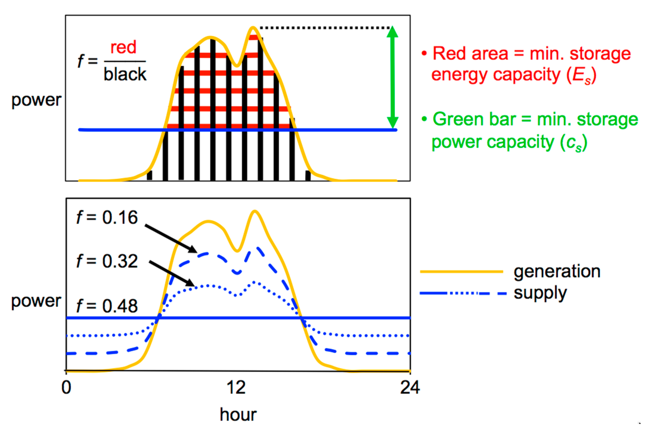
fraction of electricity generation that is stored Greater smoothing of generation peaks requires greater f (see Figure 3)
η round-trip efficiency of storage LBs usually have higher η than VFBs
e s / E s T emissions per unit of rated storage energy capacity producedg/kWhCompared to LABs, LBs generally have higher GHG emissions per rated energyTwo VFBs w/same rated energy and different rated power will have different emissions
e s / m s emissions per unit of storage mass producedg/kg
ρ specific energy capacitykWh/kg Two VFBs w/same rated energy but different power will have different ρ
D ¯ average depth of discharge (DoD) LBs are usually run at higher DoD than LABsMore “excess” storage energy capacity means lower D for same f
C cycle lifecyclesLBs have higher C than LABs
Table 2. Carbon intensities of wind generation, from wind life cycle assessment (LCA) synthesis [42,43,44,45,46,47,48,49,50,51]. Assumptions include onshore turbine size ~2 MW, offshore turbine size ~5 MW, onshore wind farm 20 km from grid with 3% transmission losses (transmission just to grid), offshore wind farm 70 km from grid with 8% transmission losses, wind farm size >50 MW, hub height 95 m, wake losses 6%, availability 97%, and offshore foundation monopile.
Carbon Intensity (gCO2e/kWh)
AvgLowHigh
Onshore high wind speed (~9 m/s)8.95.512
Onshore med wind speed (~8 m/s)9.76.412
Onshore low wind speed (~7 m/s)127.315.8
Onshore high wind speed (~9 m/s)1410.818.2

