Offshore Power Plants Integrating a Wind Farm: Design Optimisation and Techno-Economic Assessment Based on Surrogate Modelling


Abstract
:1. Introduction
2. Methods
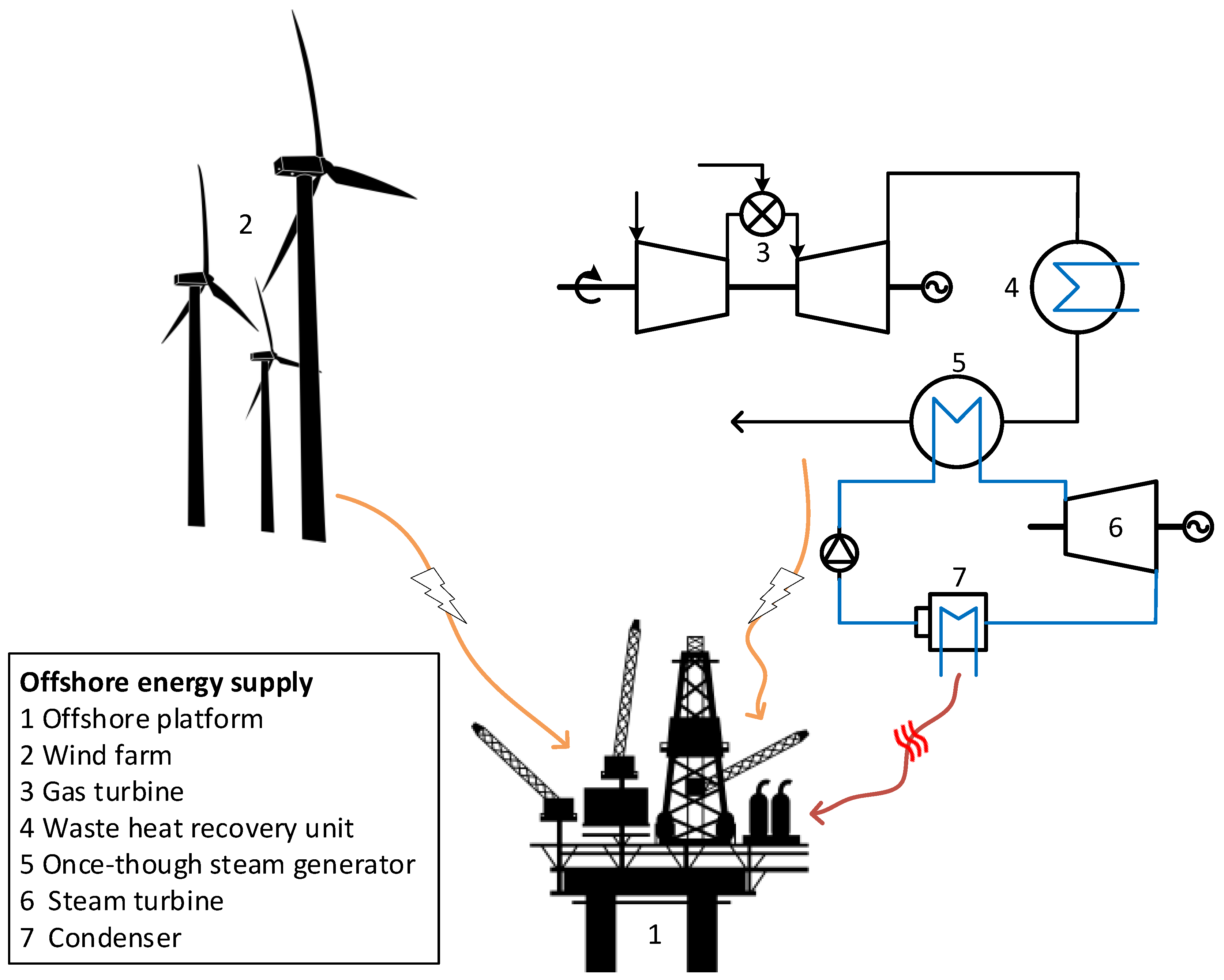
2.1. Process Modelling of the Offshore Power Plant
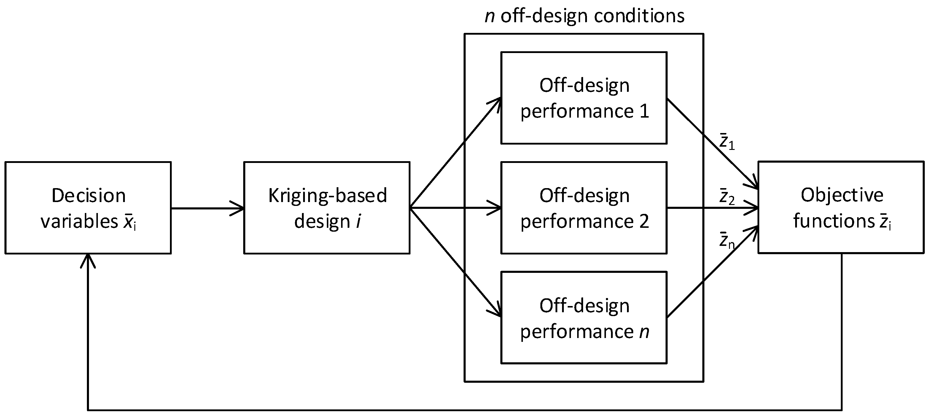
2.2. Surrogate Model Based on Kriging and Off-Design Correlation
2.3. Design Optimisation Procedure Considering Off-Design Performance
3. Case Study
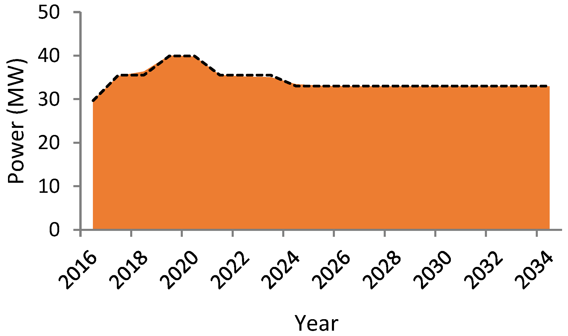
3.1. Offshore Installations
- Early life—29.7 MW (year 2016)
- Middle life—35.5 MW (years 2017 to 2018 and years 2021 to 2023)
- Peak—39.9 MW (years 2019 and 2020)
- Tail years—33.0 MW (years 2024 to 2034)
3.2. Combined Cycle
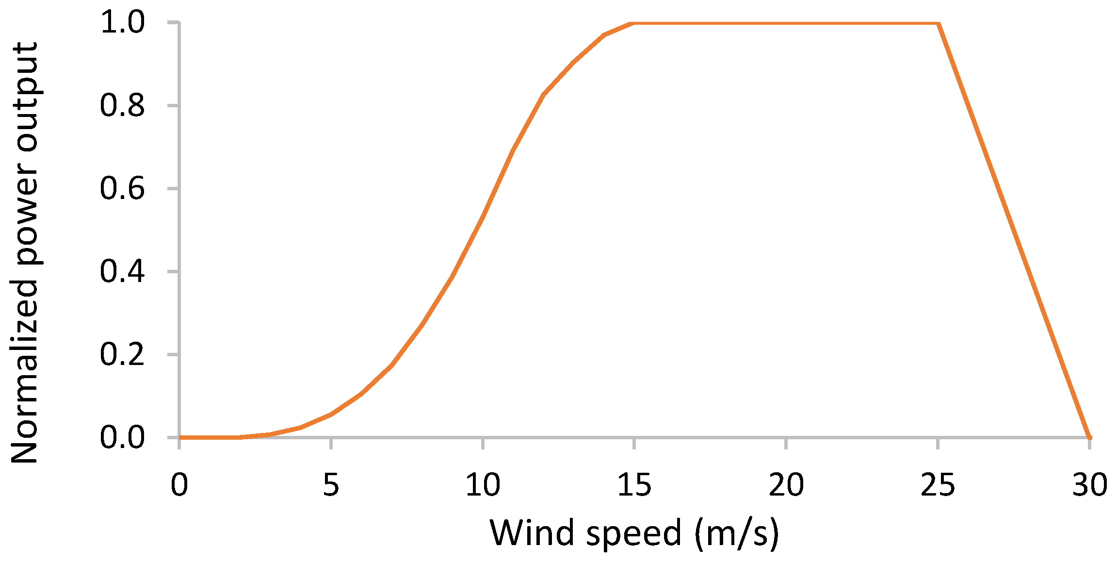
3.3. Wind Power
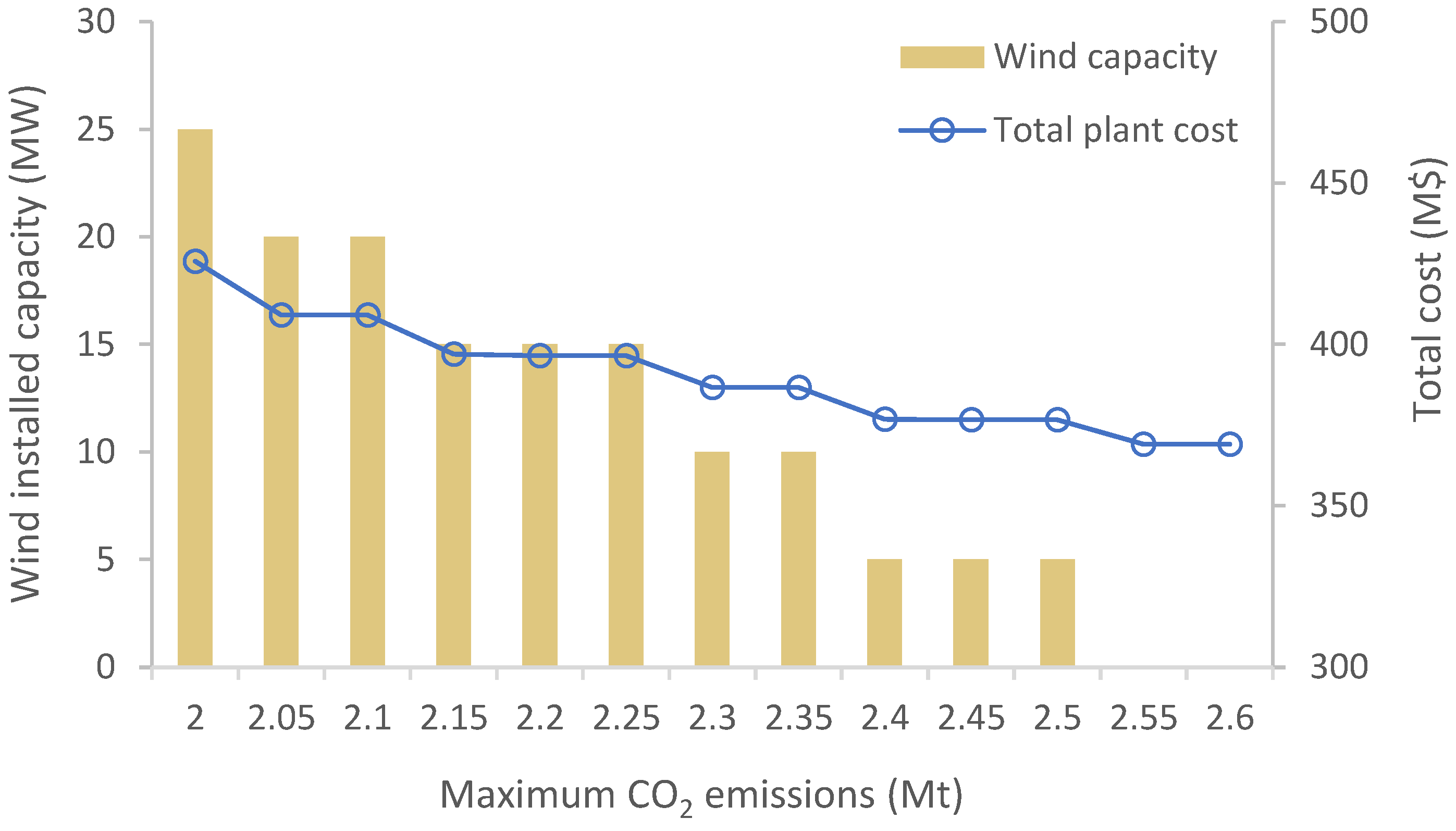
4. Results
5. Discussion and Analysis of the Results
5.1. Comparison between the Cycles Based on the Two Gas Turbines
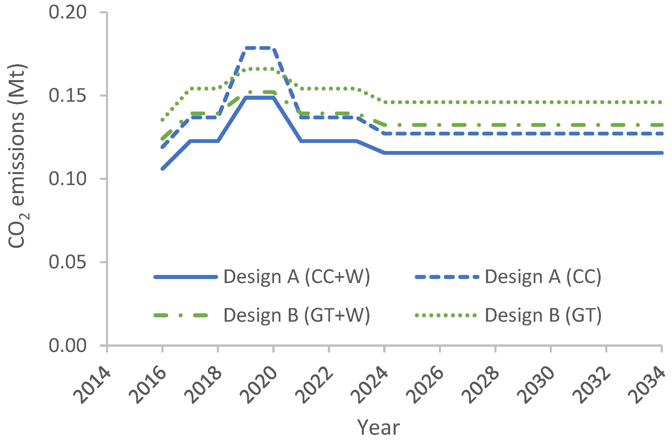
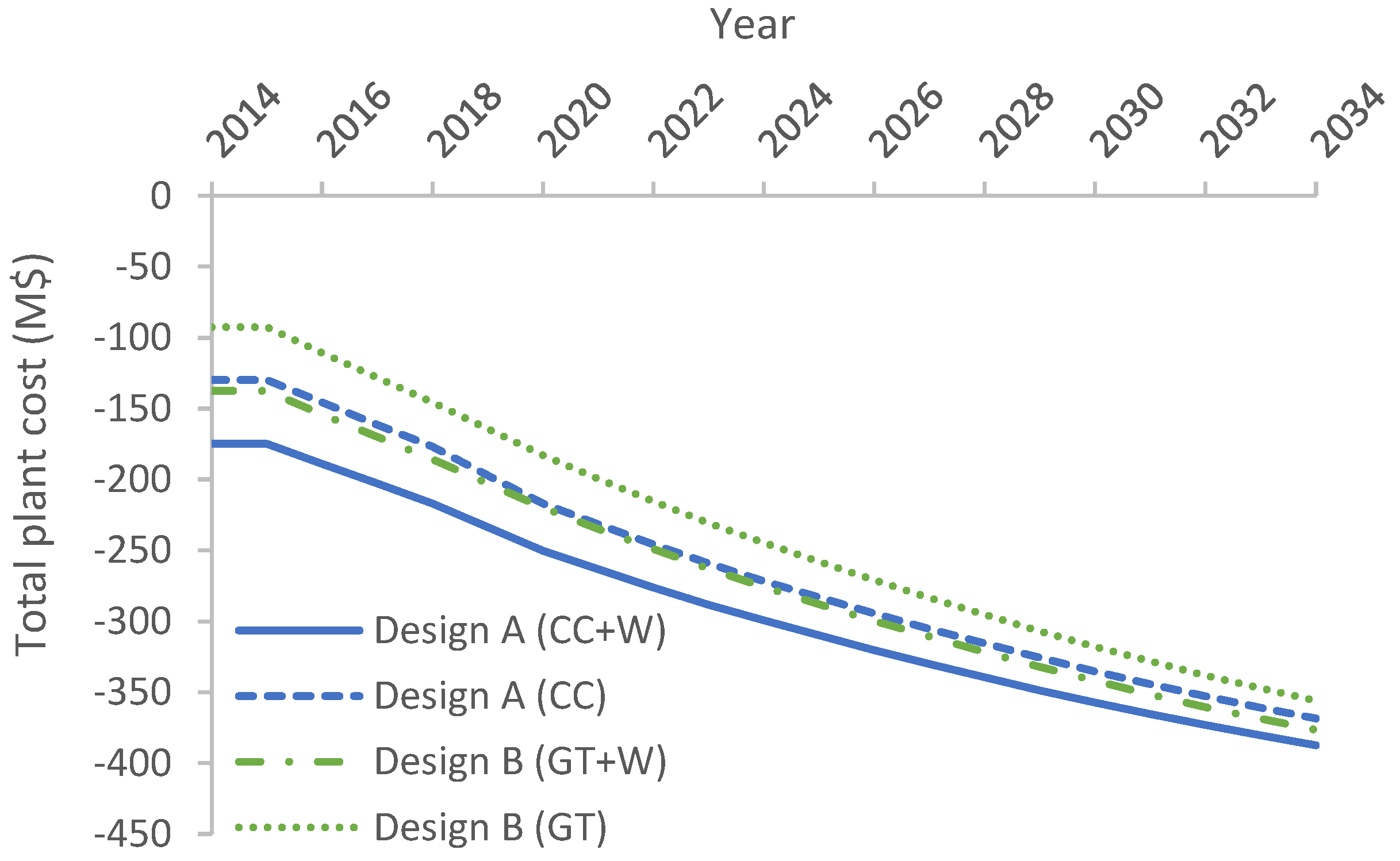
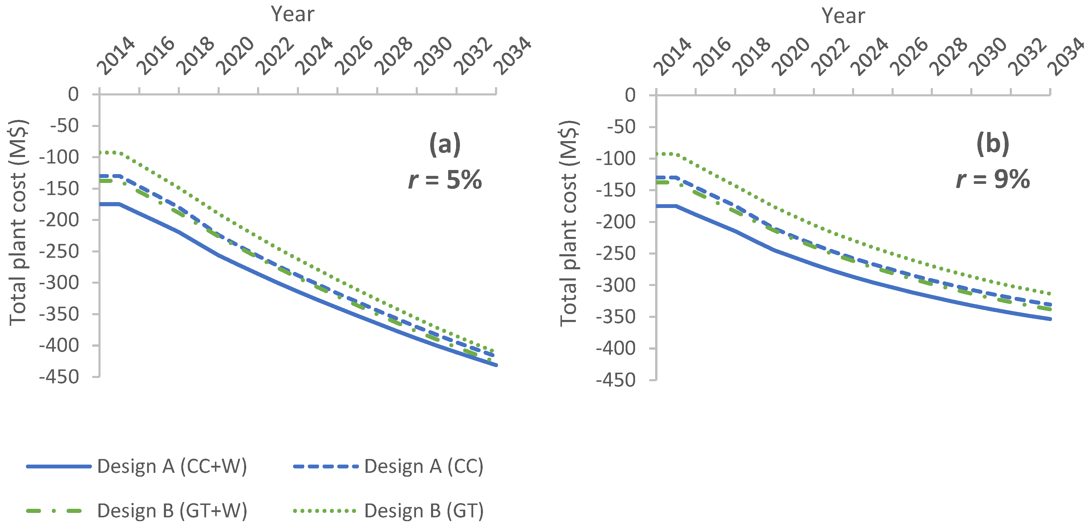
5.2. Performance Analysis of Offshore Power Plant
- Combined cycles with wind power—Design A (CC+W)
- Combined cycles—Design A (CC)
- Simple GT cycles with wind power—Design B (GT+W)
- Simple GT cycles—Design B (GT)
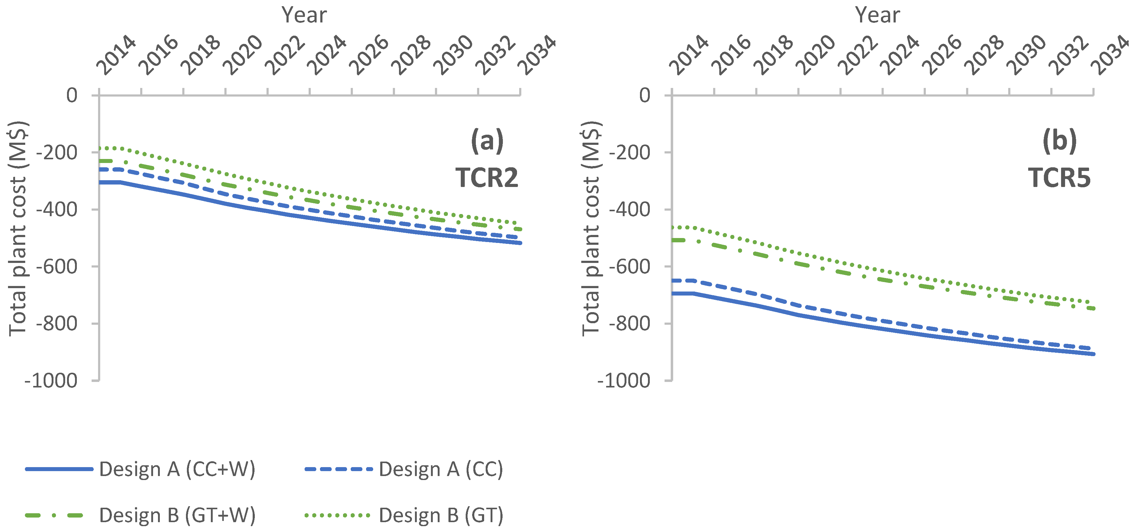
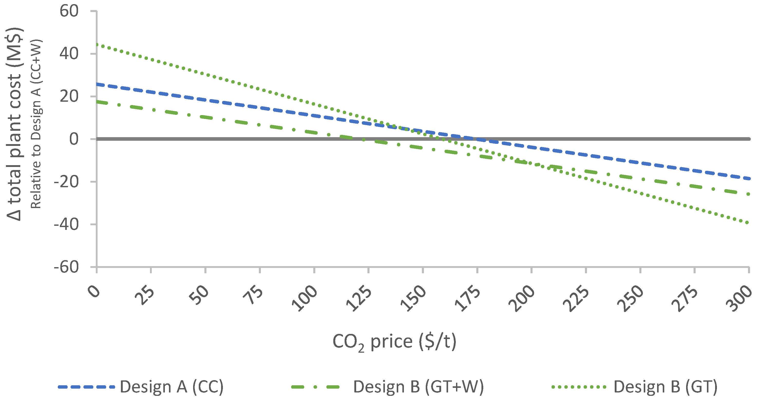
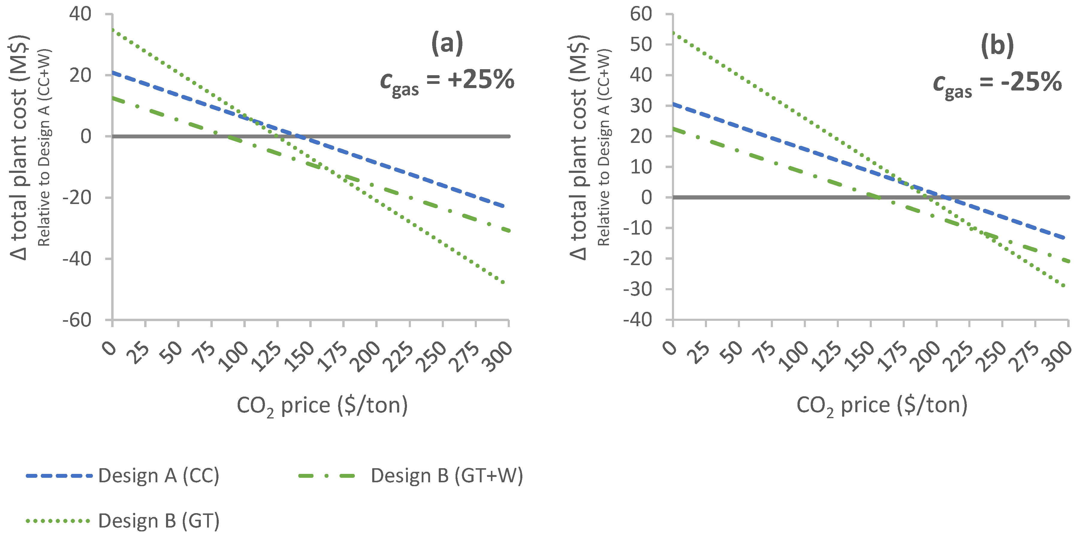
5.3. Sensitivity Analysis on Economic Parameters
6. Conclusions
Author Contributions
Funding
Conflicts of Interest
Nomenclature
| A | Heat transfer area, m2 |
| cCO2 | CO2 price, $/t |
| cgas | Gas price, $/MWh |
| CF | Cash flow |
| CFCO2 | Cash flows associated with the CO2 emissions, M$ |
| CFgas | Cash flows associated with the onsite gas consumption, M$ |
| Total CO2 emissions, Mt | |
| cost* | Total cost to supply energy to the plant, M$ |
| CS | Constant flow coefficient |
| DCF | Discounted cash flow, M$ |
| FCU | Factor accounting for copper losses |
| GT load | Gas turbine load |
| heq | Equivalent hours per year, h |
| kε | Correction factor |
| LHVgas | Lower heating value of the natural gas, kJ/kg |
| load | Mechanical load |
| ṁsteam | Steam mass flow rate, kg/s |
| mCO2 | CO2 emissions, Mt |
| ṁ | Mass flow rate, kg/s |
| ṁCO2 | Mass flow rate of emitted CO2, kg/s |
| ṁcw | Mass flow rate of cooling water, kg/s |
| ṁgas | Mass flow rate of natural gas, kg/s |
| ṁWHRU | Mass flow rate in the WHRU, kg/s |
| pcond | Condenser pressure, bar |
| pin | Turbine inlet pressure, bar |
| pout | Turbine outlet pressure, bar |
| psteam | Steam evaporation pressure, bar |
| PCC | Combined cycle power requirement, MW |
| Pnet | Net cycle power output, MW |
| PST | Steam power output, MW |
| PO | Offshore power demand, MW |
| PW | Wind power contribution, MW |
| PEC | Purchased-equipment cost, M$ |
| r | Discount rate |
| Tcond,in | Temperature at the condenser inlet, °C |
| Tin | Turbine inlet temperature, °C |
| Tsteam | Superheated steam temperature, °C |
| TCR | Total capital requirement, M$ |
| TCRCC | Total capital requirement for the combined cycle, M$ |
| TCRwind | Total capital requirement for the wind farm, M$ |
| U | Overall heat transfer coefficient, kW/K/m2 |
| UAECO1 | UA coefficient of the 1st economizer, kW/K |
| UAECO2 | UA coefficient of the 2nd economizer, kW/K |
| UAOTB | UA coefficient of the evaporator, kW/K |
| UASH | UA coefficient of the superheater, kW/K |
| UAWHRU | UA coefficient of the waste heat recovery unit, kW/K |
| Volumetric flow rate, m3/s | |
| windPW | Wind power capacity installed, MW |
| Wcomponent | Weight of the specific component of the power cycle, t |
| W* | Total weight of the bottoming cycle, t |
| WOTSG | Weight of the OTSG, t |
| WST | Weight of the steam turbine, t |
| WGEN | Weight of the generator, t |
| WCOND | Weight of the condenser (wet), t |
| Array of decision variables | |
| Array of objective functions | |
| Greek Letters | |
| γ | Exponent of the Reynolds number in the heat transfer correlation |
| Γ | Marginal likelihood |
| ΔhT,is | Isentropic enthalpy difference, kJ/kg |
| Δp | Pressure drop, bar |
| ΔpECO1 | Pressure drop in the 1st economizer, bar |
| ΔpECO2 | Pressure drop in the 2nd economizer, bar |
| ΔpOTB | Pressure drop in the evaporator, bar |
| ΔpOTSG | Overall pressure drop in the OTSG, bar |
| ΔpSH | Pressure drop in the superheater, bar |
| ΔTcw | Cooling water temperature difference, °C |
| ΔTOTSG | Pinch point difference in the OTSG, °C |
| ηcycle | Net cycle efficiency |
| ηgen | Generator efficiency |
| ηpump | Pump isentropic efficiency |
| ηT | Isentropic steam turbine efficiency |
| ϑk | Hyperparameter |
| σ2 | Process variance |
| ψ | Correlation function |
| Ψ | Correlation matrix |
| Acronyms | |
| DC | Direct costs |
| GA | Genetic algorithm |
| GT | Gas turbine |
| IC | Indirect costs |
| MAE | Mean average error |
| NOC | Number of off-design conditions |
| NPV | Net present value |
| OTSG | Once-through steam generator |
| TIT | Turbine inlet temperature |
| WHRU | Waste heat recovery unit |
Appendix A. Kriging Surrogate Modelling Technique
Appendix B. Correlations for the Off-Design Performance Predictions
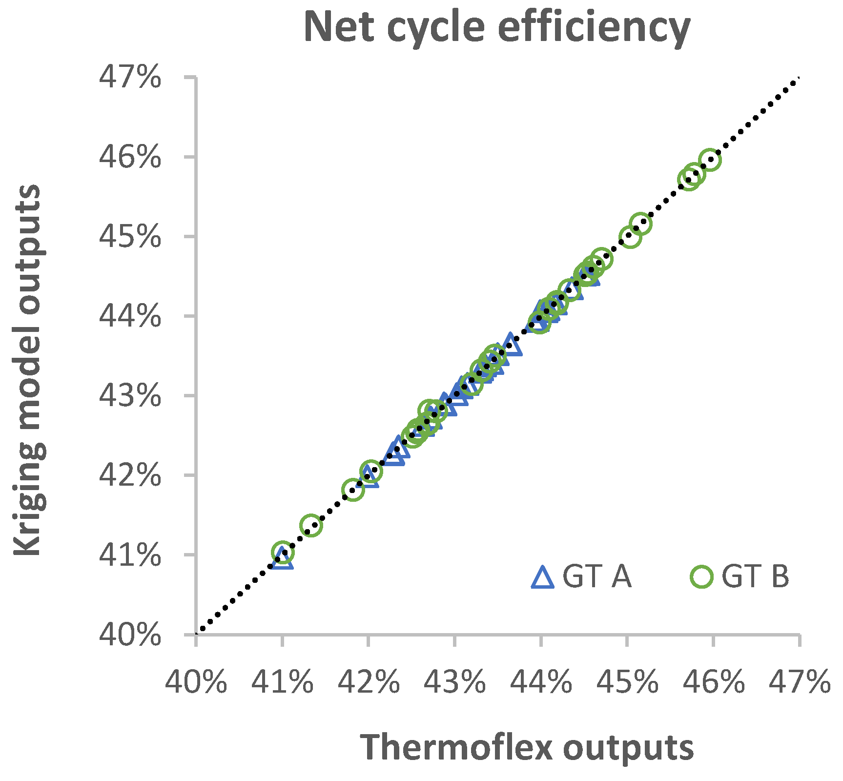
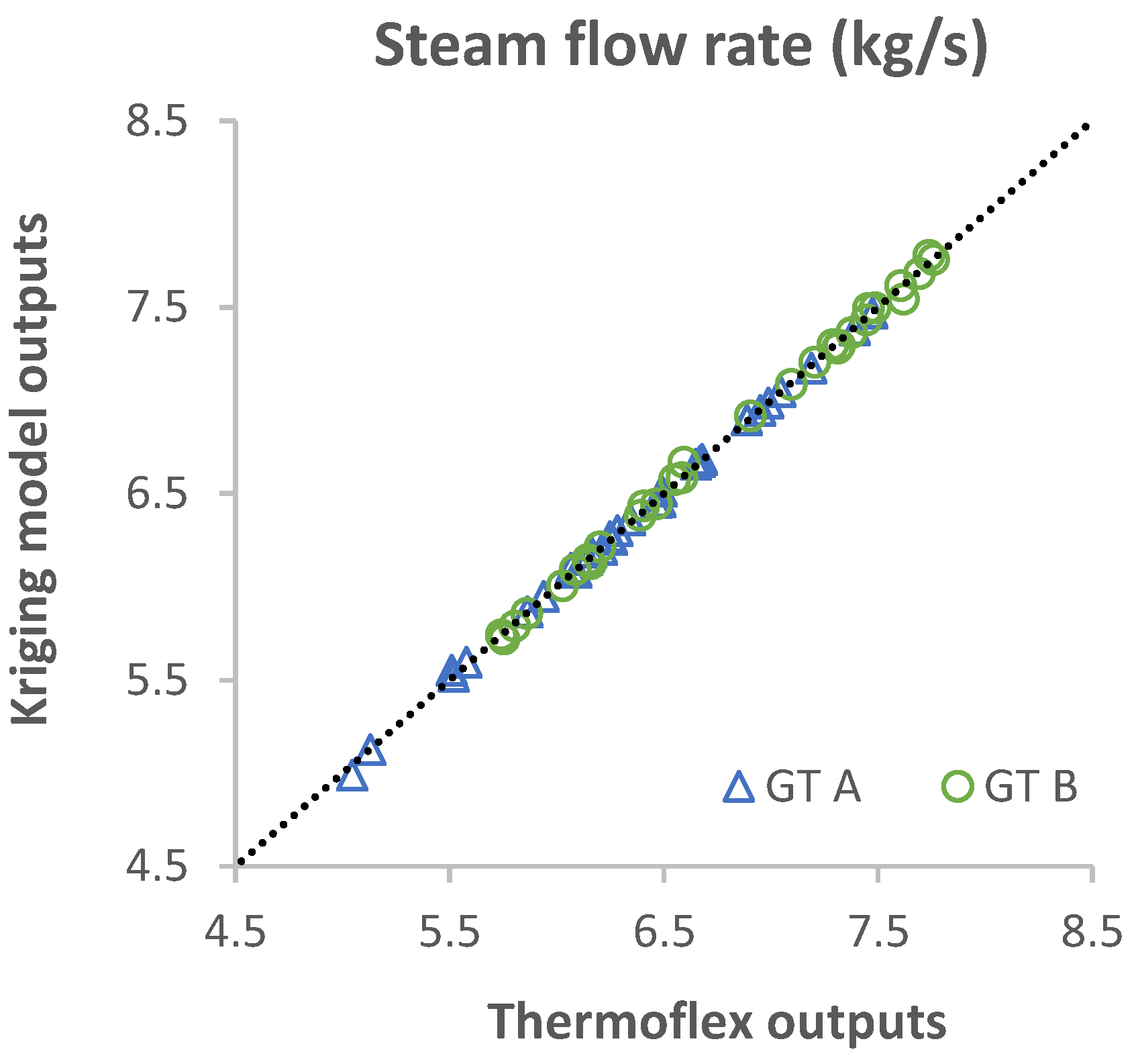
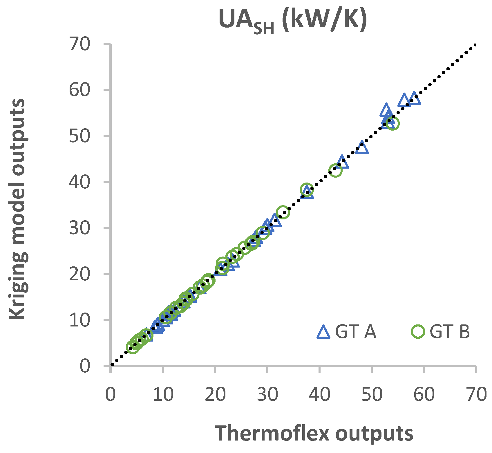
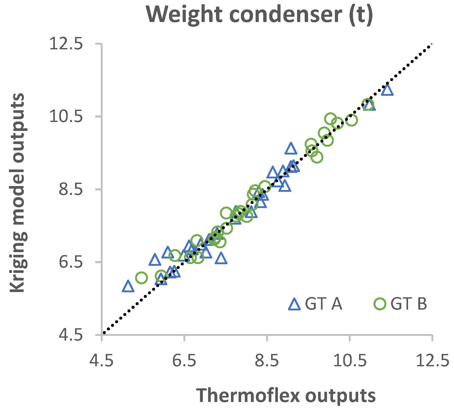
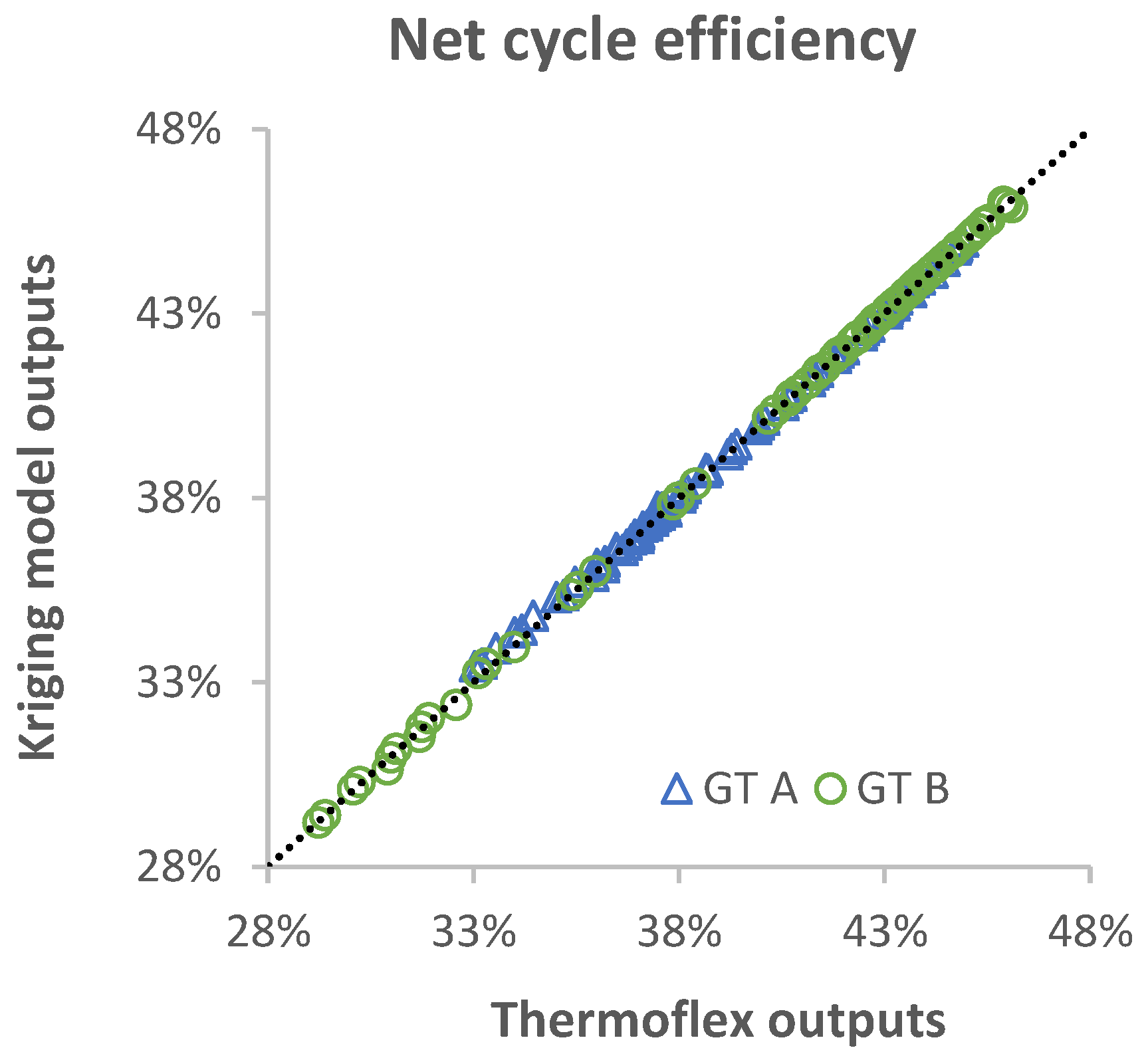
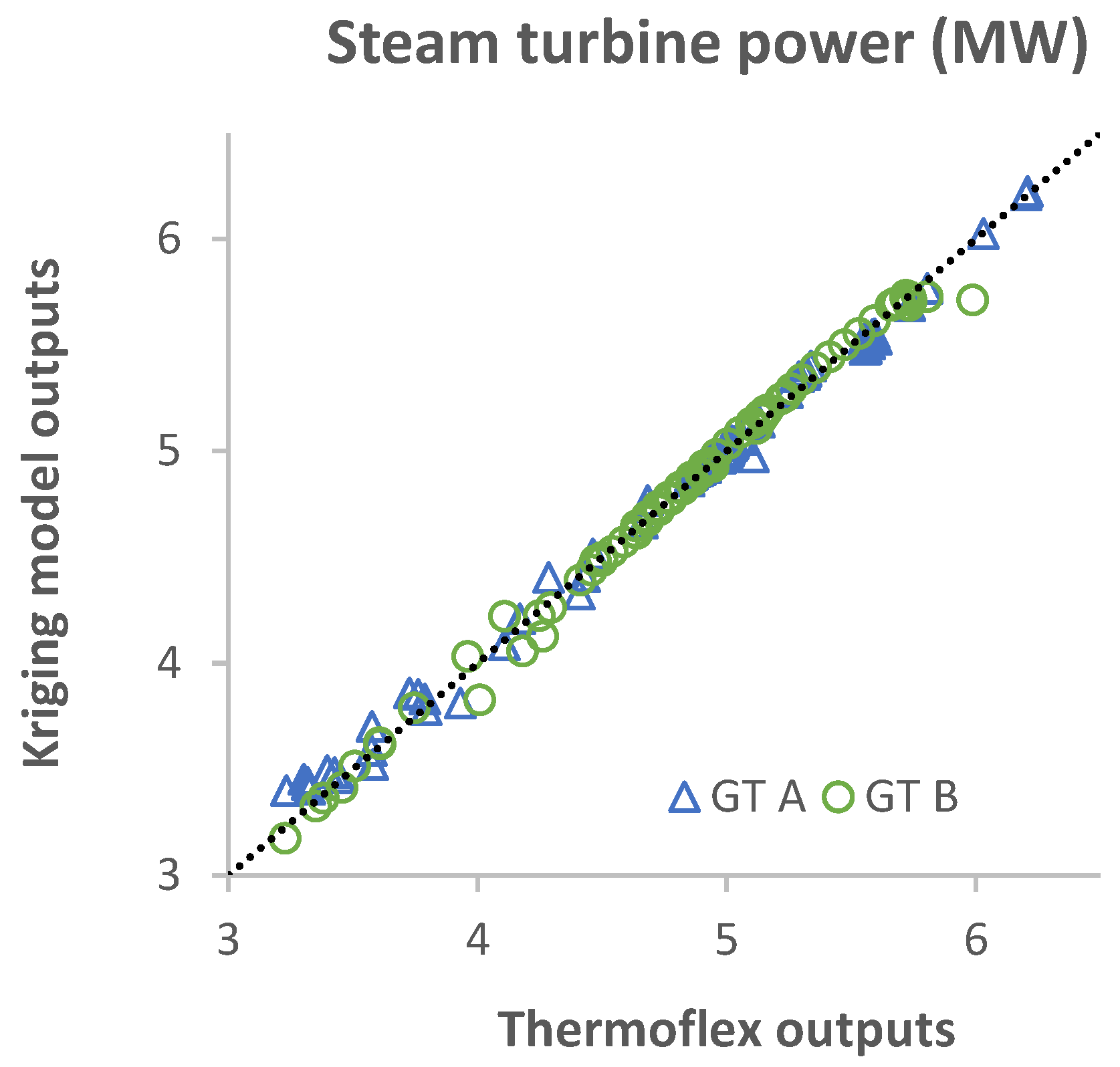
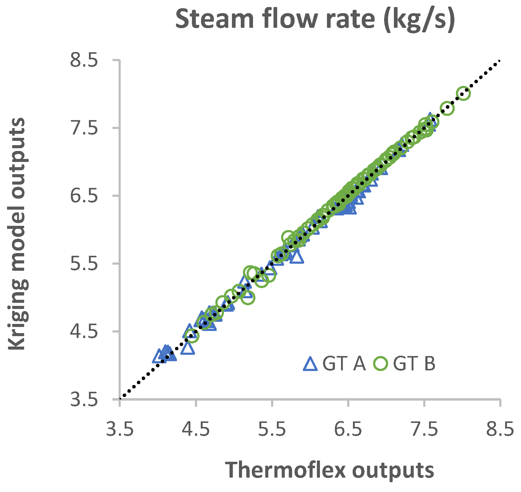
Appendix C. Validation of the Kriging Model

| Output Parameters | GT A | GT B | |
|---|---|---|---|
| Description | Symbol | MAE | MAE |
| Net cycle efficiency | ηcycle | 0.03% | 0.07% |
| Net power output | Pnet | 0.05% | 0.05% |
| Mass flow rate in the WHRU | ṁWHRU | 0.01% | 0.04% |
| UA coefficient of the WHRU | UAWHRU | 0.00% | 0.02% |
| UA coefficient of the first economizer | UAECO1 | 0.58% | 0.78% |
| UA coefficient of the second economizer | UAECO2 | 0.52% | 0.68% |
| UA coefficient of the evaporator | UAOTB | 0.30% | 0.44% |
| UA coefficient of the superheater | UASH | 1.35% | 1.28% |
| Pressure drop in the first economizer | ΔpECO1 | 0.00% | 0.00% |
| Pressure drop in the second economizer | ΔpECO2 | 0.03% | 0.04% |
| Pressure drop in the evaporator | ΔpOTB | 1.02% | 0.99% |
| Pressure drop in the superheater | ΔpSH | 0.00% | 0.00% |
| Steam mass flow rate | ṁsteam | 0.23% | 0.29% |
| Isentropic steam turbine efficiency | ηT | 0.39% | 0.43% |
| Temperature at the condenser inlet | Tcond,in | 0.00% | 0.00% |
| Mass flow rate of cooling water | ṁcw | 0.54% | 0.56% |
| Weight of the OTSG | WOTSG | 0.42% | 0.56% |
| Weight of steam turbine | WST | 0.48% | 0.41% |
| Weight of generator | WGEN | 0.19% | 0.27% |
| Weight of the condenser (wet) | WCOND | 3.18% | 2.30% |
| Purchased-equipment cost | PEC | 0.23% | 0.27% |


Appendix D. Validation of the Off-Design Correlations
| GT A | GT B | |||||
|---|---|---|---|---|---|---|
| Design #1 | Design #2 | Design #3 | Design #1 | Design #2 | Design #3 | |
| GT load | 0.90 | 0.82 | 0.93 | 0.90 | 0.69 | 0.82 |
| psteam | 20 | 32 | 27 | 30 | 18 | 35 |
| Tsteam | 328 | 390 | 360 | 350 | 320 | 290 |
| ΔTOTSG | 25 | 20 | 15 | 25 | 12 | 18 |
| pcond | 0.07 | 0.05 | 0.04 | 0.07 | 0.04 | 0.09 |
| ΔTcw | 8 | 5 | 6 | 8 | 5 | 4 |
| Design #1 | Design #2 | Design #3 | Overall | |
|---|---|---|---|---|
| MAE | MAE | MAE | MAE | |
| GT A | ||||
| ηcycle | 0.20% | 0.26% | 0.27% | 0.24% |
| Pnet | 0.20% | 0.26% | 0.27% | 0.24% |
| ṁCO2 | 0.00% | 0.00% | 0.00% | 0.00% |
| PST | 0.87% | 1.18% | 1.21% | 1.08% |
| psteam | 0.79% | 1.13% | 1.26% | 1.06% |
| Tsteam | 0.45% | 0.21% | 0.29% | 0.32% |
| ṁsteam | 0.66% | 0.79% | 1.06% | 0.84% |
| GT B | ||||
| ηcycle | 0.12% | 0.17% | 0.05% | 0.11% |
| Pnet | 0.12% | 0.17% | 0.05% | 0.12% |
| ṁCO2 | 0.00% | 0.00% | 0.01% | 0.01% |
| PST | 0.57% | 1.00% | 0.42% | 0.66% |
| psteam | 0.80% | 1.19% | 0.50% | 0.83% |
| Tsteam | 0.41% | 0.12% | 0.63% | 0.39% |
| ṁsteam | 0.67% | 0.69% | 0.52% | 0.63% |


References
- Nguyen, T.-V.; Tock, L.; Breuhaus, P.; Maréchal, F.; Elmegaard, B. CO2-mitigation options for the offshore oil and gas sector. Appl. Energy 2016, 161, 673–694. [Google Scholar] [CrossRef] [Green Version]
- Statistisk Sentralbyrå. Utslipp av klimagasser 2015; Statistisk Sentralbyrå: Oslo, Norway, 2016. [Google Scholar]
- Riboldi, L.; Nord, L.O. Concepts for lifetime efficient supply of power and heat to offshore installations in the North Sea. Energy Convers. Manag. 2017, 148, 860–875. [Google Scholar] [CrossRef]
- Nguyen, T.-V.; Voldsund, M.; Breuhaus, P.; Elmegaard, B. Energy efficiency measures for offshore oil and gas platforms. Energy 2016, 117, 1–16. [Google Scholar] [CrossRef]
- Pierobon, L.; Benato, A.; Scolari, E.; Haglind, F.; Stoppato, A. Waste heat recovery technologies for offshore platforms. Appl. Energy 2014, 136, 228–241. [Google Scholar] [CrossRef] [Green Version]
- Mazzetti, J.M.; Nekså, P.; Walnum, H.T.; Hemmingsen, A.K.T. Energy-Efficient Technologies for Reduction of Offshore CO2 Emmissions. In Proceedings of the Offshore Technology Conference, Houston, TX, USA, 6–9 May 2013. [Google Scholar]
- Nord, L.O.; Bolland, O. Design and off-design simulations of combined cycles for offshore oil and gas installations. Appl. Therm. Eng. 2013, 54, 85–91. [Google Scholar] [CrossRef] [Green Version]
- Nord, L.O.; Martelli, E.; Bolland, O. Weight and power optimization of steam bottoming cycle for offshore oil and gas installations. Energy 2014, 76, 891–898. [Google Scholar] [CrossRef] [Green Version]
- Pierobon, L.; Van Nguyen, T.; Larsen, U.; Haglind, F.; Elmegaard, B. Multi-objective optimization of organic Rankine cycles for waste heat recovery: Application in an offshore platform. Energy 2013, 58, 538–549. [Google Scholar] [CrossRef] [Green Version]
- Riboldi, L.; Nord, L.O. Lifetime assessment of combined cycles for cogeneration of power and heat in offshore oil and gas installations. Energies 2017, 10, 744. [Google Scholar] [CrossRef]
- Econ Pöyry. CO2-Emissions Effect of Electrification; Econ Pöyry: Helsinki, Finland, 2011. [Google Scholar]
- Riboldi, L.; Cheng, X.; Farahmand, H.; Korpås, M.; Nord, L.O. Effective concepts for supplying energy to a large offshore oil and gas area under different future scenarios. Chem. Eng. Trans. 2017, 61, 1597–1602. [Google Scholar]
- He, W.; Jacobsen, G.; Anderson, T.; Olsen, F.; Hanson, T.D.; Korpås, M.; Toftevaag, T.; Eek, J.; Uhlen, K.; Johansson, E. The potential of integrating wind power with offshore oil and gas platforms. Wind Eng. 2010, 34, 125–137. [Google Scholar] [CrossRef]
- Elginoz, N.; Bas, B. Life Cycle Assessment of a multi-use offshore platform: Combining wind and wave energy production. Ocean Eng. 2017, 145, 430–443. [Google Scholar] [CrossRef]
- Korpås, M.; Warland, L.; He, W.; Tande, J.O.G. A case-study on offshore wind power supply to oil and gas rigs. Energy Procedia 2012, 24, 18–26. [Google Scholar] [CrossRef]
- Bianchi, M.; Branchini, L.; De Pascale, A.; Melino, F.; Orlandini, V.; Peretto, A.; Haglind, F.; Pierobon, L. Cogenerative performance of a wind-gas turbine-organic rankine cycle integrated system for offshore applications. In Proceedings of the ASME Turbo Expo 2016, Seoul, Korea, 13–17 June 2016; Volume 3. [Google Scholar]
- Orlandini, V.; Pierobon, L.; Schløer, S.; De Pascale, A.; Haglind, F. Dynamic performance of a novel offshore power system integrated with a wind farm. Energy 2016, 109, 236–247. [Google Scholar] [CrossRef] [Green Version]
- Riboldi, L.; Nord, L.O. Optimal design of flexible power cycles through Kriging-based surrogate models. In Proceedings of the ASME Turbo Expo 2018: Turbomachinery Technical Conference and Exposition, Oslo, Norway, 11–15 June 2018. [Google Scholar]
- Kang, C.A.; Brandt, A.R.; Durlofsky, L.J. Optimal operation of an integrated energy system including fossil fuel power generation, CO2 capture and wind. Energy 2011, 36, 6806–6820. [Google Scholar] [CrossRef]
- Kang, C.A.; Brandt, A.R.; Durlofsky, L.J. A new carbon capture proxy model for optimizing the design and time-varying operation of a coal-natural gas power station. Int. J. Greenh. Gas Control 2016, 48, 234–252. [Google Scholar] [CrossRef]
- Thermoflex, Version 26.0; Thermoflow Inc.: Fayville, MA, USA, 2016.
- Nord, L.O.; Bolland, O. Steam bottoming cycles offshore—Challenges and possibilities. J. Power Technol. 2012, 92, 201–207. [Google Scholar]
- Kehlhofer, R. Combined-Cycle Gas & Steam Turbine Power Plants; Pennwell Books: Houston, TX, USA, 1999. [Google Scholar]
- Couckuyt, I.; Dhaene, T.; Demeester, P. ooDACE toolbox: A flexible object-oriented kriging implementation. J. Mach. Learn. Res. 2014, 15, 3183–3186. [Google Scholar]
- Incropera, F.P.; DeWitt, D.P.; Bergman, T.L.; Lavine, A.S. Fundamentals of Heat and Mass Transfer; John Wiley & Sons: Hoboken, NJ, USA, 2007; Volume 6. [Google Scholar]
- Haglind, F. Variable geometry gas turbines for improving the part-load performance of marine combined cycles - Combined cycle performance. Appl. Therm. Eng. 2011, 31, 467–476. [Google Scholar] [CrossRef]
- Schobeiri, M. Turbomachinery Flow Physics and Dynamic Performance; Springer: Berlin, Germany, 2005. [Google Scholar]
- Haglind, F.; Elmegaard, B. Methodologies for predicting the part-load performance of aero-derivative gas turbines. Energy 2009, 34, 1484–1492. [Google Scholar] [CrossRef]
- Veres, J.P. Centrifugal and Axial Pump Design and Off-Design Performance Prediction; NASA Techincal Memo 106745; NASA Lewis Research Center: Cleveland, OH, USA, 1995; pp. 1–24.
- Bejan, A.; Tsatsaronis, G.; Moran, M. Thermal Design and Optimization; John Wiley & Sons: Hoboken, NJ, USA, 1996. [Google Scholar]
- Carlsson, J.; Fortes, M.D.; de Marco, G.; Giuntoli, J.; Jakubcionis, M.; Jäger-Waldau, A.; Lacal-Arantegui, R.; Lazarou, S.; Magagna, D.; Moles, C.; et al. ETRI 2014—Energy Technology Reference Indicator projections for 2010–2050; JRC Sci Policy Reports; European Commission: Brussels, Belgium, 2014; pp. 1–108. [Google Scholar]
- International Energy Agency (IEA). World Energy Outlook 2016; International Energy Agency: Paris, France, 2016; pp. 1–684. [Google Scholar]
- Directorate, Norwegian Petroleum. Ministry of Petroleum and Energy; Norwegian Petroleum: Stavanger, Norway, 2017.
- MathWorks. Global Optimization Toolbox, Version R2015a; MathWorks: Natick, MA, USA, 2016. [Google Scholar]
- Lundin; Wintershall; RWE. Plan for Utbygging, Anlegg og Drift av Luno—Del 2: Konsekvensutredning. 2011. Available online: https://www.lundin-petroleum.com/Documents/ot_no_Luno_EIA_2011.pdf (accessed on 15 October 2018).
- Det Norske Oljeselskap ASA. Plan for Utbygging og Drift av Ivar Aasen—Del 2: Konsekvensutredning. 2012. Available online: https://docplayer.me/423297-Plan-for-utbygging-og-drift-av-ivar-aasen.html (accessed on 15 October 2018).
- Berge, E.; Byrkjedal, Ø.; Ydersbond, Y.; Kindler, D. Modelling of offshore wind resources. Comparison of a meso-scale model and measurements from FINO 1 and North Sea oil rigs. Eur. Wind Energy Conf. Exhib. 2009, 4, 2327–2334. [Google Scholar]
- StatoilHydro. The World’s Firs Full Scale Floating Wind Turbine; Hywind by StatoilHydro: Stavanger, Norway, 2009. [Google Scholar]
- Rúa, J.; Montañés, R.M.; Riboldi, L.; Nord, L.O. Dynamic Modeling and Simulation of an Offshore Combined Heat and Power (CHP) Plant. In Proceedings of the 58th Conference on Simulation and Modelling (SIMS 58), Reykjavik, Iceland, 25–27 September 2017; Linköping University Electronic Press: Linköping, Sweden, 2017; pp. 241–250. [Google Scholar]
- Nord, L.O.; Montañés, R.M. Compact steam bottoming cycles: Model validation with plant data and evaluation of control strategies for fast load changes. Appl. Therm. Eng. 2018, 142, 334–345. [Google Scholar] [CrossRef]
- Sacks, J.; Welch, W.J.; Mitchell, T.J.; Wynn, H.P. Design and analysis of computer experiments. Stat. Sci. 1989, 4, 409–423. [Google Scholar] [CrossRef]
- Koziel, S.; Yang, X. Computational Optimization, Methods and Algorithms; Springer: Berlin, Germany, 2011. [Google Scholar]
- Jones, D.R.; Schonlau, M.; Welch, W.J. Efficient global optimization of expensive black-box functions. J. Glob. Optim. 1998, 13, 455–492. [Google Scholar] [CrossRef]
- Simpson, T.W.; Peplinski, J.D.; Koch, P.N.; Allen, J.K. Metamodels for computer-based engineering design: Survey and recommendations. Eng. Comput. 2001, 17, 129–150. [Google Scholar] [CrossRef]
- Cooke, D.H. On prediction of off-design multistage turbine pressures by stodola’s ellipse. J. Eng. Gas Turbines Power 1985, 107, 596–606. [Google Scholar] [CrossRef]
- Lecompte, S.; Huisseune, H.; van den Broek, M.; De Schampheleire, S.; De Paepe, M. Part load based thermo-economic optimization of the Organic Rankine Cycle (ORC) applied to a combined heat and power (CHP) system. Appl. Energy 2013, 111, 871–881. [Google Scholar] [CrossRef]


| Direct Cost (DC) | Range from [30] | Factor Selected |
|---|---|---|
| Onsite cost | ||
| Purchased-equipment costs (PEC) | ||
| Purchased-equipment installation | 20–90% of PEC | 45% |
| Piping | 10–70% of PEC | 35% |
| Instrumentation and controls | 6–40% of PEC | 20% |
| Electrical equipment and materials | 10–15% of PEC | 11% |
| Offsite cost | ||
| Civil, structural and architectural work | 15–90% of PEC | 30% |
| Service facilities | 30–100% of PEC | 65% |
| Indirect Cost (IC) | ||
| Engineering and supervision | 6–15% of DC | 8% |
| Construction costs and constructors profit | 15% of DC | 15% |
| Contingencies | 8–25% of total cost | 25% |
| Input Parameters | GT A | GT B | |||
|---|---|---|---|---|---|
| Description | Symbol | Lower Bound | Upper Bound | Lower Bound | Upper Bound |
| Gas turbine load | GT load | 0.80 | 0.95 | 0.60 | 0.95 |
| Steam evaporation pressure (bar) | psteam | 15 | 40 | 15 | 40 |
| Superheated steam temperature (°C) | Tsteam | 300 | 410 | 280 | 370 |
| Pinch point temperature difference in the OTSG (°C) | ΔTOTSG | 10 | 30 | 10 | 30 |
| Condenser pressure (bar) | pcond | 0.03 | 0.10 | 0.03 | 0.12 |
| Condenser cooling water temperature difference (°C) | ΔTcw | 3 | 10 | 3 | 10 |
| Power Demand Offshore | Wind Power | Combined Cycle Power |
|---|---|---|
| PO | PW | PCC = PO − PW |
| MW | MW | MW |
| 29.7 (year 2016) | 10.0 | 19.7 |
| 7.5 | 22.2 | |
| 5.0 | 24.7 | |
| 2.5 | 27.2 | |
| 0.0 | 29.7 | |
| 35.5 (years 2017 to 2018 and years 2021 to 2023) | 10.0 | 25.5 |
| 7.5 | 28.0 | |
| 5.0 | 30.5 | |
| 2.5 | 33.0 | |
| 0.0 | 35.5 | |
| 39.9 (years 2019 and 2020) | 10.0 | 29.9 |
| 7.5 | 32.4 | |
| 5.0 | 34.9 | |
| 2.5 | 37.4 | |
| 0.0 | 39.9 | |
| 33.0 (years 2024 and 2034) | 10.0 | 23.0 |
| 7.5 | 25.5 | |
| 5.0 | 28.0 | |
| 2.5 | 30.5 | |
| 0.0 | 33.0 |
| GT A | ||||
|---|---|---|---|---|
| Design A (CC+W) | Design A (CC) | Design A (GT+W) | Design A (GT) | |
| Decision variables | ||||
| GT load | 0.86 | 0.86 | - | - |
| psteam (bar) | 17.7 | 17.7 | - | - |
| Tsteam (°C) | 355.8 | 355.8 | - | - |
| ΔTOTSG (°C) | 18.3 | 18.3 | - | - |
| pcond (bar) | 0.09 | 0.09 | - | - |
| ΔTcw (°C) | 6.1 | 6.1 | - | - |
| windPW (MW) | 10 | - | 10 | - |
| Objective functions | ||||
| (Mt) | 2.3 | 2.6 | 2.8 | 3.3 |
| W* (t) | 102 | 102 | - | - |
| cost* (M$) | 387 | 369 | 396 | 399 |
| GT B | ||||
|---|---|---|---|---|
| Design B (CC+W) | Design B (CC) | Design B (GT+W) | Design B (GT) | |
| Decision variables | ||||
| GT load | 0.62 | 0.62 | - | - |
| psteam (bar) | 16.7 | 16.7 | - | - |
| Tsteam (°C) | 323.3 | 323.3 | - | - |
| ΔTOTSG (°C) | 24.7 | 24.7 | - | - |
| pcond (bar) | 0.09 | 0.09 | - | - |
| ΔTcw (°C) | 5.8 | 5.8 | - | - |
| windPW (MW) | 15 | - | 10 | - |
| Objective functions | ||||
| (Mt) | 2.3 | 2.6 | 2.6 | 2.8 |
| W* (t) | 104 | 104 | - | - |
| cost* (M$) | 407 | 369 | 377 | 356 |
© 2018 by the authors. Licensee MDPI, Basel, Switzerland. This article is an open access article distributed under the terms and conditions of the Creative Commons Attribution (CC BY) license (http://creativecommons.org/licenses/by/4.0/).
Share and Cite
Riboldi, L.; Nord, L.O. Offshore Power Plants Integrating a Wind Farm: Design Optimisation and Techno-Economic Assessment Based on Surrogate Modelling. Processes 2018, 6, 249. https://doi.org/10.3390/pr6120249
Riboldi L, Nord LO. Offshore Power Plants Integrating a Wind Farm: Design Optimisation and Techno-Economic Assessment Based on Surrogate Modelling. Processes. 2018; 6(12):249. https://doi.org/10.3390/pr6120249
Chicago/Turabian StyleRiboldi, Luca, and Lars O. Nord. 2018. "Offshore Power Plants Integrating a Wind Farm: Design Optimisation and Techno-Economic Assessment Based on Surrogate Modelling" Processes 6, no. 12: 249. https://doi.org/10.3390/pr6120249