Low-Carbon-Oriented Capacity Optimization Method for Electric–Thermal Integrated Energy System Considering Construction Time Sequence and Uncertainty

Abstract

The interdependence of various energy forms and flexible cooperative operation between different units in an integrated energy system (IES) are essential for carbon emission reduction. To address the planning problem of an electric–thermal integrated energy system under low-carbon conditions and to fully consider the low carbon and construction sequence of the integrated energy system, a low-carbon-oriented capacity optimization method for the electric–thermal integrated energy system that considers construction time sequence (CTS) and uncertainty is proposed. A calculation model for the carbon transaction cost under the ladder carbon trading mechanism was constructed, and a multi-stage planning model of the integrated energy system was established with the minimum life cycle cost, considering carbon transaction cost as the objective function, to make the optimal decision on equipment configuration in each planning stage. Finally, a case study was considered to verify the advantages of the proposed capacity optimization method in terms of economy and environmental friendliness through a comparative analysis of different planning cases. Simulation results show that, compared with the scenario of completing planning at the beginning of the life cycle at one time, the proposed low-carbon-oriented capacity optimization method that considers construction time sequence and uncertainty can not only reduce the cost of the integrated energy system, but also help to enhance renewable energy utilization and reduce the system’s carbon emissions; the total cost of phased planning is reduced by 11.91% compared to the total cost of one-time planning at the beginning of the year.

1. Introduction

Under the background of increasingly severe global environmental problems, carbon emission reduction has become a priority of all countries. At the 75th United Nations General Assembly, China announced that it will increase its nationally determined carbon contributions, reach peak carbon emissions by 2030, and strive to achieve carbon neutrality by 2060 [1]. New rules on carbon emissions pose more stringent requirements for the future development of energy systems in China. With the increasing energy demand and environmental pressure, the integrated energy system (IES) is an essential technology required to improve energy efficiency and reduce carbon emissions [2]. However, the energy types and energy conversion equipment in the IES are diverse and complex. To fully realize a capacity for carbon emission reduction, carbon emission factors should be considered in the planning stage of IESs.

Under the current development status of carbon emission reduction technology, carbon capture and conversion technology and renewable energy power generation are the principal means for an IES to reduce carbon emissions. At present, the power-to-gas (P2G) technology and carbon capture technology have been widely used in IESs. A P2G system can absorb carbon dioxide to synthesize methane and convert electricity into gas, which is of great significance in promoting the low-carbon development of IESs [3]. Zhang et al. [4] proposed an optimized design method for a residential IES employing the P2G technology with multi-functional characteristics. Li et al. [5] studied multi-objective optimization and agent-based modeling for a 100% renewable island IES considering P2G technology and extreme weather conditions. Liu et al. [6] studied the planning method of an integrated energy system based on two-stage robust optimization and the non-cooperative game method. Zhang et al. [7] established a day-ahead optimal dispatching method that employs P2G units and dynamic pipeline networks. Cui et al. [8] developed a low-carbon and economic scheduling framework that integrates the operation of carbon capture power plants, P2G units, and the price-based demand response. The power-to-hydrogen model and seasonal hydrogen storage model were proposed in [9] to deal with the optimal planning of an IES. Guo et al. [10] studied the low-carbon operation method of integrated plants based on carbon capture units. Guo et al. [11] proposed a low-carbon planning method for an integrated energy station considering combined P2G and gas-fired units equipped with carbon capture systems.

In addition to employing P2G and carbon capture systems, increasing the capacity of renewable energy in IESs is also an important means of carbon emission reduction. To ensure the reliable and efficient operation of IESs, the uncertainty and volatility of renewable energy are the problems that must be solved in the planning and operation of IESs. He et al. [12] presented a distributed, robust planning methodology that incorporates the electric–thermal demand response and the inertia of thermal loads. Cao et al. [13] proposed a two-stage robust stochastic programming model for energy hub capacity planning with a distributional robustness guarantee. Ozy et al. [14] proposed an adaptive, robust planning method for distribution systems that considers the siting and sizing of renewable energy structures. Pan et al. [15] proposed a decentralized robust planning method for a multi-stakeholder IES under source–load uncertainties. Ge et al. [16] presented an optimal planning model for an IES that considers distributed generation uncertainties and carbon emission punishments. Li et al. [17] proposed an energy hub-based optimal planning framework for a user-level IES that considers synergistic effects under multiple uncertainties. Lei et al. [18] proposed a multi-stage scenario tree generation method for a long time scale with multiple uncertainties based on a Markov chain.

In addition, the strict carbon emission reduction market policy urges IESs to have their carbon emission reduction capabilities enhanced. Building the National Carbon Emission Trading Market (NCET) is one of the planned means for China to achieve its goals of carbon peak and carbon neutrality. The NCET was piloted in seven cities in 2017, and the first batch of crucial emission units incorporated into the market covers almost 1700 thermal power generation enterprises in China [19]. In 2021, the launching ceremony of the NCET was held in Beijing, Shanghai, and Wuhan, simultaneously, and the high-profile NCET officially began online trading. According to the transaction rules of the NCET, an IES can enjoy a carbon quota that matches its power generation capacity. The IES can independently optimize the operation strategy of the system, and the surplus or insufficient carbon quota of the IES can be traded through the NCET. Driven by the strict policy, some studies have introduced carbon factors into the operation optimization of IESs. In Ref. [20], a decentralized market model integrating electricity and carbon emission rights trading was established for a microgrid. Wang et al. [21] proposed a low-carbon and economic operation method for IESs based on the life cycle assessment of the energy chain and carbon trading mechanisms. Huang et al. [22] proposed an energy sharing method with multiple IESs for low-carbon and economic operation. Cheng et al. [23] studied the low-carbon operation of IESs by coordinating transmission-level and distribution-level energy systems through energy and carbon prices. Li et al. [24] proposed a stochastic operation method for integrated low-carbon electric power, gas, and thermal delivery systems. Considering the increasing couplings among various energy systems, Jiang et al. [25] investigated the multi-period optimal energy flow and energy pricing in an IES, including electricity, gas, and thermal networks.

The above analysis shows that carbon emission reduction in an IES heavily depends on the low-carbon economy operation method and low-carbon planning method. Especially in the planning stage, considering the low-carbon factors has a significant impact on the low-carbon operation of an IES. However, the existing studies have mainly focused on increasing the renewable energy capacity and reasonably matching the capacity of units with pollution emissions such as through using combined heat and power (CHP) and a gas boiler (GB), and the carbon quota and carbon trading are not included in the low-carbon planning of the IES [12,13,14,15,16,17,18]. In order to solve the problems as mentioned above, I confirmthis study proposes a low-carbon-oriented capacity optimization method for an electric-thermal integrated energy system that considers construction time sequence and uncertainty, and the main contributions are as follows:

(1)

A carbon quota and emission model of an IES is proposed. Based on carbon emission flow theory, the carbon emission intensity (CEI) index is proposed to reflect the carbon emission intensity of the IES. On this basis, the carbon quota and emission model of IES were established.

(2)

A low-carbon-oriented capacity optimization model that considers construction time sequence and uncertainty was established. In the capacity optimization model, the time sequences of different equipment investments and construction and carbon transaction costs are considered, and the uncertainty of the photovoltaic (PV) and a wind turbine (WT) power on the planning results of a low-carbon economy was quantified using a two-stage robust planning method.

2. Method

2.1. System Structure and Theoretical Framework

2.1.1. System Structure

This paper focuses on the planning problem of an electric–thermal IES, and Figure 1 shows the typical structure of an electric–thermal IES. An IES includes an electricity sub-system and a thermal sub-system. The electricity sub-system is connected to the power grid, and the electricity sub-system includes CHP, energy storage (ES), photovoltaics (PV), and wind turbine (WT) power. The thermal sub-system includes CHP and a gas boiler (GB). In addition, the natural gas in the IES is provided by the gas grid. The carbon emissions generated during the operation of equipment in the IES are finally traded through the carbon trading market.

2.1.2. Carbon Quota and Emission Model of IES

(1)

Carbon quota model

The total carbon quota of an IES will be allocated according to the total load and capacity of its equipment with pollutant discharge, which consists of elemental quota and reward quota. The basic carbon is determined based on the electricity and thermal loads, and the award carbon quota is determined according to the capacity of renewable energy units [22]. This paper refines the time scale of the carbon quota to each scheduling cycle, and the carbon quota in each scheduling cycle can be described as in Formulas (1)–(3):

$$Q_c^{system}(t)=Q_c^{basic}(t)+Q_c^{award}(t)$$

(1)

$$Q_c^{basic}(t)={\displaystyle \sum _t^T[P_{load}^e(t)+P_{load}^t(t){\mathrm{\Phi }}^{-1}]{\mu }_{c{o}_2}^e}$$

(2)

$$Q_c^{award}(t)=\frac{P_{wt.\max }+P_{pv.\max }}{P_{pv.\max }+P_{wt.\max }+P_{chp.\max }+P_{gb.\max }}{Q}_c^{basic}(t)$$

(3)

where $Q_c^{system}(t)$ is the total carbon quota; $P_{load}^e(t)$ and $P_{load}^t(t)$ are the electrical load and total thermal load; $\mathrm{\Phi }$ is the thermal–electricity conversion coefficient; ${\mu }_{c{o}_2}^e$ is the carbon emission benchmark for the power supply; $Q_c^{basic}(t)$ is the essential carbon quota; ${\displaystyle \sum P_{k.\max }}$ is the total installed capacity of energy supply equipment in the IES; $P_{pv.\max }$, $P_{wt.\max }$, $P_{chp.\max }$, and $P_{gb.\max }$ are the installed capacity of the PV, WT, CHP, and GB; and $Q_c^{award}(t)$ is the award carbon quota.

When the carbon emissions of the IES do not exceed the carbon quota, the IES can emit carbon for free, and the excess carbon quota can be sold on the carbon trading market. Once the total carbon emissions exceed the quota, the IES needs to buy the quota from the carbon trading market. Moreover, the more carbon emissions that exceed the standard, the more expensive the carbon trading price.

(2)

Carbon emission model

Based on carbon emission flow theory, the carbon emission intensity (CEI) index is proposed to reflect the carbon emission intensity of the IES [20,26]. The CEI index represents the average carbon emissions related to the injected energy flow during a specific period, equal to the weighted average of the carbon intensities of all the injected energy flows.

Formula (4) defines the electric CEI index of the power grid; Formulas (5) and (6) define the electric CEI index and thermal CEI index of the IES; Formulas (7) and (8) define the CEI index of the CHP and GB.

The carbon sources in the power grid include coal-fired units and the IES.

$${\rho }_{grid}^E(t)=\frac{{\rho }_{coal}^E{P}_{buy}(t)+{\rho }_{IES}^{EE}(t)P_{sell}(t)}{P_{buy}(t)+P_{sell}(t)}$$

(4)

The carbon accompanying electricity in the IES mainly comes from the CHP and carbon input from the power grid. The carbon accompanying the thermal load in the IES comes from the CHP and GB.

$${\rho }_{IES}^{EE}(t)=\frac{{(1+{\eta }_{chp})}^{-1}{\rho }_{chp}(t)P_{chp}(t)+{\rho }_{grid}^E(t)P_{buy}(t)}{\left(\begin{array}{c}{P}_{dis}(t)-P_{ch}(t)+P_{buy}(t)\\ -P_{sell}(t)+P_{chp}(t)+u_{pv}(t)+u_{wt}(t)\end{array}\right)}$$

(5)

$${\rho }_{IES}^{ET}(t)=\frac{{\rho }_{gb}(t)P_{gb}(t)+(1-{(1+{\eta }_{chp})}^{-1}){\rho }_{chp}(t)P_{chp}(t){\eta }_{chp}}{P_{chp}(t){\eta }_{chp}+P_{gb}(t)}$$

(6)

$${\rho }_{chp}(t)={\rho }_{gas}\frac{P_{chp}(t)}{{\eta }_{chp}\times LH{V}_{gas}}$$

(7)

$${\rho }_{gb}(t)={\rho }_{gas}\frac{P_{gb}(t)}{{\eta }_{gb}\times LH{V}_{gas}}$$

(8)

where ${\rho }_{IES}^{EC}(t)$ is the electric CEI index of the IES, kg/kWh; ${\rho }_{IES}^{TC}(t)$ is the thermal NCI index of the IES, kg/kWh; and ${\rho }_{grid}^E(t)$ is the electric CEI index of the power grid, kg/kWh.

The CEI index in the IES considers different carbon emission inflows, and the carbon emission in the IES is calculated using the product of the CEI index and load:

$$Q_c^{ies}(t)={\rho }_{IES}^{EE}(t)P_{load}^e(t)+{\rho }_{IES}^{TE}(t)P_{load}^t(t)$$

(9)

where $Q_c^{ies}(t)$ is the actual emissions of the IES, kg; $P_{load}^e(t)$ is the electrical load of the IES, kW; and $P_{load}^t(t)$ is the thermal load of the IES, kW.

(3)

Ladder carbon trading model

Formula (10) defines the carbon trading volume of the IES. The actual carbon trading volume is the difference between the carbon emissions and carbon emission quotas.

$$\mathrm{\Delta }{Q}_c^{ies}(t)=Q_c^{ies}(t)-Q_c^{system}(t)$$

(10)

where $\mathrm{\Delta }{Q}_c^{ies}(t)$ is the carbon trading volume of the IES.

Compared with the traditional carbon emission pricing mechanism, the ladder carbon emission pricing method was adopted to further limit the carbon emissions of the IES. The ladder pricing mechanism divides multiple ranges, and the more carbon emission quotas that need to be purchased, the higher the purchase price of the corresponding range [27,28]. The ladder carbon trading cost can be defined by Formula (11):

$$C_{ct.i}=\left\{\begin{array}{l}{c}_c^{trade}(1+\phi )(\mathrm{\Delta }{Q}_c^{ies}(t)-l(t))+c_c^{trade}\mathrm{\Delta }{Q}_c^{ies}(t),\\ \hspace{1em}\hspace{1em}\hspace{1em}if\hspace{1em}l(t)\le \mathrm{\Delta }{Q}_c^{ies}(t)\le 2l(t)\\ c_c^{trade}(1+\phi )(\mathrm{\Delta }{Q}_c^{ies}(t)-l(t))+c_c^{trade}\mathrm{\Delta }{Q}_c^{ies}(t),\\ \hspace{1em}\hspace{1em}\hspace{1em}if\hspace{1em}l(t)\le \mathrm{\Delta }{Q}_c^{ies}(t)\le 2l(t)\\ c_c^{trade}(1+2\phi )(\mathrm{\Delta }{Q}_c^{ies}(t)-2l(t))+c_c^{trade}(2+\phi )\mathrm{\Delta }{Q}_c^{ies}(t),\\ \hspace{1em}\hspace{1em}\hspace{1em}if\hspace{1em}\mathrm{\Delta }{Q}_c^{ies}(t)\ge 2l(t)\end{array}\right.$$

(11)

where $C_{ct.i}$ is the carbon quota transaction cost; $c_c^{trade}$ is the base price of carbon quota trading; $\phi$ is the price growth rate; and $l(t)$ is the carbon emission interval.

2.1.3. Planning Framework Based on CTS

In this study, the IES multi-stage planning method of a park was closely combined with the development process of the park and synchronized with the construction of the park [29]. Figure 2 shows a schematic of the park IES’s multi-stage planning considering the CTS.

This study divided the development of the park into multiple stages according to the expected time, scale of future users, and the growth rate of the load. As shown in Figure 2, new users will enter each stage in turn, and the load demand of the park will also show a step-by-step growth with the progress of the development process. The load level of each stage is the maximum load predicted at that stage.

In this study, the planning cycle of the park IES was divided into N stages, and the multi-stage sequence S can be expressed as in Formula (12):

$$S=[S_1,S_2,S_i\dots S_N]$$

(12)

The planned equipment set sequence corresponding to N construction stages can be expressed as Formula (13):

$$E_{set}=[E_{se{t}_1},E_{se{t}_2},E_{se{t}_i}\dots E_{se{t}_N}]$$

(13)

where $E_{se{t}_N}$ is the incremental set of equipment based on $E_{se{t}_{N-1}}$.

In considering the construction time sequence, the multi-stage planning idea of the park IES includes the following steps:

(1)

Input parameters such as equipment, load, carbon emission, and energy prices.

(2)

As shown in the lower part of Figure 2, in the early year $S_1$, the $E_{se{t}_1}$ is planned and configured to determine the capacity of various types of equipment to meet the load demand $S_1$.

(3)

In the early years $S_2$, $E_{se{t}_2}$ is planned and configured based on $E_{se{t}_1}$, and the capacities of various types of equipment in $S_2$ are determined to meet the energy supply demand of $S_2$ under load growth.

(4)

By analogy, in the early years $S_i$, based on the planned equipment set $E_{se{t}_1}\cup E_{se{t}_2}\dots \cup E_{se{t}_{i-1}}$, the capacities of various types of equipment in the set $E_{se{t}_i}$ can be obtained to meet the load demand of $S_i$ until the last planning stage $S_N$.

2.2. Low-Carbon-Oriented Capacity Optimization Model

2.2.1. Objective Function

The uncertainty of renewable energy power generation will lead to the fluctuation of the energy supply power in the IES. The dynamic balance of the electricity and thermal supply and demand is closely coupled with the operation characteristics, which will eventually affect the capacity allocation of the system’s energy equipment. In this study, the equipment capacity was taken as the optimization variable to minimize the total system cost in the worst case caused by the uncertainty of photovoltaic and wind power. A double-layer configuration model of the IES capacity based on robust optimization was constructed. This study used the minimum comprehensive cost as the objective function.

$$\min C=C_{\mathrm{int}}+C_{ope}$$

(14)

$$\begin{array}{ll}{C}_{\mathrm{int}}& =\frac{\rho {(1+\rho )}^{r_{es}}}{{(1+\rho )}^r-1}\ast c_{es.\mathrm{int}}{P}_{es.cap}\hfill \\ & +\frac{\rho {(1+\rho )}^{r_{PV}}}{{(1+\rho )}^{r_{PV}}-1}\ast c_{pv.\mathrm{int}}{P}_{pv.cap}+\frac{\rho {(1+\rho )}^{r_{WT}}}{{(1+\rho )}^{r_{WT}}-1}\ast c_{wt.\mathrm{int}}{P}_{wt.cap}+\frac{\rho {(1+\rho )}^{r_{chp}}}{{(1+\rho )}^{r_{chp}}-1}\ast c_{chp.\mathrm{int}}{P}_{chp.cap}+\frac{\rho {(1+\rho )}^{r_{gb}}}{{(1+\rho )}^{r_{gb}}-1}\ast c_{gb.\mathrm{int}}{P}_{gb.cap}\hfill \end{array}$$

(15)

$$C_{ope}={\displaystyle \sum _{i=1}^{I}365k_i[}{C}_{grid.i}+C_{om.i}+C_{es.i}+C_{fuel.i}+C_{ct.i}]$$

(16)

$$C_{grid.i}={\displaystyle \sum _{t=1}^T[c_{grid}(t)P_{buy.i}(t)\mathrm{\Delta }t-c_{grid}(t)P_{sell.i}(t)\mathrm{\Delta }t]}$$

(17)

$$C_{om.i}={\displaystyle \sum _{w=1}^W{\displaystyle \sum _{t=1}^T{c}_{om.w}{P}_{w.i}(t)\mathrm{\Delta }t}}$$

(18)

$$C_{fuel.i}={\displaystyle \sum _{t=1}^T{c}_{fuel}[P_{chp.i}(t)+P_{gb.i}(t)]\mathrm{\Delta }t}$$

(19)

$$C_{es.i}=\frac{c_{es.\mathrm{int}}\cdot {10}^6}{2L(SO{C}_{\max }-SO{C}_{\min })}\cdot {\displaystyle \sum _{t=1}^T{P}_{es.i}(t)\mathrm{\Delta }t}$$

(20)

where $C_{\mathrm{int}}$ is the investment cost; $C_{ope}$ is the operation cost; and $C_{grid.i}$, $C_{om.i}$, $C_{bat.i}$, $C_{fuel.i}$, and $C_{ct.i}$ are the electricity cost, maintenance cost, battery degradation cost, fuel consumption cost, and carbon trading cost.

2.2.2. Constraint Conditions

Formula (21) is the installed capacity constraint; Formulas (22) and (23) define the energy balance constraint of the electric power and thermal power in the IES.

$$0\le P_{i.cap}\le P_{i.cap.\max }$$

(21)

$$P_{dis}(t)-P_{ch}(t)+P_{buy}(t)-P_{sell}(t)+P_{chp}(t)+u_{pv}(t)+u_{wt}(t)=P_{load}^e(t)$$

(22)

$$P_{chp}(t){\eta }_{chp}+P_{gb}(t){\rho }_{gb}=P_{load}^t(t)$$

(23)

Formulas (24)–(27) define the operation constraints of the CHP, GB, PV, and WT.

$$0\le P_{chp}(t)\le P_{chp.\max }$$

(24)

$$0\le P_{gb}(t)\le P_{gb.\max }$$

(25)

$$0\le u_{pv}(t)\le P_{pv.\max }$$

(26)

$$0\le u_{wt}(t)\le P_{wt.\max }$$

(27)

Formulas (28)–(32) define the constraints related to the ES operation. Formula (33) represents the power constraint of power interaction between the IES and the power grid.

$$\left\{\begin{array}{l}0\le P_{dis}(t)\le [1-U_{es}(t)]P_{es.\max }\\ 0\le P_{ch}(t)\le U_{es}(t)P_{es.\max }\end{array}\right.$$

(28)

$$P_{es.\max }=\mu E_{es.\max }$$

(29)

$$SOC(t)=[E(0)+\eta {\displaystyle \sum _{t=1}^T{P}_{ch}(t+1)}-\frac{1}{\eta }{\displaystyle \sum _{t=1}^T{P}_{dis}(t+1)}]/E_{es.\max }$$

(30)

$$SO{C}_{\min }\le SOC(t)\le SO{C}_{\max }$$

(31)

$$\eta {\displaystyle \sum _{t=1}^{24}{P}_{ch}(t)\mathrm{\Delta }t}-\frac{1}{\eta }{\displaystyle \sum _{t=1}^{24}{P}_{dis}(t)}\mathrm{\Delta }t=0$$

(32)

$$\left\{\begin{array}{l}0\le P_{buy}(t)\le U_{grid}(t)P_{grid.\max }\\ 0\le P_{sell}(t)\le [1-U_{grid}(t)]P_{grid.\max }\end{array}\right.$$

(33)

2.2.3. Two-Stage Robust Planning Model

In order to solve the operation uncertainty of the WT and PV power, the robust optimization method was introduced into the deterministic model established in Section 2.2.1 [30,31]. The uncertainty of the PV and WT output is expressed as a box-type uncertain U set with equal scaling of the upper and lower bounds:

$$U:=\left\{\begin{array}{c}u={[u_{pv}(t),u_{wt}(t)]}^T\in {ℝ}^{T\times 2},t=1,2,\dots ,\left.T\right|\\ u_{pv}(t)\in [{\widehat{u}}_{pv}(t)-\mathrm{\Delta }{u}_{pv,\max }(t),{\widehat{u}}_{pv}(t)+\mathrm{\Delta }{u}_{pv,\max }(t)]\\ u_{wt}(t)\in [{\widehat{u}}_{wt}(t)-\mathrm{\Delta }{u}_{wt,\max }(t),{\widehat{u}}_{wt}(t)+\mathrm{\Delta }{u}_{wt,\max }(t)]\end{array}\right.$$

(34)

where $u_{pv}(t)$ and $u_{wt}(t)$ are the uncertain variables of the PV output and WT output after considering uncertainty; $u_{pv,p}(t)$ and $u_{wt,p}(t)$ are the predicted output of the PVs and WT; and $\mathrm{\Delta }{u}_{pv,\max }(t)$ and $\mathrm{\Delta }{u}_{wt,\max }(t)$ are the maximum power fluctuations of the PV and WT power.

Among the IES investigated in this study, when the PV and WT output reaches the interval boundary, the operating cost of the IES is higher, which is more in line with the definition of the “worst scenario”. Therefore, Formula (35) can be rewritten as follows [30]:

$$U:=\left\{\begin{array}{c}\left.u={[u_{pv}(t),u_{wt}(t)]}^T\right|\\ u_{pv}(t)={\widehat{u}}_{pv}(t)+({b_{pv}}^{+}(t)-{b_{pv}}^{-}(t))\mathrm{\Delta }{u}_{pv,\max }(t)\\ {b_{pv}}^{+}(t),{b_{pv}}^{-}(t)\in \left\{0,1\right\}\\ {b_{pv}}^{+}(t)+{b_{pv}}^{-}(t)\le 1\\ {\displaystyle \sum _{t=1}^{24}{b_{pv}}^{+}(t)+{b_{pv}}^{-}(t)\le {\mathrm{\Gamma }}_{pv}}\\ u_{wt}(t)={\widehat{u}}_{wt}+({b_{wt}}^{+}(t)-{b_{wt}}^{-}(t))\mathrm{\Delta }{u}_{wt,\max }(t)\\ {b_{wt}}^{+}(t),{b_{wt}}^{-}(t)\in \left\{0,1\right\}\\ {b_{wt}}^{+}(t)+{b_{wt}}^{-}(t)\le 1\\ {\displaystyle \sum _{t=1}^{24}{b_{wt}}^{+}(t)+{b_{wt}}^{-}(t)\le {\mathrm{\Gamma }}_{wt}}\end{array}\right.$$

(35)

where $b^{+}(t)$ and $b^{-}(t)$ are binary variables, and when $b^{+}(t)=1$, it means that the uncertain variable is taken to the upper boundary of the interval; ${\mathrm{\Gamma }}_{pv}$ and ${\mathrm{\Gamma }}_{wt}$ are the uncertainty adjustment parameters of PV output and WT power. The values of ${\mathrm{\Gamma }}_{pv}$ and ${\mathrm{\Gamma }}_{wt}$ are integers ranging from 0 to T, indicating the total number of periods in which the PV and WT output power reach the minimum or maximum value in the dispatching cycle. They can be used to adjust the conservatism of the optimal solution. The bigger the value, the more conservative the scheme; conversely, the riskier the scheme.

After sorting out the above constraints, the two-stage robust equivalent optimization model can be expressed as follows [31]:

$$\left\{\begin{array}{l}\underset{x}{\min }\{f_1(x)+\underset{u\in U}{\max }r(x,u)\}\\ \begin{array}{c}h(x)\le 0\\ s.t.\left\{\begin{array}{l}r(x,u)=\underset{y}{\min }{f}_2(y,x,u)\\ s.t.\left\{\begin{array}{l}g(y,x,u)\le 0\\ l(y,s,u)=0\end{array}\right.\end{array}\right.\end{array}\end{array}\right.$$

(36)

$$x={[P_{es.cap},P_{pv.cap},P_{wt.cap},P_{chp.cap},P_{gb.cap}]}^T$$

(37)

$$u={[u_{pv}(t),u_{wt}(t)]}^T$$

(38)

$$y={[P_{dis}(t),P_{ch}(t),P_{buy}(t),P_{sell}(t),P_{chp}(t),P_{gb}(t)]}^T$$

(39)

$$s={[U_{es}(t),U_{grid}(t)]}^T$$

(40)

where $f_1(x)$ is the objective function of the capacity allocation model of the first stage, which can be expressed by Formula (15); $h(x)\le 0$ is the first stage constraint, corresponding to the installed capacity constraint of Formula (21); $f_2(y,x,u)$ is the objective function of the second stage, which can be expressed by Formula (16); $x$ defines the decision variable of the first stage, that is, the configuration capacity of each energy equipment; $u$ defines the uncertain variable, including the PV and WT output; $y$ defines the decision variable of the second stage, that is, the output power of each energy equipment; $s$ defines the decision variable of the second stage, which is the 0/1 state variable related to the power of the ES and power grid; $g(y,x,u)$ is the inequality constraint of the second stage, which can be expressed by Formulas (24)–(28), (31), and (32); and $l(y,s,u)$ is the equality constraint of second stage, which can be expressed by Formulas (22), (23), (29), (30), and (32).

2.3. Model Solving Method

Aiming at the above two-stage robust optimization model, this study used the column constraint generation algorithm (C&CG) to solve it [32,33]. The C&CG divides the established model into the main problem and sub-problem for iterative solutions. The main problem is the capacity planning problem, and the sub-problem is the economic operation problem under the worst scenarios.

The main problem can be expressed by Formula (41):

$$\left\{\begin{array}{l}\underset{x}{\min }(c^{T}x+\theta )\\ s.t.\left\{\begin{array}{c}\begin{array}{c}\theta \ge d^T{y}_l\\ Ax\ge g\\ Bx+C{y}_l\ge h\\ D{y}_l=0\\ E{y}_l\ge e\\ F{y}_l={u_l}^{*}\\ \forall l\le k\end{array}\end{array}\right.\end{array}\right.$$

(41)

where $k$ is the current iteration; $y_l$ is the solution of the sub-problem after the $lth$ iteration; and ${u_l}^{*}$ is the value of the uncertain variable $u$ in the worst scenario obtained after the $lth$ iteration.

The sub-problem can be expressed by Formula (42):

$$\underset{u\in U}{\max }\underset{y\in \mathrm{\Omega }(x,u)}{\min }{d}^{T}y$$

(42)

where $c,d$ are the coefficient vectors corresponding to objective functions; $\theta$ is the intermediate vector; $A$, $B$, $C$, $D$, $E$, and $F$ are the coefficient matrices of variables under corresponding constraints; and $g$, $h$, and $e$ are the constant column vectors.

The feasible domains of operation variables in the sub-problem are as follows:

$$\mathrm{\Omega }(x,u):=\left\{\begin{array}{c}\left.y\right|\\ Ey\ge e\to D_{\gamma }\\ Dy=0\to D_{\lambda }\\ Bx+Cy\ge h\to D_{\upsilon }\\ Fy=u\to D_{\pi }\end{array}\right\}$$

(43)

where $D_{\gamma }$, $D_{\lambda }$, $D_{\upsilon }$, and $D_{\pi }$ are the dual variables of the constraints contained in the inner minimization problem in the sub-problem.

Since the worst operation scenario in the sub-problem is related to the operation variables, the dual maximization problem of the inner minimization problem in the sub-problem is solved first and then merged with the outer maximization problem. The dual problem is obtained as follows:

$$\left\{\begin{array}{l}\underset{u\in U,D_{\gamma },D_{\lambda },D_{\upsilon },D_{\pi }}{\max }{e}^T{D}_{\gamma }+{(h-Bx)}^T{D}_{\upsilon }+u^T{D}_{\pi }\\ s.t.\left\{\begin{array}{c}{E}^T{D}_{\gamma }+D^T{D}_{\lambda }+C^T{D}_{\upsilon }+F^T{D}_{\pi }\le d\\ D_{\gamma }\ge 0,D_{\lambda }\ge 0,D_{\upsilon }\ge 0,D_{\pi }\ge 0\end{array}\right.\end{array}\right.$$

(44)

When the uncertain variable expression in Formula (35) is substituted into Formula (41), the product of the binary variable and continuous variable appears. In introducing auxiliary variables and related constraints, it is linearized as follows:

$$\left\{\begin{array}{l}\underset{b,b^{\prime },b^{\prime \prime },D_{\gamma },D_{\lambda },D_{\upsilon },D_{\pi }}{\max }{e}^T{D}_{\gamma }+{(h-Bx)}^T{D}_{\upsilon }+{\widehat{u}}^T{D}_{\pi }+\mathrm{\Delta }{u}^T{b}^{\prime }+\mathrm{\Delta }{u}^T{b}^{\prime \prime }\\ s.t.\left\{\begin{array}{c}{E}^T{D}_{\gamma }+D^T{D}_{\lambda }+C^T{D}_{\upsilon }+F^T{D}_{\pi }\le d\\ 0\le b^{\prime }\le \overline{D_{\pi }}{b}^{+}\\ D_{\pi }-\overline{D_{\pi }}(1-b^{+})\le b^{\prime \prime }\le D_{\pi }\\ 0\le b^{\prime \prime }\le \overline{D_{\pi }}{b}^{-}\\ D_{\pi }-\overline{D_{\pi }}(1-b^{-})\le b^{\prime \prime }\le D_{\pi }\\ b^{+}(t),b^{-}(t)\in \left\{0,1\right\}\\ b^{+}(t)+b^{-}(t)\le 1\\ {\displaystyle \sum _{t=1}^{24}{b_{pv}}^{+}(t)+{b_{pv}}^{-}(t)\le {\mathrm{\Gamma }}_{pv}}\\ {\displaystyle \sum _{t=1}^{24}{b_{wt}}^{+}(t)+{b_{wt}}^{-}(t)\le {\mathrm{\Gamma }}_{wt}}\\ D_{\gamma }\ge 0,D_{\lambda }\ge 0,D_{\upsilon }\ge 0,D_{\pi }\ge 0\end{array}\right.\end{array}\right.$$

(45)

where $\mathrm{\Delta }u={[\mathrm{\Delta }{u}_{pv,\max }(t),\mathrm{\Delta }{u}_{wt,\max }(t)]}^T$, $b^{\prime }={[b_{pv}{{(t)}^{+}}^{\prime },b_{wt}{{(t)}^{+}}^{\prime }]}^T$, and $b^{\prime \prime }={[b_{pv}{{(t)}^{-}}^{″},b_{wt}{{(t)}^{-}}^{″}]}^T$ are the continuous auxiliary variable, and $\overline{D_{\pi }}$ is the upper bound of the dual variable, which can be taken as a sufficiently large positive real number.

After the derivation and transformation, the two-stage robust model is decoupled into a central problem (Formula (44)) and a sub-problem (Formula (45)) with a relaxed integer linear form. The transformed model can be solved using the C&CG algorithm [32,33] as follows:

(1)

Set a group of uncertain variables as the initial worst scenario, and set the lower bound of the optimization problem $LB=-\infty$, the upper bound of the optimization problem $UB=+\infty$, the maximum gap between the upper and lower bounds $\epsilon$, and the number of iterations k = 1;

(2)

Solve the main problem (Formula (44)) according to the worst scenario $u_1^{*}$ to obtain the optimal solution $(x_k^{*},{\theta }_k^{*},y_1^{*},\dots ,y_k^{*})$, and update the lower bound $LB=c^T{x}_k^{*}+{\theta }_k^{*}$;

(3)

Substitute the solution $x_k^{*}$ of the main problem into Formula (44) to obtain the objective function value $f_k^{*}(x_k^{*})$ of the sub-problem and the corresponding uncertain variable value $u_{k+1}^{*}$ in the worst scenario, and update the upper bound $UB=\min \left\{UB,c^T{x}_k^{*}+f_k^{*}(x_k^{*})\right\}$;

(4)

If $UB-LB\le \epsilon$, terminate the iterative process, and the optimal decision result is then $x_k^{*}$; otherwise, add the auxiliary variable $y_{k+1}^{*}$ and its corresponding constraint condition (46) to the main problem, update the iteration number k = k+1, and return to step (2) until the algorithm converges.

$$\left\{\begin{array}{c}\theta \ge d^T{y}_{k+1}\\ Bx+C{y}_{k+1}\ge h\\ D{y}_{k+1}=0\\ E{y}_{k+1}\ge e\\ F{y}_{k+1}={u_{k+1}}^{*}\end{array}\right.$$

(46)

3. Results and Discussion

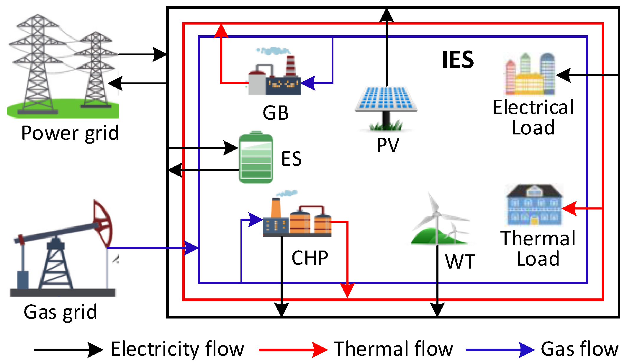
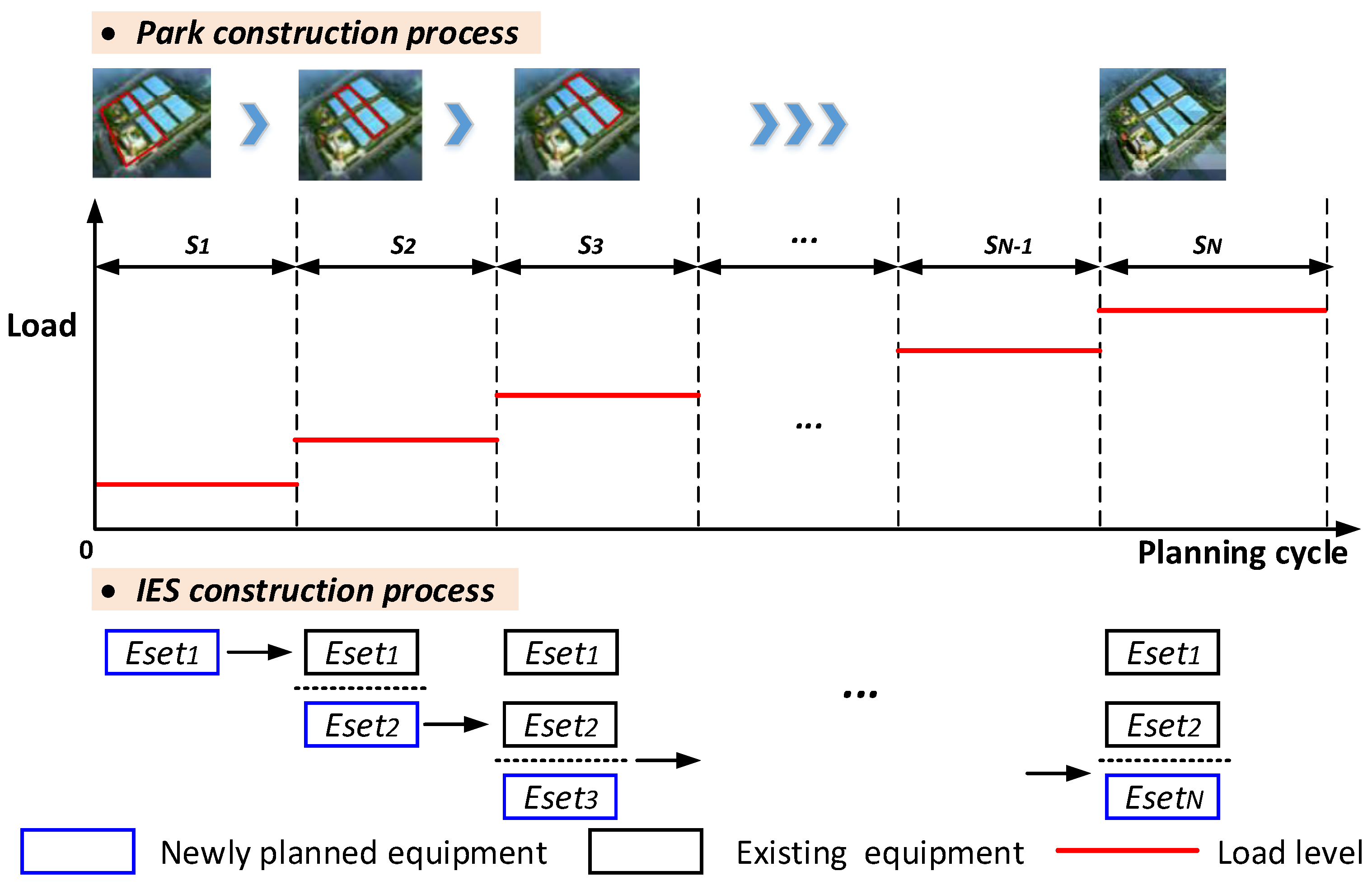
In order to verify the validity and accuracy of the proposed model, the carbon-oriented planning method was applied to a planned IES with CHP, an EB, a ES, PVs, and a WT. The planning period of the IES was 15 years. According to the load growth in the park, it was assumed that the initial load growth rate would be faster; the mid-term load growth rate, lower; and the late-term load level, gradually stabilized.

3.1. Basic Parameters

The planning cycle of the IES was divided into three stages, and the duration of each stage was 3 years, 5 years, and 7 years.

Table 1. Load information on each stage of IES.

Stage	Starting Time	Maximum Electrical Load	Maximum Thermal Load
Stage 1	Year 1	800 kW	800 kW
Stage 2	Year 4	1000 kW	1200 kW
Stage 3	Year 9	1200 kW	1600 kW

shows the load information of each stage of the IES. The economic and technical parameters of the candidate planning equipment are shown in

Table 2. Economic parameters of candidate planning equipment.

Equipment	Investment	Operation Cost	Lifetime
CHP	7000 CNY/kW	0.05 CNY/kW	25 years
GB	1000 CNY/kW	0.04 CNY/kW	25 years
ES	2000 CNY/kW	0.026 CNY/kW	15 years
PV	4500 CNY/kW	0.039 CNY/kW	25 years
WT	5100 CNY/kW	0.025 CNY/kW	25 years

and

Table 3. Technical parameters of candidate planning equipment.

Parameters	Value
Generating efficiency of CHP	0.3
Thermal–electricity ratio of CHP	1.47
Heating efficiency of GB	0.89
Efficiency of waste heat boiler	0.8
Charge/discharge efficiency of ES	0.95/0.95

.

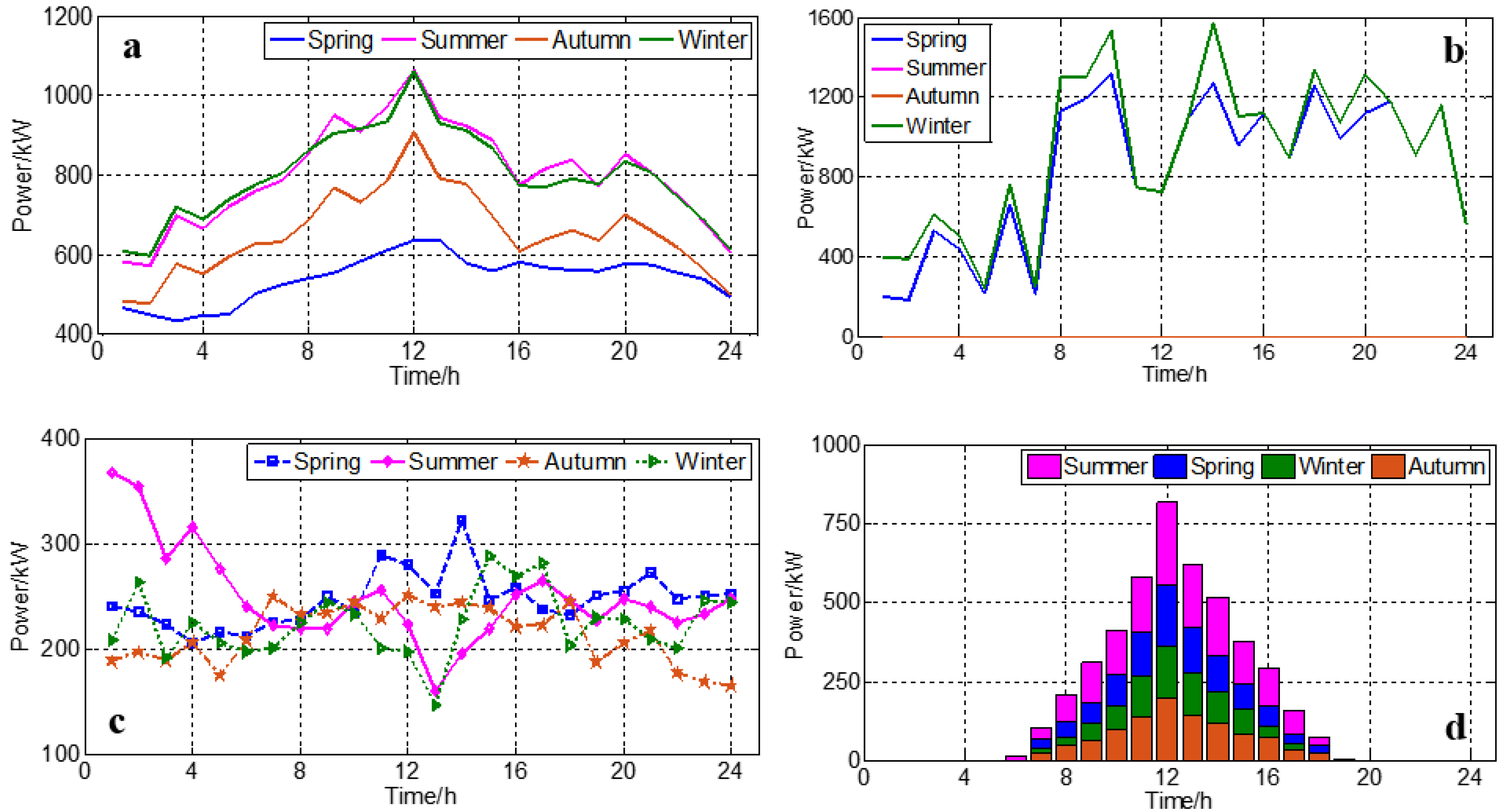
To truly reflect the actual operating conditions of the IES, the data of the electrical load, thermal load, predicted WT power, and predicted PV power of four typical days in spring, summer, autumn, and winter were selected for optimization. Figure 3a,b show the typical daily electrical load and thermal load, respectively. Figure 3c,d show typical daily predicted power curves of the WT and PVs in different seasons, respectively. It is assumed that the prediction error of the WT was 20% and that of the PVs was 15%. The uncertainty adjustment parameters of the WT and PVs are 10 and 8, respectively. The optimal time period was 24 h, and the time interval for each optimization was 1 h.

Table 4. Wholesale electricity prices in the electricity market.

Time Windows	Value
1:00~7:00	0.564 CNY/kWh
8:00~9:00; 14:00~17:00	0.826 CNY/kWh
10:00~13:00; 18:00~24:00	1.134 CNY/kWh

shows the wholesale electricity price in the electricity market. The natural gas price is 3.25 CNY/m³, and the on-grid tariff is 0.45 CNY/kWh. The introductory price of carbon trading is 78.97 CNY/t, the growth coefficient of the trading price is 0.25, and the interval length of the carbon trading price is 80,000 kg. The CEI index of natural gas is 1.96 kg/m³, the CEI index of coal power is 0.85 kg/kWh, and the low-calorific value of natural gas is 9.78 kWh/m³. The carbon emission benchmark for the comprehensive power supply of units is 0.392 kg/kWh, and the thermal–electricity conversion coefficient is 1.25. The electricity input of the IES from the grid is assumed to be coal electricity only.

To illustrate the effectiveness of the established method in improving system operation economy and carbon emission reduction, two scenarios were set for comparison.

Scenario 1: The equipment configuration of the whole planning cycle is planned only at the beginning of the first year, regardless of the IES construction sequence.

Scenario 2: In considering the IES construction sequence, the multi-stage planning method proposed in this paper is adopted to plan the equipment configuration scheme at each stage.

3.2. Simulation Results

In solving the planning schemes of Scenario 1 and Scenario 2, the equipment planning results of each stage can be obtained.

Table 5. Capacity planning results of the IES.

Equipment	Scenario	Stage 1	Stage 2	Stage 3	Total
CHP/kW	Scenario 1	1350	0	0	1350
	Scenario 2	800	350	350	1500
GB/kW	Scenario 1	360	0	0	360
	Scenario 2	150	100	50	300
PV/kW	Scenario 1	260	0	0	260
	Scenario 2	150	150	0	300
WT/kW	Scenario 1	300	0	0	300
	Scenario 2	150	150	100	400
ES/kW	Scenario 1	200	0	0	200
	Scenario 2	100	50	0	150

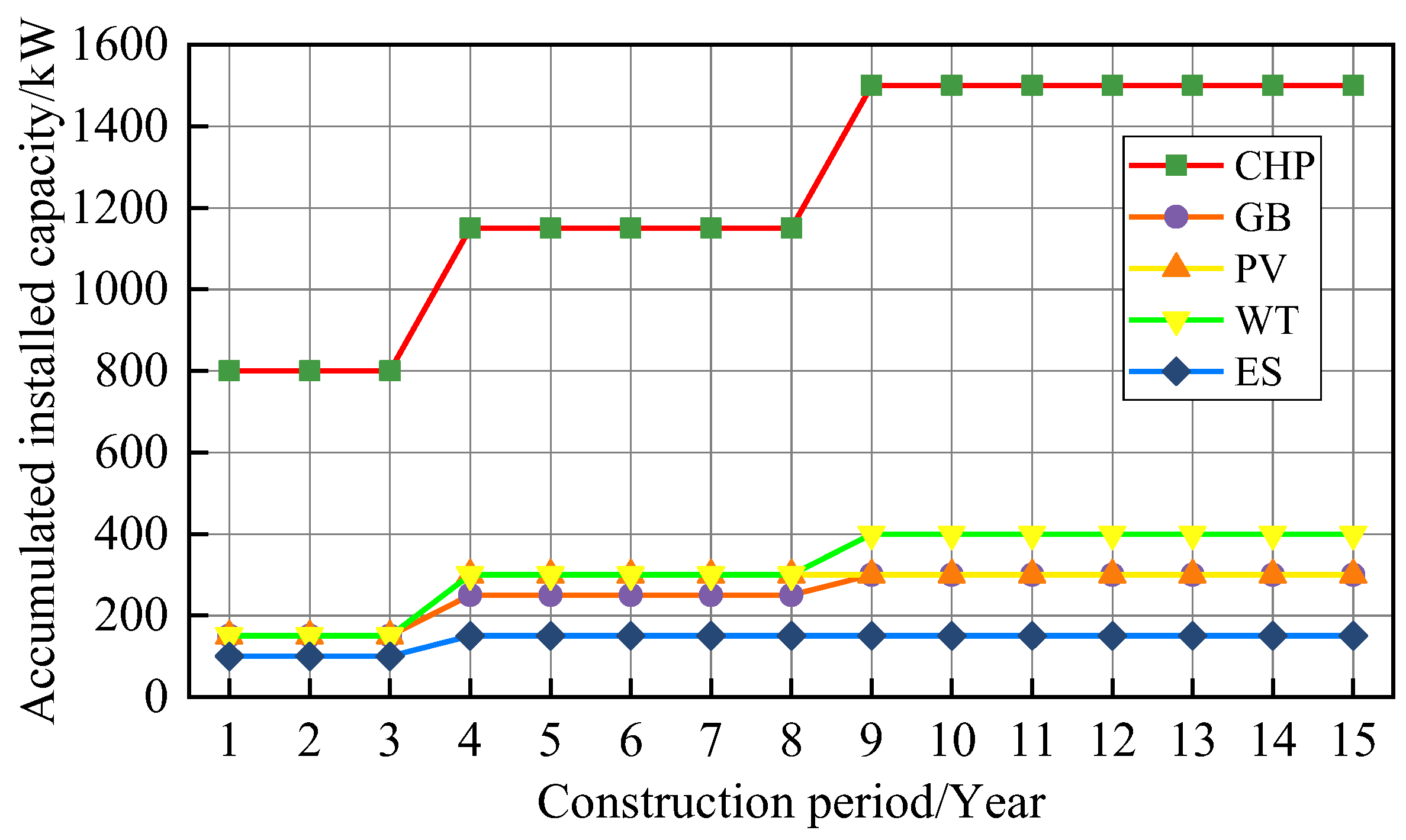
shows the capacity planning result of the IES at different stages. Figure 4 shows the construction time sequence of various equipment.

As shown in the data in Table 5, in the phased planning scenario, the total installed capacities of the CHP and WT were 1500 kW and 400 kW, respectively, which are 11.11% and 33.33% higher than the scenario capacity planned once at the beginning of the year. In the phased planning scenario, the total installed capacities of the GB, PVs, and ES were 300 kW, 200 kW, and 150 kW, respectively, which are 8.33%, 13.33%, and 25.00% lower than the scenario capacity planned once at the beginning of the year. In addition, in analyzing the data changes in Table 5, it can be seen that in the scenario of phased planning, the capacities of the CHP, PVs, and ES are relatively large in the first stage of planning, accounting for more than or equal to 50% of the total capacity, which indicates that this equipment is the primary energy supply equipment in the optimization of system operation.

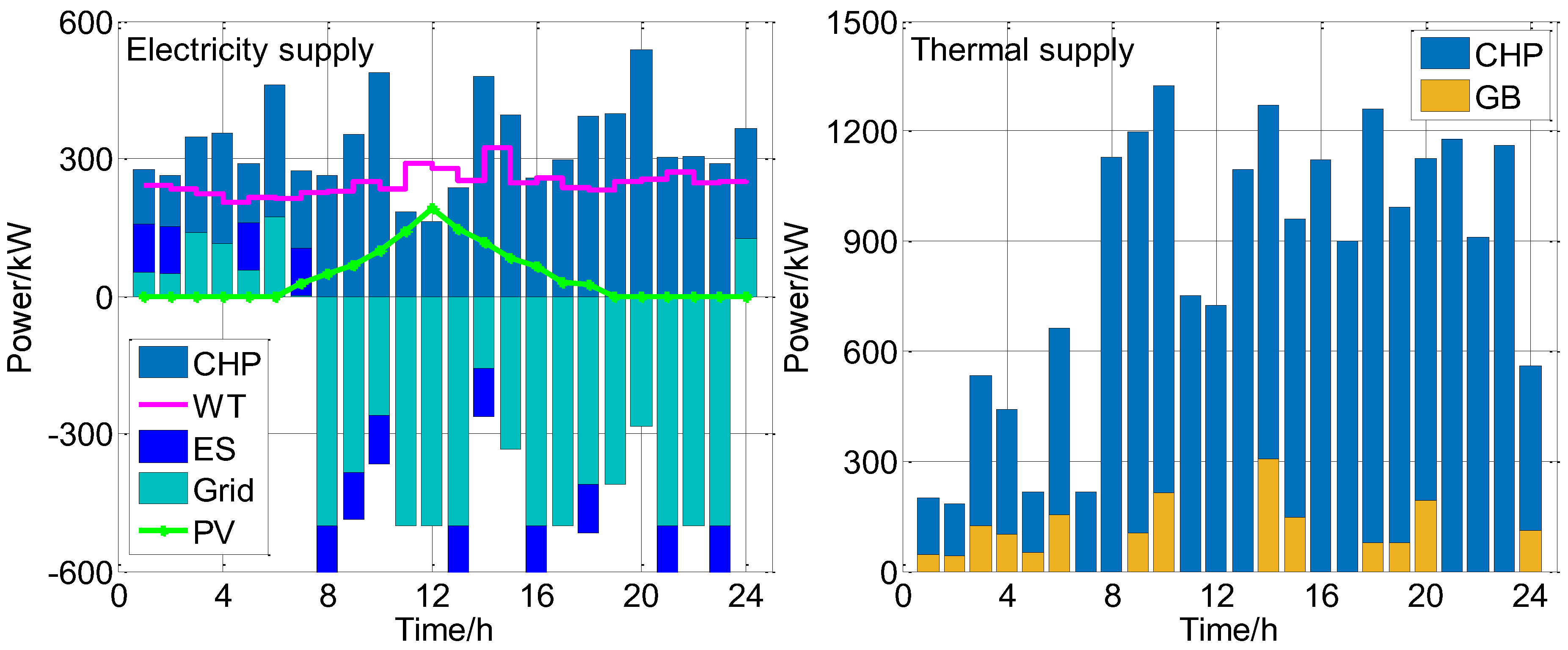
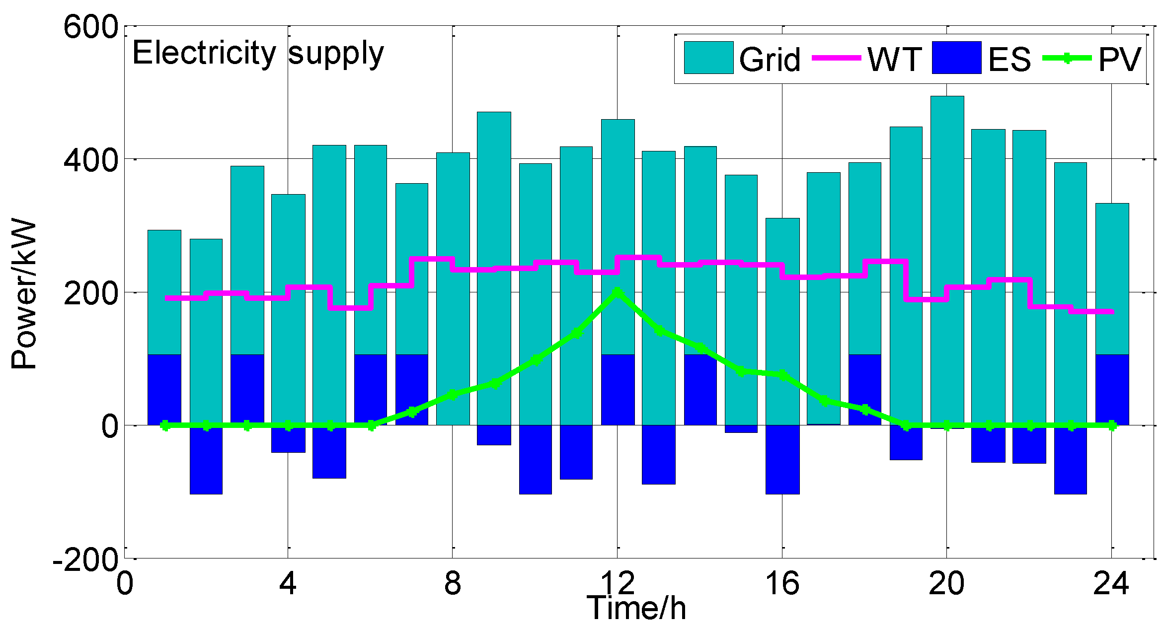
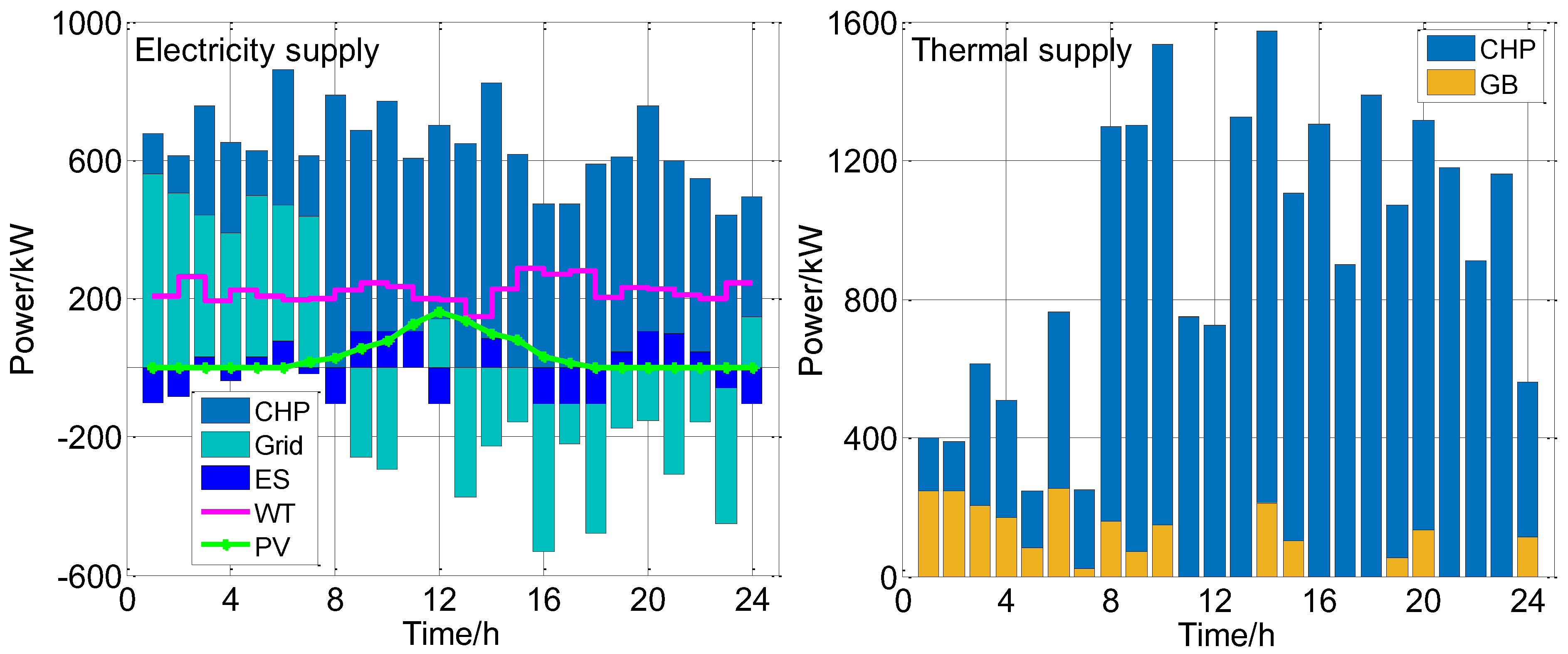
From the perspective of the constructed time sequences, the planned capacity of the PVs and ES reaches saturation in the second stage, while the planned capacity of the CHP, GB, and WT reaches saturation in the third stage. To further analyze the operational status of the system in a phased planning scenario, we simulated the operating conditions of the system in all four seasons when the planned capacity of the equipment in this scenario reached saturation. Figure 5, Figure 6, Figure 7 and Figure 8 show the dispatching strategy of the energy supply equipment in the spring, summer, autumn, and winter.

Based on the above simulation results, the calculation results of the operation economy, renewable energy utilization rate, and carbon emissions were obtained.

Table 6. Life cycle cost of IES in different scenarios.

Composition of Cost	Scenario 1	Scenario 2
Investment cost/10,000 CNY	1295.000	1286.000
Electricity cost/10,000 CNY	6832.800	5978.700
Maintenance cost/10,000 CNY	908.250	886.727
Battery degradation cost/10,000 CNY	85.410	76.869
Fuel consumption cost/10,000 CNY	8634.951	7443.482
Carbon trading cost/10,000 CNY	−70.058	−91.902
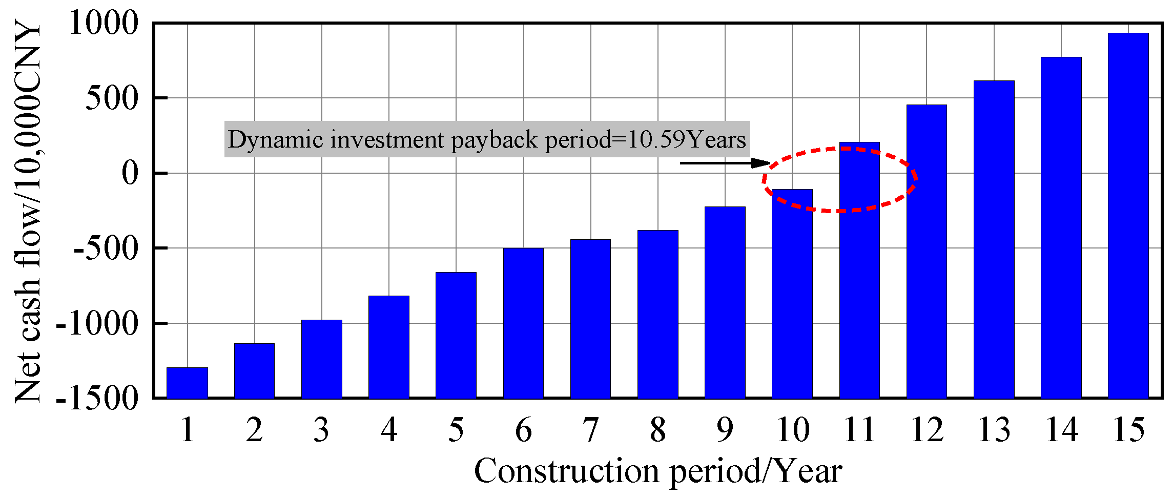
Total cost/10,000 CNY	17,686.353	15,579.875

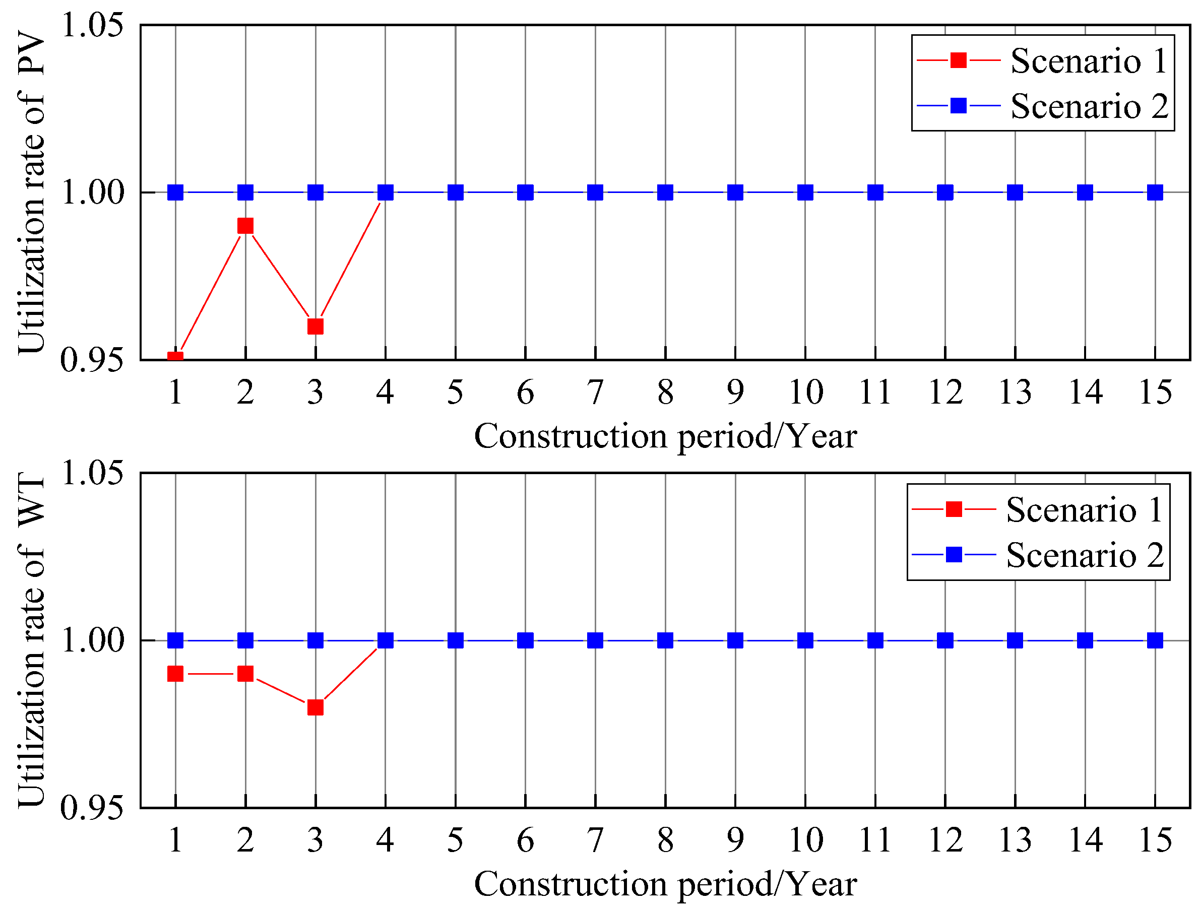
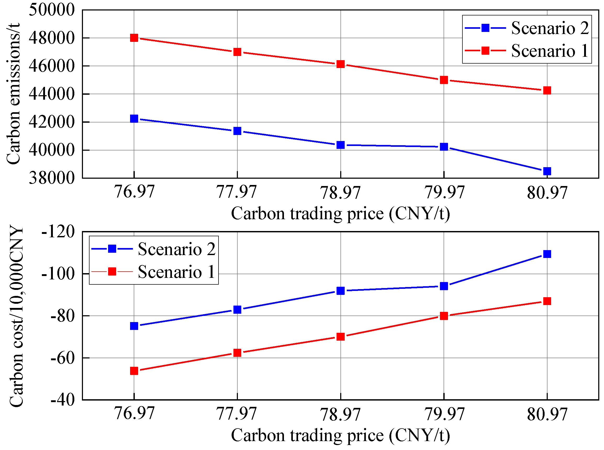
shows the life cycle cost of the IES in different scenarios, and Figure 9 shows the variation trend of the accumulated net cash flow with the life cycle. Figure 10 shows the energy utilization rate of the PVs and WT in different scenarios, and Figure 11 shows the carbon emission changing with the change in carbon trading prices.

In order to further verify the advantages of the model considering the carbon quota in improving economy and carbon emission reduction, the proposed model in this paper and other models that consider the carbon cost in their objective function were compared. The models and parameters used in the simulation are consistent with this paper, but the carbon cost model refers to Ref. [34], and the carbon cost coefficient, like the basic price of carbon trading, was 78.97 CNY/t. The difference between the two models above is that the model established in this paper can participate in carbon quota trading to flexibly adjust carbon emissions and carbon costs, while the model in Ref. [34] can solve only the problem of excessive carbon emission by paying carbon emission costs.

Table 7. Simulation results of two models.

Composition of Cost	Model in Ref. [34]	Model in This Paper
Investment cost/10,000 CNY	1289.000	1286.000
Electricity cost/10,000 CNY	6123.590	5978.700
Maintenance cost/10,000 CNY	899.260	886.727
Battery degradation cost/10,000 CNY	79.265	76.869
Fuel consumption cost/10,000 CNY	8016.390	7443.482
Carbon cost/10,000 CNY	16.355	−91.902
Total cost/10,000 CNY	16,423.860	15,579.875

shows the simulation results of the two models.

As can be seen from the data in Table 7, the model established in this paper has more advantages than the model in Ref. [34] in reducing the total cost and carbon cost. The model in Ref. [34] has no flexible mechanism with which to participate in carbon trading because it does not consider the carbon quota. As a result, the system is always subject to strict constraints of carbon emission during operation, and it is impossible to flexibly adjust the carbon emission strategy without carbon quota trading. In some cases of excessive carbon emission, only a high carbon cost can be paid. The model established in this paper can gain profits by trading surplus carbon quota flexibly. The numerical simulation results show that the total cost of the model established in this paper is 5.14% lower than that of the model in Ref. [34].

3.3. Result Analysis

To further illustrate the significant effects of phased planning in improving operational efficiency and reducing carbon emissions. This section analyzes the full lifecycle cost, renewable energy utilization efficiency, and carbon emissions of the IES in two planning scenarios [12,13,14,15,16,17,18].

Compared with the scenario of completing planning at the beginning of the life cycle at one time, the low carbon-oriented capacity optimization method considering construction time sequence and uncertainty can reduce the cost of the integrated energy system. According to the data in Table 6, the total system costs for Scenario 1 and Scenario 2 were CNY 176.86353 million and CNY 155.79875 million, respectively. The total cost of phased planning was reduced by 11.91% compared to the total cost of one-time planning at the beginning of the year. Among them, the system capacity planning cost in Scenario 2 was CNY 12.86 million, 0.69% lower than that of one-time planning. In addition, the carbon trading returns of the system in two scenarios were CNY 7,005,800 and CNY 9,190,200, respectively, indicating that the carbon emissions in the system did not exceed the carbon quota in both scenarios. From Figure 9, it can be seen that in the phased planning scenario, the dynamic investment payback period of the investment is 10.59 years, achieving a balance between income and expenditure.

Compared with the scenario of completing planning at the beginning of the life cycle at one time, the low carbon-oriented capacity optimization method considering construction time sequence and uncertainty can enhance renewable energy utilization. From Figure 10, it can be seen that the average utilization rates of PV and WT power in the first stage of Scenario 1 were 96.67% and 98.67%, respectively, indicating the presence of PV and WT electricity abandonment phenomena. The reason for these phenomena is that in Scenario 1, all equipment was planned as disposable cups, and the load level of the IES has not yet reached its peak, resulting in the PV and WT power generation not being fully utilized. On the other hand, in Scenario 2, as both the PV and WT power were planned in stages, the matching degree between their power generation and load are relatively high, resulting in a utilization rate of 100% for both PV and WT power throughout their entire lifecycle.

Compared with the scenario of completing planning at the beginning of the life cycle at one time, the low carbon-oriented capacity optimization method considering construction time sequence and uncertainty can reduce system carbon emissions. Figure 11 shows the carbon emission and carbon trading cost changes with the changes in carbon trading prices. Due to the consideration of system carbon quotas and carbon emission factors during the planning phase, and the consideration of carbon trading costs in the optimization objective function, the carbon emissions of the system never exceeded the standard. Therefore, when the carbon trading price changes, the changes in the system carbon emissions and carbon trading costs are relatively small.

Based on the above analysis, the method established in this paper can be applied in the practical engineering of equipment capacity planning and the low-carbon operation optimization of IESs to reduce the cost and carbon emission of the systems at the planning stage as much as possible and improve the utilization rate of renewable energy. In addition, the current research focused only on optimizing the energy system capacity and did not consider the choice of equipment construction location. In the future, the low-carbon-oriented capacity and location optimization methods can be considered and studied.

4. Conclusions

This study focused on the low-carbon-oriented capacity optimization of an electric–thermal IES by considering construction time sequence and uncertainty, and through simulations and analyses, some important conclusions were obtained. (1) The established method can effectively reduce the cost of the system; the total cost of phased planning was reduced by 11.91% compared to the total cost of one-time planning at the beginning of the year. (2) The established method can effectively enhance the renewable energy utilization of the system compared to the one-time planning method; the utilization rate of both PV and WT power can reach 100%. (3) The established method can effectively reduce the carbon emissions of the system compared to the one-time planning method; the carbon emissions of the system decreased by 23.77%. (4) The numerical simulation results show that the total cost of the model established in this paper was 5.14% lower than that of the model considering the carbon cost in the objective function. To sum up, compared with the scenario of completing planning at the beginning of the life cycle at one time, the proposed low-carbon-oriented capacity optimization method that considers construction time sequence and uncertainty can not only reduce the cost of integrated energy system, but also help to enhance renewable energy utilization and reduce system carbon emissions.

References

1. Wang, R.; Wen, X.; Wang, X.; Fu, Y.; Zhang, Y. Low carbon optimal operation of integrated energy system based on carbon capture technology, LCA carbon emissions and ladder-type carbon trading. Appl. Energy 2022, 311, 118664. [Google Scholar] [CrossRef]
2. Wang, Y.; Wang, Y.; Huang, Y.; Yu, H.; Du, R.; Zhang, F.; Zhang, F.; Zhu, J. Optimal Scheduling of the Regional Integrated Energy System Considering Economy and Environment. IEEE Trans. Sustain. Energy 2019, 10, 1939–1949. [Google Scholar] [CrossRef]
3. Xing, X.; Tsinghua University; Lin, J.; Song, Y.; Zhou, Y.; Mu, S.; Hu, Q.; National Institute of Clean and Low Carbon Energy. Tsinghua-Sichuan Energy Internet Research Institute Modeling and operation of the power-to-gas system for renewables integration: A review. CSEE J. Power Energy Syst. 2018, 4, 168–178. [Google Scholar] [CrossRef]
4. Zhang, D.; Zhu, H.; Zhang, H.; Goh, H.W.; Liu, H.; Wu, T. An optimized design of residential integrated energy system considering the power-to-gas technology with multi-functional characteristics. Energy 2022, 238, 121774. [Google Scholar] [CrossRef]
5. Li, L.; Wang, J.; Zhong, X.; Lin, J.; Wu, N.; Zhang, Z.; Meng, C.; Wang, X.; Shah, N.; Brandon, N.; et al. Combined multi-objective optimization and agent-based modeling for a 100% renewable island energy system considering power-to-gas technology and extreme weather conditions. Appl. Energy 2021, 308, 118376. [Google Scholar] [CrossRef]
6. Liu, Y.; Liu, T. Research on System Planning of Gas-Power Integrated System Based on Improved Two-Stage Robust Optimi-zation and Non-Cooperative Game Method. IEEE Access 2021, 9, 79169–79181. [Google Scholar] [CrossRef]
7. Zhang, Z.; Wang, C.; Lv, H.; Liu, F.; Sheng, H.; Yang, M. Day-Ahead Optimal Dispatch for Integrated Energy System Considering Power-to-Gas and Dynamic Pipeline Networks. IEEE Trans. Ind. Appl. 2021, 57, 3317–3328. [Google Scholar] [CrossRef]
8. Cui, Y.; Xu, Y.; Huang, T.; Wang, Y.; Cheng, D.; Zhao, Y. Low-carbon economic dispatch of integrated energy systems that incorporate CCPP-P2G and PDR considering dynamic carbon trading price. J. Clean. Prod. 2023, 423, 138812. [Google Scholar] [CrossRef]
9. Pan, G.; Gu, W.; Lu, Y.; Qiu, H.; Lu, S.; Yao, S. Optimal Planning for Electricity-Hydrogen Integrated Energy System Considering Power to Hydrogen and Heat and Seasonal Storage. IEEE Trans. Sustain. Energy 2020, 11, 2662–2676. [Google Scholar] [CrossRef]
10. Guo, X.; Lou, S.; Wu, Y.; Wang, Y. Low-Carbon Operation of Combined Heat and Power Integrated Plants Based on Solar-Assisted Carbon Capture. J. Mod. Power Syst. Clean Energy 2021, 10, 5. [Google Scholar] [CrossRef]
11. Guo, X.; Lou, S.; Wu, Y.; Wang, Y. Low-carbon optimal planning of an integrated energy station considering combined power-to-gas and gas-fired units equipped with carbon capture systems. Int. J. Electr. Power Energy Syst. 2022, 138, 107966. [Google Scholar]
12. He, S.; Gao, H.; Wang, L.; Xiang, Y.; Liu, Y.Y. Distributionally robust planning for integrated energy systems incorporating electric-thermal demand response. Energy 2020, 213, 118783. [Google Scholar] [CrossRef]
13. Cao, Y.; Wei, W.; Wang, J.; Mei, S.; Shafie-Khah, M.; Catalao, J.P.S. Capacity Planning of Energy Hub in Multi-Carrier Energy Networks: A Data-Driven Robust Stochastic Programming Approach. IEEE Trans. Sustain. Energy 2020, 11, 3–14. [Google Scholar] [CrossRef]
14. Daniel, O.; Pourakbari, M.; Mantovan, J. Adaptive Robust Short-Term Planning of Electrical Distribution Systems Considering Siting and Sizing of Renewable Energy Based DG Units. IEEE Trans. Sustain. Energy 2019, 10, 158–169. [Google Scholar]
15. Pan, G.; Gu, W.; Zhou, S.; Wu, Z.; Qiu, H.; Lu, Y. Synchronously decentralized adaptive robust planning method for multi-stakeholder integrated energy systems. IEEE Trans. Sustain. Energy 2020, 11, 1128–1139. [Google Scholar] [CrossRef]
16. Ge, L.; Liu, H.; Yan, J.; Zhu, X.; Zhang, S.; Li, Y. Optimal Integrated Energy System Planning with DG Uncertainty Affine Model and Carbon Emissions Charges. IEEE Trans. Sustain. Energy 2021, 13, 905–918. [Google Scholar] [CrossRef]
17. Li, C.; Wang, N.; Wang, Z.; Dou, X.; Zhang, Y.; Yang, Z.; Maréchal, F.; Wang, L.; Yang, Y. Energy hub-based optimal planning framework for user-level integrated energy systems: Considering synergistic effects under multiple uncertainties. Appl. Energy 2021, 307, 118099. [Google Scholar] [CrossRef]
18. Lei, Y.; Wang, D.; Jia, H.; Li, J.; Chen, J.; Li, J.; Yang, Z. Multi-stage stochastic planning of regional integrated energy system based on scenario tree path optimization under long-term multiple uncertainties. Appl. Energy 2021, 300, 117224. [Google Scholar] [CrossRef]
19. Tan, Q.; Ding, Y.; Ye, Q.; Mei, S.; Zhang, Y.; Wei, Y. Optimization and evaluation of a dispatch model for an integrated wind-photovoltaic-thermal power system based on dynamic carbon emissions trading. Appl. Energy 2019, 253, 113598. [Google Scholar] [CrossRef]
20. Wang, Y.; Hu, J. Energy Management in Integrated Energy System Using Energy–Carbon Integrated Pricing Method. IEEE Trans. Sustain. Energy 2023, 14, 1992–2005. [Google Scholar] [CrossRef]
21. Wang, Z.; Shi, Y.; Tang, Y.; Men, X.; Cao, J.; Wang, H. Low Carbon Economy Operation and Energy Efficiency Analysis of Integrated Energy Sys-tems Considering LCA Energy Chain and Carbon Trading Mechanism. Proc. CSEE 2019, 39, 1614–1626. [Google Scholar]
22. Huang, Y.; Wang, Y.; Liu, N. Low-carbon economic dispatch and energy sharing method of multiple Integrated Energy Systems from the perspective of System of Systems. Energy 2022, 244, 122717. [Google Scholar] [CrossRef]
23. Cheng, Y.; Zhang, N.; Zhang, B.; Kang, C.; Xi, W.; Feng, M. Low-Carbon Operation of Multiple Energy Systems Based on Energy-Carbon Integrated Prices. IEEE Trans. Smart Grid 2019, 11, 1307–1318. [Google Scholar] [CrossRef]
24. Li, Y.; Zou, Y.; Tan, Y.; Cao, Y.; Liu, X.; Shahidehpour, M.; Tian, S.; Bu, F. Optimal Stochastic Operation of Integrated Low-Carbon Electric Power, Natural Gas, and Heat Delivery System. IEEE Trans. Sustain. Energy 2019, 9, 273–283. [Google Scholar] [CrossRef]
25. Jiang, T.; Deng, H.; Bai, L.; Zhang, R.; Li, X.; Chen, H. Optimal energy flow and nodal energy pricing in carbon emission-embedded integrated energy systems. CSEE J. Power Energy Syst. 2018, 4, 179–187. [Google Scholar] [CrossRef]
26. Wang, Y.; Qiu, J.; Tao, Y.; Zhao, J. Carbon-Oriented Operational Planning in Coupled Electricity and Emission Trading Markets. IEEE Trans. Power Syst. 2020, 35, 3145–3157. [Google Scholar] [CrossRef]
27. Zhang, J.; Liu, Z. Low carbon economic scheduling model for a park integrated energy system considering integrated demand response, ladder-type carbon trading and fine utilization of hydrogen. Energy 2024, 130311. [Google Scholar] [CrossRef]
28. Lei, D.; Zhang, Z.; Wang, Z.; Zhang, L.; Liao, W. Long-term, multi-stage low-carbon planning model of electricity-gas-heat integrated energy system considering ladder-type carbon trading mechanism and CCS. Energy 2023, 280, 128113. [Google Scholar] [CrossRef]
29. Zhang, H.; Wu, Q.; Chen, J.; Lu, L.; Zhang, J.; Zhang, S. Multiple stage stochastic planning of integrated electricity and gas system based on dis-tributed approximate dynamic programming. Energy 2023, 270, 126892. [Google Scholar] [CrossRef]
30. Wang, Z.; Wang, Y.; Ji, H.; Hasanien, H.M.; Zhao, J.; Yu, L.; He, J.; Yu, H.; Li, P. Distributionally robust planning for data center park considering operational economy and reliability. Energy 2024, 290, 130185. [Google Scholar] [CrossRef]
31. Wang, Z.; Wu, F.; Li, Y.; Li, J.; Liu, Y.; Liu, W. Day-ahead dispatch approach for cascaded hydropower-photovoltaic complementary system based on two-stage robust optimization. Energy 2023, 265, 126145. [Google Scholar] [CrossRef]
32. Huang, S.; Liu, K.; Zhang, Z.-H. Column-and-constraint-generation-based approach to a robust reverse logistic network design for bike sharing. Transp. Res. Part B Methodol. 2023, 173, 90–118. [Google Scholar] [CrossRef]
33. Wu, M.; Xu, J.; Zeng, L.; Li, C.; Liu, Y.; Yi, Y.; Wen, M.; Jiang, Z. Two-stage robust optimization model for park integrated energy system based on dynamic programming. Appl. Energy 2022, 308, 118249. [Google Scholar] [CrossRef]
34. Guo, W.; Liu, P.; Shu, X. Optimal dispatching of electric-thermal interconnected virtual power plant considering market trading mechanism. J. Clean. Prod. 2020, 279, 123446. [Google Scholar] [CrossRef]
Figure 1. Typical system structure of electric–thermal IES.
Processes 12 00648 g001
Figure 2. Schematic of park IES’s multi-stage planning considering CTS.
Processes 12 00648 g002
Figure 3. Predicted power curves of the electrical load, thermal load, WT, and PVs. (a) electrical load; (b) thermal load; (c) WT power (d) PVs power.
Processes 12 00648 g003
Figure 4. Construction time sequences of various equipment.
Processes 12 00648 g004
Figure 5. Dispatching strategy of energy supply equipment in spring.
Processes 12 00648 g005
Figure 6. Dispatching strategy of energy supply equipment in summer.
Processes 12 00648 g006
Figure 7. Dispatching strategy of energy supply equipment in autumn.
Processes 12 00648 g007
Figure 8. Dispatching strategy of energy supply equipment in winter.
Processes 12 00648 g008
Figure 9. Variation trend of accumulated net cash flow with the life cycle.
Processes 12 00648 g009
Figure 10. Energy utilization rate of PV and WT power in different scenarios.
Processes 12 00648 g010
Figure 11. Carbon emissions change with the change in carbon trading prices.
Processes 12 00648 g011