Research on an Optimal Maintenance and Inventory Model Based on Carbon Tax Policy

Abstract

The equipment in a factory will gradually deteriorate during production, leading to the production of defective products. Without appropriate maintenance, the defect rate will increase over time. Consequently, the production cost will rise, the inventory quality will be affected, the profit will decrease, and the risk of carbon emissions will increase, leading to more customer complaints and damaging the corporate image. In addition to focusing on preventive maintenance to ensure the quality of products, companies should also take carbon emissions into consideration. Furthermore, the frequency of maintenance must be carefully considered, as both carbon emissions and maintenance costs will increase if the frequency is too high; conversely, if the maintenance frequency is too low or non-existent, the defect rate may increase cumulatively, or production may be suspended due to equipment failure. Therefore, this research explores preventive maintenance and inventory management issues within an imperfect production system and develops an extended economic production quantity model that incorporates defective products as well as taking carbon tax and preventive maintenance into consideration. The main purpose is to determine the optimal maintenance frequency, production, and replenishment cycle length, so as to maximize the total profit under the carbon tax policy. This study demonstrates a computing process with relatively impractical product data based on the actual business situation of a disposable diaper manufacturer. Furthermore, a sensitivity analysis is implemented to the model parameters in the proposed model. The managemental insights are illustrated based on the results of theoretical analysis to provide a reference to policy makers during decision making, hence, to secure the sustainability and green transitions of corporates. The results of this study not only help to reduce environmental impact but can also improve the competitiveness and sustainable development of enterprises.

1. Introduction

According to the Global Risks Report issued by the World Economic Forum (WEF) in 2022, four out of the five most-possible crises are related to global warming and extreme climates. Carbon emissions are generally considered the major cause of global climate change and this threat has increased gradually. Therefore, numerous policies and activities have been planned in order to inhibit the amount of greenhouse gas emissions. These policies include the development of alternative energy or renewable energy—such as solar power and wind power—establishing the regulation of carbon reductions, promoting the carbon trading market, imposing carbon tax, and building a carbon offset system. These policies and activities will affect the operations of corporate companies. Therefore, if corporations make an operational decision without considering their greenhouse gas emissions, the survival and development of that corporation could be negatively affected due to the underestimated external costs.

In addition, quality management is a crucial issue within businesses, supply chains, and inventory management. The conventional literature on economic order quantity (EOQ) or economic production quantity (EPQ) normally assumes that production systems are complete, hence, the products are effective. Defective products can appear due to negligence in the process controls, human negligence, aging of the equipment, or negligence during transportation [1]. As an example of manufacturing disposable diapers, the safety, functionality, and appearance are all taken into consideration before production. Each material used in the disposable diaper has different characteristics and is stacked together like a sandwich to create a multiplicative effect that prevents leaks. The materials of the disposable diaper can be easily scratched by external forces, or the quality yield can be affected by an offset of the conveyor belt parts during manufacturing and transportation. Once the equipment in the manufacturing process slowly deteriorates and deviates from the process control center line over time, the defect rate will gradually increase, leading to a decrease in production efficiency and affecting inventory. Preventive maintenance is necessary in order to avoid the escalating costs and unnecessary waste resulting from equipment deterioration. Besides deterioration, there still exists the random risk of malfunctions caused by factors such as human negligence or ineffective quality management, which can lead to an increase or underestimation of actual costs. Therefore, under the condition of minimizing the expected unit time cost, it is essential to develop a sufficient preventive maintenance policy including the implementation conditions, an adequate threshold, and an appropriate frequency to avoid unnecessary waste caused by excessive preventive maintenance.

Based on the context discussed above, as corporations aim to maintain efficiency and quality in manufacturing, it is helpful to incorporate the frequency of equipment maintenance and carbon emissions into the EOQ/EPQ model to minimize the carbon emissions and impact on the environment. This is crucial and necessary for corporations, especially during this green transition and sustainability transformation. Therefore, this research assumes that equipment maintenance is available during production, carbon tax policy has been considered, an imperfect production system is employed, and the defect rate varies. This aids in determining sufficient production–inventory-period lengths and the frequency of preventive maintenance needed in order to maximize the total profit per unit time under the carbon tax policy based on the EPQ model. Specifically, the problems to be solved by the proposed model are as follows: (1) in the production process, how to decide whether to perform maintenance and how to determine the optimal frequency of maintenance once maintenance becomes an option? (2) what is the correlation between maintenance and carbon-emission-reduction policies? Moreover, this research develops an algorithm to calculate the sufficient restock-period length and times of maintenance based on an established model. The computing process is demonstrated using an impractical data example faced by a manufacturer of disposable diapers and we discuss the sensitivity analysis of the model’s parameters to illustrate the effect of these parameters on sufficient decisions and the total profit. This aims to provide a reference for determining preventive maintenance and inventory decisions within the corporate framework.

In summary, the main contributions of this research are as follows: First, this study considers the option of preventive maintenance during the production process, which has not been proposed in the previous EPQ model. Secondly, carbon-emission reduction in manufacturing processes is currently an important issue for enterprises and the proposed model provides enterprises with appropriate maintenance decisions, which will achieve the effect of carbon-emission reductions by reducing product defect rates. Additionally, we use disposable diaper manufacturing as an example and conduct numerical analysis using data consistent with the manufacturer’s actual situation to make the model more practical.

The rest of this paper is organized as follows: Section 2 focuses on the review of previous relevant studies. Section 3 develops the mathematical model, including carbon tax and preventive maintenance, and then explains the theoretical results and solution process. Furthermore, a real case and numerical examples are presented to illustrate the solution procedure, and a sensitivity analysis is performed to provide some managerial insights in Section 4. Finally, Section 5 concludes this study and provides management revelations and directions for future research.

2. The Literature Review

This section reviews the literature discussing economic production quantity models that incorporate carbon emissions and equipment maintenance management.

2.1. Economic Production Quantity Models with Carbon Emissions

Since the EOQ model was proposed by Harris [2], it has been widely used as a foundation for discussions relating to the inventory model. Taft [3] developed the EPQ based on the model proposed by [2]; however, some assumptions by Taft [3], such as perfect production processes and a 100% yield rate, were too optimistic. Equipment deterioration or other random factors during production processes will produce defective products and decrease the production rate, thus affecting inventory decision-making. The effect on the inventory model caused by an imperfect production system with a defective product was first proposed by Porteus [4]. Salameh and Jaber [5] extended the conventional EPQ/EOQ model and proposed a solution in which defective products can be sold at a discount after full inspection. Chiu [6] discussed the effect of the conventional EPQ model with a defective product. Khan et al. [7] built an EPQ model with sufficient production and order quantities by adding an inspection error to Salameh and Jaber’s [5] model. Yuan et al. [8] focused on the inventory system based on the EPQ model with random defective products and adjustable production rates. They proposed a solution to decrease the impact of random defective products during production processes on inventory systems by adjusting the production rate.

The effect of carbon emissions on the EPQ model has been widely discussed recently. Taleizadeh et al. [9] proposed four sustainable EPQ models, considering stockout situations in the production system. Daryanto and Wee [10] proposed an EPQ model considering carbon emissions and assumed that stockouts occur as well as complete backorders. Moreover, Daryanto and Wee [11] proposed an EPQ model considering defective products and carbon tax, which allowed defective products to be sold on the secondary market. Sinha and Modak [12] suggested plantation as a solution to the carbon-emission issue and compared the results with or without plantation using empirical data. Fadlil et al. [13] proposed an EPQ model considering refunded products, unused products, the remaking of defective products, and carbon-emission costs. Gharaei et al. [14] developed an EPQ model considering carbon-emission costs under the green transition policy. Karim et al. [15] conducted a systematic literature review on the sustainable EPQ model including carbon emissions and product recycling. Recently, to cope with extreme climate issues, Paul et al. [16] formulated an (EPQ) model with an investment in green operations and deterioration. Although low-carbon investment issues are beginning to be considered in EPQ models, there is no production–inventory-related literature to reduce carbon emissions from equipment maintenance to reduce defect rates. During the production process, if preventive maintenance can be performed before the equipment becomes out of control, it will not only help reduce the waste from defective products but also reduce carbon emissions.

2.2. Inventory Models with Equipment Maintenance

Cassady et al. [17] proposed a trade-off relationship between equipment maintenance and product quality and demonstrated that using both methods is better than single usage. Wang [18] categorized preventive maintenance policy as follows: age-dependent preventive maintenance policy, periodic preventive maintenance, failure limit policy, sequential preventive maintenance policy, repair limit policy, repair time counting, and reference time policy. Kim et al. [19] proposed two periodic preventive maintenance policies, namely type I and type II, which aim to find a sufficient preventive maintenance policy to minimize expected cost rates by computing the expected cost rate within a product’s lifecycle in each preventive maintenance policy. Schutz et al. [20] proposed periodic and sequential preventive maintenance policies over a finite planning horizon, in which the periodic preventive maintenance policy aims to ensure sufficient time for periodic preventive maintenance, and where the sequential preventive maintenance policy computes the sufficient number and duration of preventive maintenance intervals. Lin and Wang [21] proposed a genetic algorithm to optimize the periodic preventive maintenance policy in a series-parallel system. Liu et al. [22], concurrently, integrated non-cyclical preventive maintenance and tactical production planning into a multi-unit production system that processes non-cyclical preventive maintenance at the end of a product’s lifecycle and processes corrective maintenance at failure. Mazidi et al. [23] built a useful maintenance model by combining corrective and preventive maintenance policies. Yang et al. [24] proposed a periodic and opportunistic preventive maintenance policy in which the periodic preventive maintenance policy focuses on defects due to deterioration and opportunistic preventive maintenance policy aims for the sufficient distribution of maintenance resources, especially for production wait times caused by a shortage of requirements and being out of material. Wu et al. [25] divided maintenance into two stages: An inspection with a limited time to monitor the defects and process the incomplete preventive maintenance at the first stage. The complete maintenance will be processed at a scheduled time or at an opportunistic production wait time in the second stage. Resources can be flexibly distributed with each stage.

2.3. Research Gap

Based on the aforementioned relevant literature, although inventory management models that consider imperfect production systems including preventive maintenance have been proposed, there has not yet been a sustainable inventory model that considers the defect rate to be time-dependent and can consider maintenance options. In addition, the previous literature has not discussed the production and inventory management issues of the disposable diaper manufacturer. Thus, there is a research gap in the literature regarding the optimal production and maintenance decisions of the disposable diaper manufacturer based on carbon-emission policy.

3. Method

In this section, we apply an extended economic production quantity model to an imperfect production system that takes both carbon tax and preventive maintenance into consideration. First, before developing the proposed model, the notation and assumptions used will be illustrated; then, the model of this study will be derived, and the solution process will be explained.

3.1. Notation and Assumptions

The symbols in

Table 1. Symbols’ descriptions.

Symbol	Symbol’s Description
P	Production rate
D	Demand rate
a	Fixed defect rate parameter
b	Variable defect rate parameter
S	Setup cost
$\widehat{S}$	Carbon emissions generated by the setup activity
v	Unit production cost
$\widehat{v}$	Unit carbon emissions from product production
h	Unit holding cost per unit time
$\widehat{h}$	Unit carbon emissions per unit time from product storage
k	Maintenance cost
$\widehat{k}$	Carbon emissions generated by maintenance activity
$u_b$	Carbon tax per unit of carbon emissions
s	Unit sales price
$t_1$	Production cycle length, a decision variable
$T$	Replenishment cycle length, a decision variable
n	Number of maintenance operations during the production period, a decision variable
$t_a$	$\mathrm{Time}\mathrm{intervals}\mathrm{between}\mathrm{each}\mathrm{maintenance}\mathrm{check},\mathrm{where}{0\le t}_a\le t_1$
$u\left(t\right)$	$\mathrm{Defect}\mathrm{rate}\mathrm{at}\mathrm{time}\mathrm{in}\mathrm{each}\mathrm{maintenance}\mathrm{cycle},\mathrm{a}\mathrm{function}\mathrm{that}\mathrm{increases}\mathrm{with}\mathrm{time}. \mathrm{That}\mathrm{is},\left(t\right)=a+bt,$$\mathrm{where}0\le t\le t_a$
$TP(t_1,n,T)$	Total profit function per unit time

are used in this research to develop the model.

Next, to facilitate the development of the model, this study requires the following assumptions:

• This inventory system focuses on a single product of a single manufacturer within an infinite planning horizon;
• During the production period, the defect rate will increase over time and can be restored to the original level through maintenance with time interval $t_a$. That is, the defect rate within one maintenance cycle at time t is $u\left(t\right)=a+bt$, where $0\le t\le t_a$;
• It is assumed that the production rate of good products is greater than the demand rate within the replenishment cycle, which implies $\left[1-u\left(t\right)\right]P>D$; otherwise, there will be no inventory issues;
• During a replenishment cycle, carbon emissions are generated, the majority from activities such as the production line setup, production processes, inventory holding, and maintenance;
• Considering the carbon tax policy, the manufacturer needs to pay carbon tax based on the carbon emissions generated throughout the entire inventory cycle, with a tax rate of $u_b$;
• Defective products during production will be all disposed of as scrap instead of remanufacturing;
• Shortages are not permitted for the proposed model.

3.2. Model Formulation

Based on the above notation and assumptions, the inventory system of the manufacturer is described as follows. From time point $t=0$, the manufacturer adopts a business model of producing and selling products at the same time. Since the production rate of good products is greater than the demand rate, inventory will gradually accumulate. In order to avoid an unlimited accumulation of inventory, the manufacturer will stop production when the accumulation reaches time point $t=t_1$. After that, the inventory level will gradually decrease due to product sales, until the time point $t=T$ (inventory is 0), and enters the next replenishment cycle. On the other hand, under an imperfect production system, there will be defective products during the production process, and the defect rate will increase over time but can be restored to its original level through maintenance. The number of preventive maintenance checks is n, and the maintenance interval is $t_a$. The relationship between the inventory level and time is shown in Figure 1.

It can be observed that the change in inventory levels is related to the production rate and demand rate within the time interval $\left[0,\hspace{0.33em}{t}_1\right]$. During the production period, a total of n maintenance is performed every time interval $t_a$, which implies $t_a=t_1/(n+1)$. Therefore, in the i-th stage, a change in inventory level $I_{\mathrm{i}}\left(t\right)$ at time t can be expressed by the following differential equation:

$$\frac{d{I}_i\left(t\right)}{dt}=\left[1-u\left(t\right)\right]P-D, \frac{\left(i-1\right)t_1}{n+1}\le t\le \frac{i{t}_1}{n+1}, \mathrm{where} i=1,\text{…},n+1$$

(1)

given the boundary condition $I_1\left(0\right)=0$, the inventory level of the i-th stage of (1) can be solved as follows:

$$\begin{gathered} I_i\left(t\right)=\frac{\left(P-D\right)\left(i-1\right)t_1}{n+1}+\left[1-a+\frac{\left(i-1\right)b{t}_1}{n+1}\right]P\left[t-\frac{\left(i-1\right)t_1}{n+1}\right]-\frac{bP}{2}\left[t^2-{\left(\frac{i-1}{n+1}\right)}^2{t}_1^2\right]- \\ D\left[t-\frac{\left(i-1\right)t_1}{n+1}\right],\frac{\left(i-1\right)t_1}{n+1}\le t\le \frac{i{t}_1}{n+1},i=1,..,n+1. \end{gathered}$$

(2)

the change in inventory level within the time interval of $\left[t_1,T\right]$ depends on the demand rate. Therefore, a change in inventory level $I_{n+2}\left(t\right)$ at time t can be illustrated as follows:

$$\frac{d{I}_{n+2}\left(t\right)}{dt}=-D,t_1\le t\le T.$$

(3)

Given the boundary condition $I_{n+2}\left(T\right)=0$, we can calculate the inventory level at this stage by solving (3) as follows:

$$I_{n+2}\left(t\right)=D\left(T-t\right),t_1\le t\le T.$$

(4)

substituting $t_1$ into (2) and (4) and using $I_{n+1}\left(t_1\right)=I_{n+2}\left(t_1\right)$, the replenishment cycle length T can be solved as follows:

$$T=\frac{P{t}_1}{D}-\frac{[2\left(n+1\right)a+b{t}_1]P{t}_1}{2{\left(n+1\right)}^{2}D}.$$

(5)

The total profit for each cycle in this inventory system is the total sales revenue minus the total relevant cost, which includes the setup cost, production cost, holding cost, maintenance cost, and carbon tax. These components are evaluated as follows:

• Sales revenue (denoted by SR): The amount of sales during a replenishment cycle is $DT$ with a unit price of s. That is, the total sale revenue is $sDT$;
• Setup cost (denoted by SC): The manufacturer’s setup cost during a replenishment cycle is $S$;
• Production cost (denoted by PC): The production amount during the production period is $\sum _{i=1}^{n+1}{\int }_{\frac{(i-1)t_1}{n+1}}^{\frac{i{t}_1}{n+1}}(1-u(t\left)\right)Pdt=P{t}_1\left(1-\frac{2a+b{t}_1}{2}\right)$ with a unit production cost of v. That is, the total production cost during a replenishment cycle is $vP{t}_1\left(1-\frac{2a+b{t}_1}{2}\right)$;
• Holding cost (denoted by HC): The manufacturer’s cumulative inventory quantity in a replenishment cycle is $\sum _{i=1}^{n+1}{\int }_{\frac{(i-1)t_1}{n+1}}^{\frac{i{t}_1}{n+1}}{I}_i\left(t\right)dt=\frac{t_1^2\left\{3\left(n+1\right)\right[\left(n+1-a\right)P-\left(n+1\right)D]-b{Pt}_1\}}{6{\left(n+1\right)}^2}$ with a unit cost of h, which implies the holding cost during a replenishment cycle is $\frac{h{t}_1^2\left\{3\left(n+1\right)\right[\left(n+1-a\right)P-\left(n+1\right)D]-b{Pt}_1\}}{6{\left(n+1\right)}^2}$;
• Maintenance cost (denoted by MC): The manufacturer can consider maintenance during the production process, and the number of maintenance checks is n. Since each maintenance cost is fixed at k, the total maintenance cost in a replenishment cycle is equal to $nk$;
• Carbon tax (denoted by CT): based on Assumption (4), the total carbon emissions generated by the manufacturer during a replenishment cycle are mostly from activities such as the production line setup, production processes, inventory holding, and maintenance, and are equal to

  $$TE=\widehat{S}+n\widehat{k}+\widehat{v}P{t}_1\left(1-\frac{2a+b{t}_1}{2}\right)+\frac{\widehat{h}{t}_1^2\left\{3\left(n+1\right)\right[\left(n+1-a\right)P-\left(n+1\right)D]-b{Pt}_1\}}{6{\left(n+1\right)}^2}+\widehat{h}D{(T-t_1)}^2.$$

  (6)

Considering the carbon tax policy with a rate of $u_b$, the total carbon tax is calculated as

$$u_b\left\{\widehat{S}+n\widehat{k}+\widehat{v}P{t}_1\left(1-\frac{2a+b{t}_1}{2}\right)+\frac{\widehat{h}{t}_1^2\left\{3\left(n+1\right)\right[\left(n+1-a\right)P-\left(n+1\right)D]-b{Pt}_1\}}{6{\left(n+\right)}^2}+\widehat{h}D{(T-t_1)}^2\right\}.$$

(7)

Based on the above, we can obtain the total profit function of the manufacturer per unit of time (denoted as $TP(t_1,n,T)$) under the carbon tax policy as follows:

$$\begin{gathered} \begin{array}{ll}TP(t_1,n,T)& =\left(SR-SC-PC-HC-MC-CT\right)/T\\ & =sD-\frac{1}{T}\left\{S+nk+vP{t}_1\left(1-\frac{2a+b{t}_1}{2}\right)+\frac{h{t}_1^2\left\{3\left(n+1\right)\left[\left(n+1-a\right)P-\left(n+1\right)D\right]-b{Pt}_1\right\}}{6{\left(n+1\right)}^2} \\ +hD{\left(T-t_1\right)}^2\left.+u_b\left\{\widehat{S}+n\widehat{k}+\widehat{v}P{t}_1\left(1-\frac{2a+b{t}_1}{2}\right)+ \\ \frac{\widehat{h}{t}_1^2\left\{3\left(n+1\right)\left[\left(n+1-a\right)P-\left(n+1\right)D\right]-b{Pt}_1\right\}}{6{\left(n+\right)}^2}+\widehat{h}D{\left(T-t_1\right)}^2\right\}\right\}\right..\end{array} \end{gathered}$$

(8)

3.3. Model Solution

The purpose of this study is to determine the optimal number for maintenance checks n; the production cycle length $t_1$; and the replenishment cycle length T. According to the relationship between $t_1$ and $T$ in (5), $TP(t_1,n,T)$—as shown in (8)—can be reduced to $TP(t_1,n)$ as follows:

$$\begin{gathered} TP\left(t_1,n\right)=sD-\frac{1}{T(t_1,n)}\left\{\left(S+u_b\widehat{S}\right)+n\left(k+u_b\widehat{k}\right)+\left(v+u_b\widehat{v}\right)P{t}_1\left(1-\frac{2a+b{t}_1}{2}\right)+ \\ \frac{\left(h{+u_b\widehat{h})t}_1^2\left\{3\left(n+1\right)[\left(n+1-a\right)P-\left(n+1\right)D\right]-b{Pt}_1\right\}}{6{\left(n+1\right)}^2}+(h+u_b\widehat{h})D{\left[T(t_1,n)-t_1\right]}^2\right\}. \end{gathered}$$

(9)

First, for fixed n, the necessary condition for total profit $TP(t_1,n)$—as shown in (9)—set at maximum is $\frac{d^{2}TP\left(t_1,n\right)}{d{t}_1}=0$, which is expressed as

$$\begin{array}{ll}\frac{dTP(t_1,n)}{d{t}_1}& =\frac{\frac{dT(t_1,n)}{d{t}_1}}{{\left[T\left(t_1,n\right)\right]}^2}\{\left(S+u_b\widehat{S}\right)+n\left(k+u_b\widehat{k}\right)+(v+u_b\widehat{v})P{t}_1\left(1-\frac{2a+b{t}_1}{2}\right)\\ & \hspace{1em}\hspace{1em}+\frac{\left(h{+u_b\widehat{h})t}_1^2\left\{3\left(n+1\right)[\left(n+1-a\right)P-\left(n+1\right)D\right]-b{Pt}_1\right\}}{6{\left(n+1\right)}^2}+(h\\ & \hspace{1em}\hspace{1em}+u_b\widehat{h}\left)D{\left[T(t_1,n)-t_1\right]}^2\right\}\\ & \hspace{1em}\hspace{1em}-\frac{1}{T\left(t_1,n\right)}\{\left(v+u_b\widehat{v}\right)P[1-(a+b{t}_1\left)\right]\\ & \hspace{1em}\hspace{1em}+\frac{\left(h+u_b\widehat{h})\left\{6\left(n+1\right)[\left(n+1-a\right)P-\left(n+1\right)D\right]t_1-3bP{t}_1^2\right\}}{6{\left(n+1\right)}^2}\\ & \hspace{1em}\hspace{1em}+2\left(h+u_b\widehat{h}\right)D\left[T\left(t_1,n\right)-t_1\right]\left[\frac{dT\left(t_1,n\right)}{d{t}_1}-1\right]\}=0.\end{array}$$

(10)

Solving (10) can obtain the optimal value of $t_1$ (denoted by $t_1^{*}$). Then, substituting the optimal value of $t_1^{*}$ into the second derivative function of $TP(t_1,n)$, we can obtain

$$\begin{gathered} {\left.\frac{d^{2}TP(t_1,n)}{d{t}_1^2}\right|}_{t_1=t_1^{*}}=\frac{{\left.\frac{d^{2}T(t_1,n)}{d{t}_1^2}\right|}_{t_1=t_1^{*}}}{{\left[T\left(t_1^{*},n\right)\right]}^2}\left\{\left(S+u_b\widehat{S}\right)+n\left(k+u_b\widehat{k}\right)+(v+u_b\widehat{v})P{t}_1^{*}\left(1-\frac{2a+b{t}_1^{*}}{2}\right)+ \\ \frac{(h+u_b\widehat{h})t_1^{*2}\left\{3\left(n+1\right)[\left(n+1-a\right)P-\left(n+1\right)D\right]-b{Pt}_1^{*}}{6{\left(n+1\right)}^2}+(h+u_b\widehat{h})D{\left[T(t_1^{*},n)-t_1^{*}\right]}^2\right\}- \\ \frac{1}{T\left(t_1^{*},n\right)}\left\{\frac{\left(h+u_b\widehat{h})\left\{6\left(n+1\right)[\left(n+1-a\right)P-\left(n+1\right)D\right]-6b{Pt}_1^{*}\right\}}{6{\left(n+1\right)}^2}+2\left(h+u_b\widehat{h}\right)D{\left[{\left.\frac{dT\left(t_1,n\right)}{d{t}_1}\right|}_{t_1=t_1^{*}}- \\ 1\right]}^2+\left[T(t_1^{*},n)-t_1^{*}\right]\left[{\left.\frac{d^{2}T(t_1,n)}{d{t}_1^2}\right|}_{t_1=t_1^{*}}\right]-\left(v+u_b\widehat{v}\right)bP\right\}. \end{gathered}$$

(11)

Because ${\left.\frac{d^{2}T(t_1,n)}{d{t}_1^2}\right|}_{t_1=t_1^{\mathrm{*}}}=\frac{-bP}{(n+1)D}<0$, it is obvious that ${\left.\frac{d^{2}TP(t_1,n)}{d{t}_1^2}\right|}_{t_1=t_1^{\mathrm{*}}}<0$. That is, for a given n, the total profit $TP\left(t_1,n\right)$ is concave and reaches its maximum at the point $t_1=t_1^{\mathrm{*}}$, where $t_1^{\mathrm{*}}$ satisfies (10).

Since n is an integer, this study develops an algorithm to search for the optimal solutions of $t_1^{\mathrm{*}}$ and $n^{\mathrm{*}}$ as follows (Algorithm 1):

Algorithm 1. The optimal solution procedure for the proposed model.

Step 1: Start with n = 0;

Step 2: Solve (10) to obtain the value of $t_1$, denoted as $t_{1\left(n\right)}$;

Step 3: Substitute $t_{1\left(n\right)}$ into (9) to calculate total profit $TP\left(t_{1\left(n\right)},n\right)$;

Step 4: Let n = n + 1, repeat steps 2 and 3 to calculate the total profit $TP\left(t_{1\left(n+1\right)},n+1\right)$;

Step 5: If $TP\left(t_{1\left(n+1\right)},n+1\right)<TP\left(t_{1\left(n\right)},n\right)$, then $TP\left(t_1^{*},n^{*}\right)=TP\left(t_{1\left(n\right)},n\right)$ and the optimal solution $\left(t_1^{*},n^{*}\right)=\left(t_{1\left(n\right)},n\right)$ is obtained, then stop. Otherwise, go back to step 4.

Once $\left(t_1^{\mathrm{*}},n^{\mathrm{*}}\right)$ is obtained, we can obtain $T^{*}=\frac{P{t}_1^{\mathrm{*}}}{D}-\frac{[2\left(n^{\mathrm{*}}+1\right)a+b{t}_1]P{t_1^{\mathrm{*}}}_1}{2{\left(n^{\mathrm{*}}+1\right)}^{2}D}$, $t_a=t_1^{*}/{(n}^{\mathrm{*}}+1)$, the total amount of carbon emissions $TE$/$T^{*}$ and the total profit $TP\left(t_1^{\mathrm{*}},{n^{\mathrm{*}},T}^{\mathrm{*}}\right)$.

4. Results

This study considers a manufacturer of disposable diapers that operates on a production-and-shipment basis. The materials of the disposable diapers are easily scratched due to external forces, or the quality yield is affected due to the offset of conveyor-belt parts during manufacturing and transportation. Once the equipment in the manufacturing process slowly deteriorates and deviates from the process control center line over time, the defect rate will gradually increase, leading to a decrease in production efficiency and affecting inventory. However, manufacturers can evaluate whether to perform equipment maintenance during the production process and the frequency of maintenance to restore the equipment to its original level.

Therefore, this section tries to conduct a numerical example based on the actual situation faced by a manufacturer of disposable diapers to verify the proposed model and illustrate the solution process. Furthermore, a sensitivity analysis is performed on all parameters in the model to understand how parameter changes will affect the optimal solution value, so as to gain some meaningful management insights.

4.1. Numerical Example

Based on the previous calculations, this study considers a numerical example with the parameters in

Table 2. Numerical example with the parameters in this research.

Parameters	Example
Production rate	$P=5000\mathrm{b}\mathrm{o}\mathrm{x}\mathrm{e}\mathrm{s}/\mathrm{m}\mathrm{o}\mathrm{n}\mathrm{t}\mathrm{h}$
Demand rate	$D=1500\mathrm{b}\mathrm{o}\mathrm{x}\mathrm{e}\mathrm{s}/\mathrm{m}\mathrm{o}\mathrm{n}\mathrm{t}\mathrm{h}$
Fixed defect rate parameter	$a=0.05$
Variable defect rate parameter	$b=0.15$
Setup cost	$S=\mathrm{T}\mathrm{W}\mathrm{D}500/\mathrm{s}\mathrm{e}\mathrm{t}\mathrm{u}\mathrm{p}$
Unit production cost	$v=TWD20/\mathrm{b}\mathrm{o}\mathrm{x}$
Unit holding cost	$h=TWD5/\mathrm{b}\mathrm{o}\mathrm{x}/\mathrm{m}\mathrm{o}\mathrm{n}\mathrm{t}\mathrm{h}$
Maintenance cost	$k=TWD300/\mathrm{t}\mathrm{i}\mathrm{m}\mathrm{e}$
Unit sale price	$s=TWD40/\mathrm{b}\mathrm{o}\mathrm{x}$
Carbon emissions generated by the setup activity	$\widehat{S}=50\mathrm{k}\mathrm{g}/\mathrm{s}\mathrm{e}\mathrm{t}\mathrm{u}\mathrm{p}$
Unit carbon emissions from product production	$\widehat{v}=3\mathrm{k}\mathrm{g}/\mathrm{b}\mathrm{o}\mathrm{x}$
Unit carbon emissions from product storage	$\widehat{h}=0.5\mathrm{k}\mathrm{g}/\mathrm{b}\mathrm{o}\mathrm{x}/\mathrm{m}\mathrm{o}\mathrm{n}\mathrm{t}\mathrm{h}$
Carbon emissions generated by maintenance activity	$\widehat{k}=20\mathrm{k}\mathrm{g}/\mathrm{t}\mathrm{i}\mathrm{m}\mathrm{e}$
Carbon tax	$u_b=TWD1/\mathrm{k}\mathrm{g}$

.

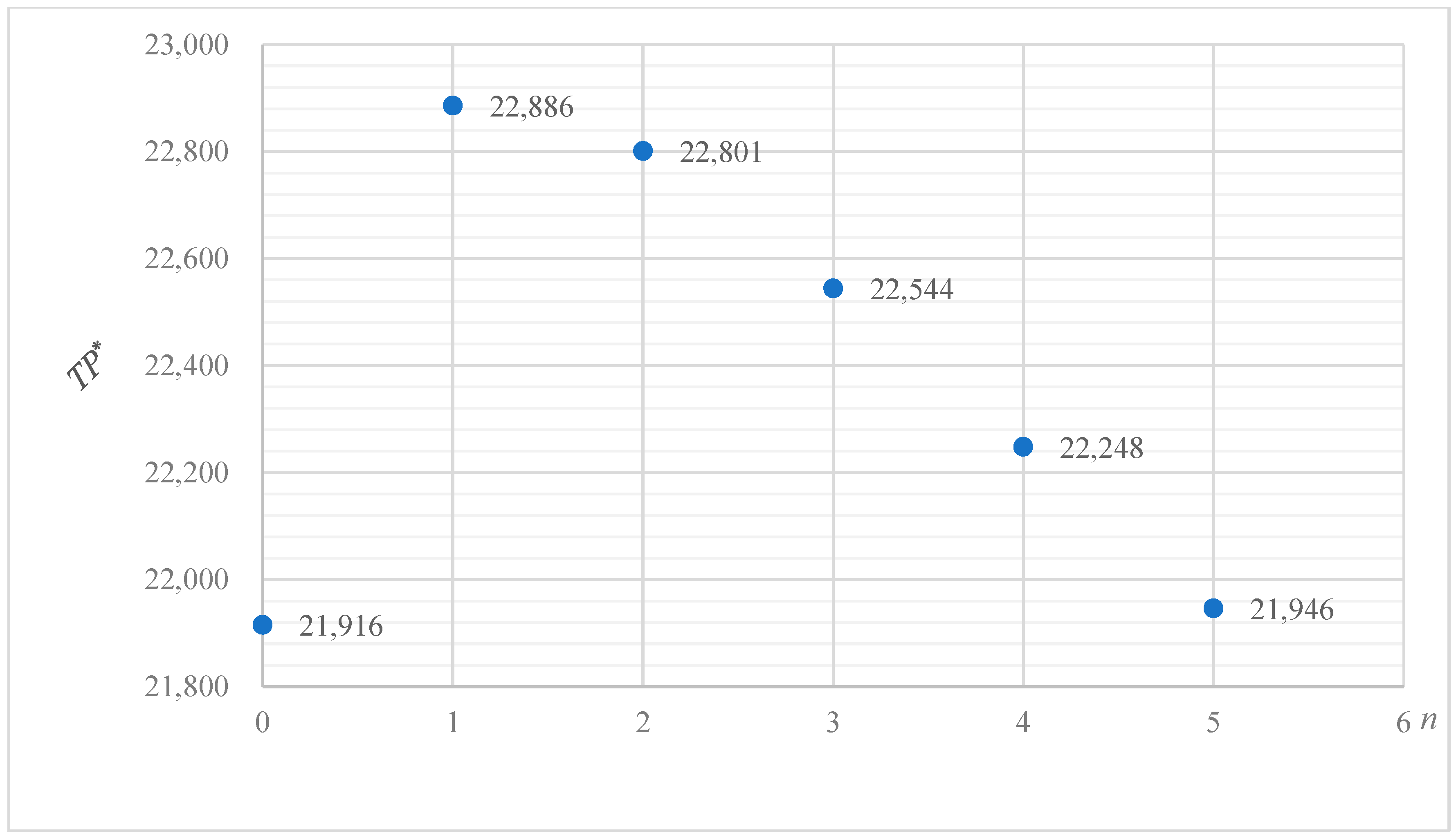
The empirical results, demonstrated by the proposed algorithm, calculate as follows: optimal maintenance checks $n^{\mathrm{*}}=$1; an optimal production cycle length of $t_1^{*}$ = 0.1675 months; an optimal replenishment cycle length of T^* = 0.5384 months; an optimal time interval between each maintenance check of ${t_a}^{*}$ = 0.0873 months; the total carbon emissions per month is $TE=$5030.6 kg; and the total profit per month is TWD 22,886. The entire solution process and optimal solution values are shown in

Table 3. Solving process of optimal solution.

$\mathit{n}$	${\mathit{t}}_1$	T	${\mathit{t}}_{\mathit{a}}$	$\mathit{T}\mathit{E}/\mathit{T}$	$\mathit{T}\mathit{P}$
0	0.1074	0.3304	0.1074	5166.4	21,916
1	0.1675 *	0.5384 *	0.0837 *	5030.6 *	22,886 *
2	0.2021	0.6586	0.0674	5029.2	22,801
3	0.2291	0.7514	0.0573	5052.1	22,544

Note: The symbol * represents the optimal solution for the proposed model.

. By comparing the scenario without maintenance (n = 0), it can be found that proper equipment maintenance not only contributes to the low-carbonization of manufacturing but can also effectively increase the total profit compared with no equipment maintenance. Furthermore, Figure 2 presents a graphical illustration of the total profit with respect to $t_1$ for n = 1, and Figure 3 displays an illustration of the optimal total profit versus n, which implies the concavity of the proposed model can be verified.

4.2. Sensitivity Analysis

In order to understand the impact of parameter changes on the optimal solutions, this study intends to conduct a sensitivity analysis of the parameters of the proposed model. By using the same values as the example in Table 2, the individual parameters are increased or decreased by 10% or 20%, while other parameters remain unchanged. Based on the changes in various parameters, the impact on the optimal decision variables, total amount of carbon emissions, and total profit are illustrated in Figure 4, Figure 5, Figure 6, Figure 7, Figure 8, Figure 9, Figure 10, Figure 11, Figure 12, Figure 13, Figure 14, Figure 15, Figure 16 and Figure 17 and also tabulated in

Table 4. Sensitivity analysis of parameter changes.

Parameter	Value	$\mathit{n}$	${\mathit{t}}_1$	T	${\mathit{t}}_{\mathit{a}}$	$\mathit{T}\mathit{E}/\mathit{T}$	$\mathit{T}\mathit{P}$
$P$	4000	2	0.3528	0.9159	0.1176	5062.0	23,766
	4500	2	0.2535	0.7425	0.0845	5034.9	23,195
	5000	1	0.1675	0.5384	0.0837	5030.6	22,886
	5500	1	0.1415	0.5011	0.0707	5029.2	22,656
	6000	1	0.1229	0.4754	0.0614	5029.6	22,474
$D$	1200	1	0.1292	0.5207	0.0646	4063.4	17,564
	1350	1	0.1468	0.5252	0.0734	4546.5	20,200
	1500	1	0.1675	0.5384	0.0837	5030.6	22,886
	1650	2	0.2357	0.6977	0.0786	5513.6	25,636
	1800	2	0.2818	0.7637	0.0939	6007.4	28,554
$a$	0.04	1	0.1655	0.5349	0.0828	5006.1	22,733
	0.045	1	0.1665	0.5366	0.0832	5018.3	22,809
	0.05	1	0.1675	0.5384	0.0837	5030.6	22,886
	0.055	1	0.1684	0.5401	0.0842	5043.0	22,963
	0.06	1	0.1695	0.5419	0.0847	5055.5	23,041
$b$	0.4	1	0.1572	0.5069	0.0786	5012.7	22,699
	0.45	1	0.1621	0.5218	0.0810	5021.2	22,791
	0.5	1	0.1675	0.5384	0.0837	5030.6	22,886
	0.55	1	0.1735	0.5570	0.0868	5041.3	22,985
	0.6	2	0.2211	0.7194	0.0737	5052.4	23,091
$S$	400	1	0.1572	0.5058	0.0786	5021.8	23,078
	450	1	0.1624	0.5223	0.0812	5026.1	22,980
	500	1	0.1675	0.5384	0.0837	5030.6	22,886
	550	1	0.1724	0.5540	0.0862	5035.2	22,794
	600	1	0.1772	0.5692	0.0886	5039.9	22,705
$v$	16	1	0.1576	0.5072	0.0788	5022.1	28,541
	18	1	0.1623	0.5220	0.0812	5026.1	25,712
	20	1	0.1675	0.5384	0.0837	5030.6	22,886
	22	1	0.1731	0.5565	0.0866	5036.0	20,063
	24	2	0.2203	0.7176	0.0734	5046.3	17,293
h	5	2	0.2464	0.8021	0.0821	5073.5	23,438
	4.5	1	0.1816	0.5834	0.0908	5044.4	23,131
	5	1	0.1675	0.5384	0.0837	5030.6	22,886
	5.5	1	0.1562	0.5025	0.0781	5020.9	22,659
	6	1	0.1469	0.4731	0.0735	5014.0	22,446
k	240	1	0.1614	0.5191	0.0807	5025.3	22,999
	270	1	0.1644	0.5288	0.0822	5027.9	22,942
	300	1	0.1675	0.5384	0.0837	5030.6	22,886
	330	1	0.1704	0.5478	0.0852	5033.4	22,831
	360	1	0.1733	0.5571	0.0867	5036.2	22,776
s	32	1	0.1675	0.5384	0.0837	5030.6	10,886
	36	1	0.1675	0.5384	0.0837	5030.6	16,886
	40	1	0.1675	0.5384	0.0837	5030.6	22,886
	44	1	0.1675	0.5384	0.0837	5030.6	28,886
	48	1	0.1675	0.5384	0.0837	5030.6	34,886
$\widehat{S}$	40	1	0.1665	0.5352	0.0832	5011.1	22,905
	45	1	0.1670	0.5368	0.0835	5020.9	22,895
	50	1	0.1675	0.5384	0.0837	5030.6	22,886
	55	1	0.1679	0.5400	0.0840	5040.4	22,877
	60	1	0.1684	0.5415	0.0842	5050.0	22,867
$\widehat{v}$	2.4	1	0.1680	0.5401	0.0840	4098.0	23,819
	2.7	1	0.1677	0.5393	0.0839	4564.3	23,353
	3	1	0.1675	0.5384	0.0837	5030.6	22,886
	3.3	1	0.1672	0.5375	0.0836	5496.9	22,419
	3.6	1	0.1669	0.5366	0.0835	5963.2	21,953
$\widehat{h}$	0.4	1	0.1700	0.5465	0.0850	4985.3	22,933
	0.45	1	0.1687	0.5424	0.0844	5008.1	22,910
	0.5	1	0.1675	0.5384	0.0837	5030.6	22,886
	0.55	1	0.1662	0.5344	0.0831	5052.9	22,863
	0.6	1	0.1650	0.5306	0.0825	5074.8	22,839
$\widehat{k}$	16	1	0.1671	0.5371	0.0835	5022.8	22,893
	18	1	0.1673	0.5377	0.0836	5026.7	22,890
	20	1	0.1675	0.5384	0.0837	5030.6	22,886
	22	1	0.1677	0.5390	0.0838	5034.5	22,882
	24	1	0.1679	0.5396	0.0839	5038.4	22,879
$u_b$	0.8	1	0.1692	0.5438	0.0846	5032.2	23,892
	0.9	1	0.1683	0.5411	0.0841	5031.4	23,389
	1	1	0.1675	0.5384	0.0837	5030.6	22,886
	1.1	1	0.1666	0.5358	0.0833	5029.9	22,383
	1.2	1	0.1658	0.5333	0.0829	5029.2	21,880

.

According to the results in Table 2, we can obtain the following meaningful findings:

• When the demand rate, defect rate parameter, or production cost increases to a certain threshold, or the production rate reduces or holding cost decreases to a certain threshold, the frequency of preventive maintenance will also increase;
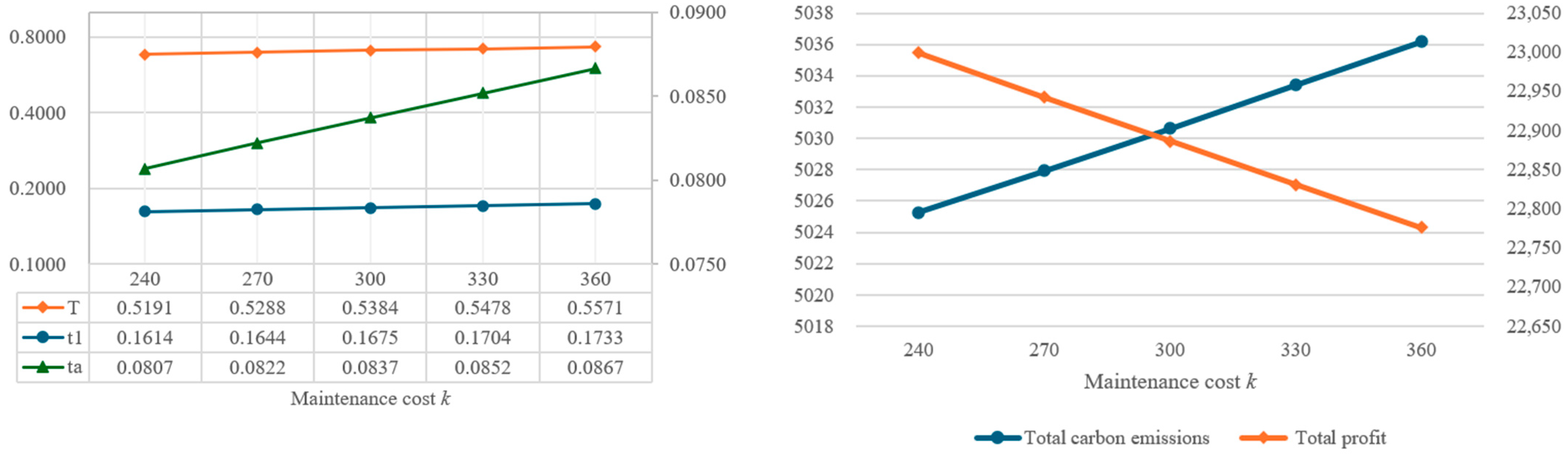
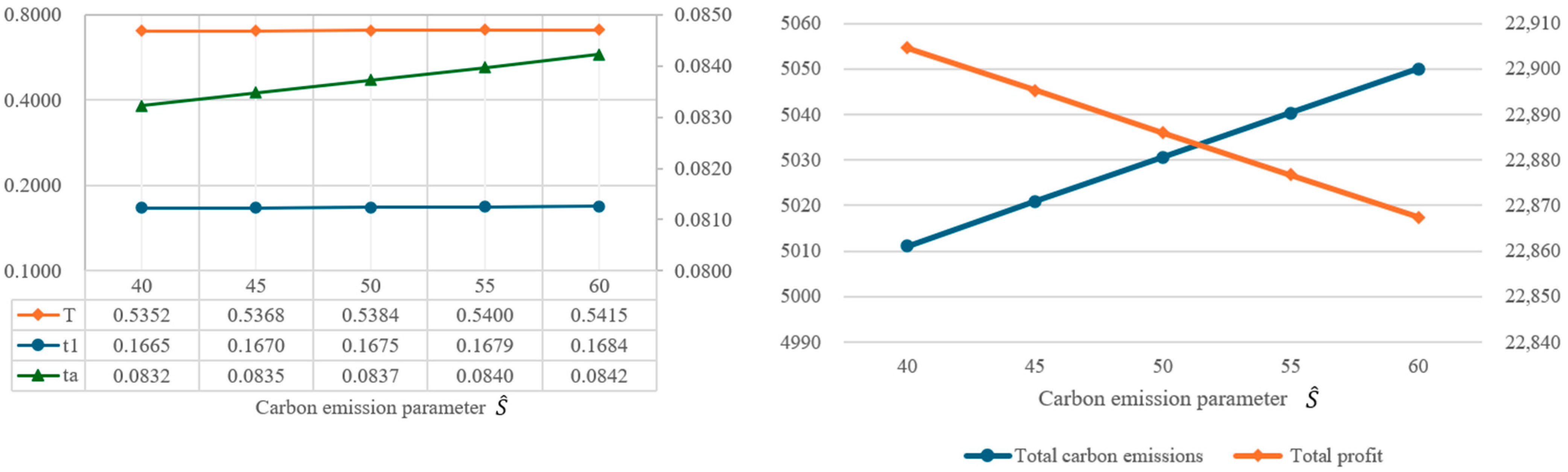
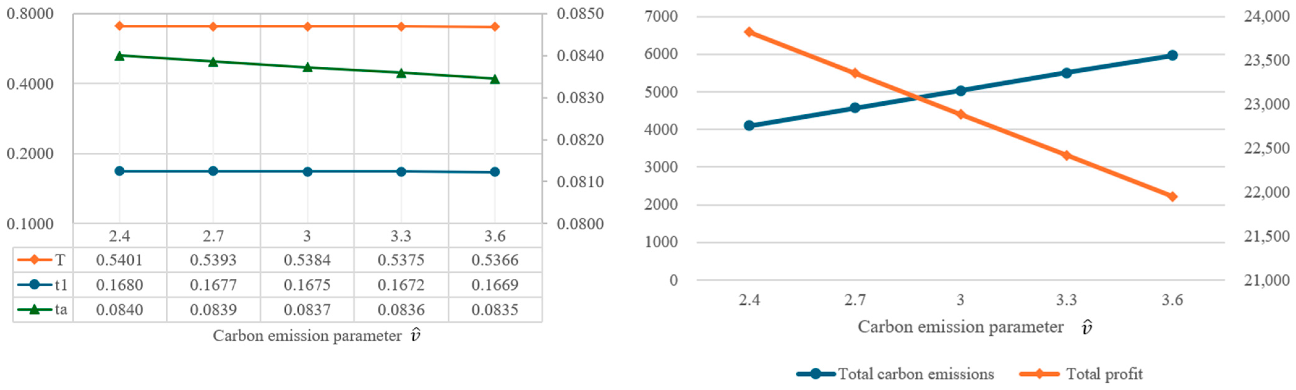
• With an increase in the fixed parameters occurring, such as setup cost, maintenance cost, carbon emissions generated by the set, or maintenance activity, this promotes optimal production cycle lengths and optimal intervals between each maintenance check. On the other hand, an increase in a variable parameter, such as the variable defect rate parameter, unit production cost, unit carbon emissions from product production, and unit carbon emissions from product storage, adversely impacts the optimal production cycle length and optimal intervals between each maintenance check;
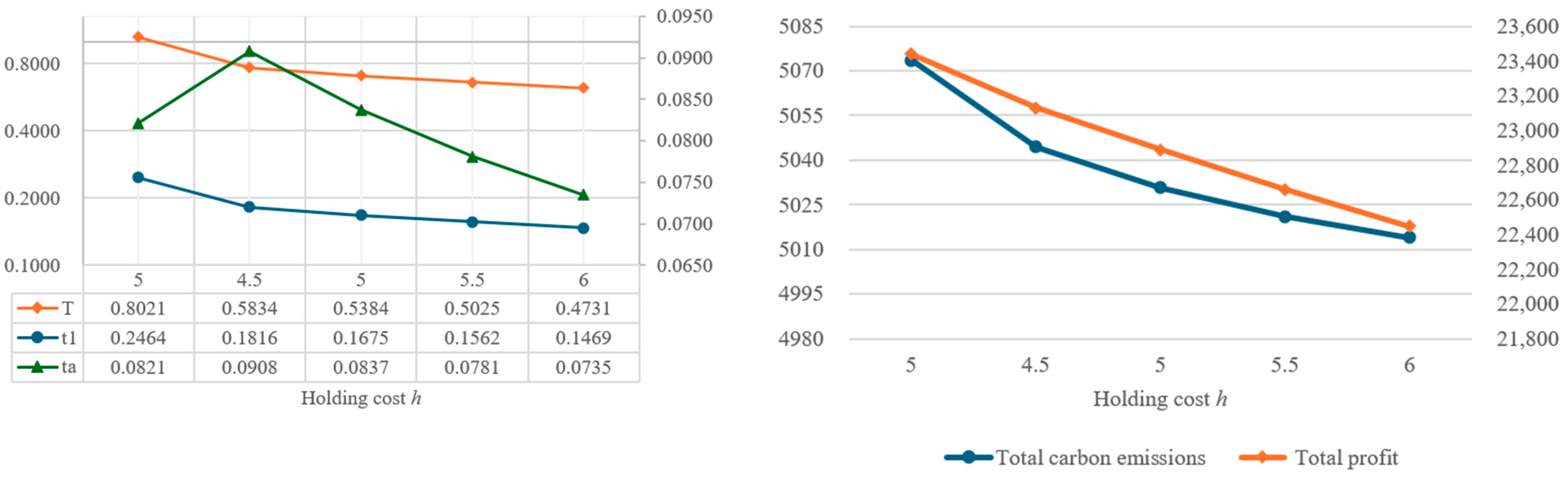
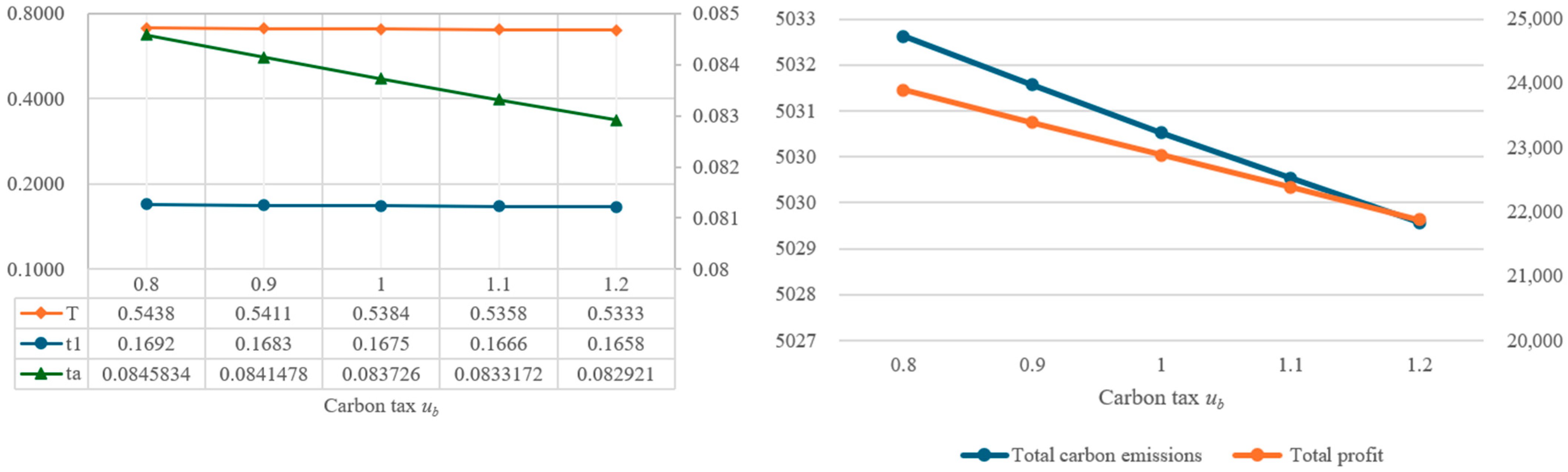
• Under the carbon tax policy, when the unit production cost and unit carbon tax increase, this will help reduce the amount of carbon emissions. Moreover, when the production rate increases, the amount of carbon emissions will first increase and then decrease; when the unit holding cost increases, the amount of carbon emissions will first decrease and then increase;
• As the unit holding cost increases, the length of the production cycle, the length of the maintenance cycle, and the amount of carbon emissions will decrease initially; however, once the number of maintenance checks decreases, the length of the production cycle, the length of the maintenance cycle, and the amount of carbon emissions will increase as the holding cost increases.

5. Discussion and Conclusions

Different from the previous research literature, this study simultaneously incorporated preventive maintenance and carbon emission issues into the economic production quantity model to explore how a manufacturer can determine the optimal production cycle length and preventive maintenance frequency under the carbon tax policy so that the total profit per unit time has a maximum value. In the numerical analysis, this study takes the disposable diaper manufacturer as an example. Based on the actual business situation of the manufacturer, a numerical example and parameter sensitivity analysis are conducted. Following, this study summarizes the research conclusions based on the numerical analysis results in the previous section, further explains the practical management implications, and finally derives feasible future research directions based on the limitations of this study.

5.1. Discussion

According to empirical results, the meaningful management insights are as follows:

• During the production process, timely maintenance can indeed help reduce carbon emissions and increase total profits. Especially when the demand rate, product defect rate, or setup cost increases to a certain threshold, the frequency of preventive maintenance will also increase;
• Fixed-cost parameters have a positive impact on the optimal production cycle length and optimal maintenance cycle length. That is, as the value of such parameters increases, both the optimal production cycle length and optimal maintenance cycle length increase. This effect is exactly opposite to the variable-cost or carbon-emission parameters.
• Under the trend of rising prices of global materials and the internalization of carbon-emission costs, the increase in the manufacturer’s unit production cost and unit carbon tax will prompt the manufacturer to reduce the amount of carbon emissions.
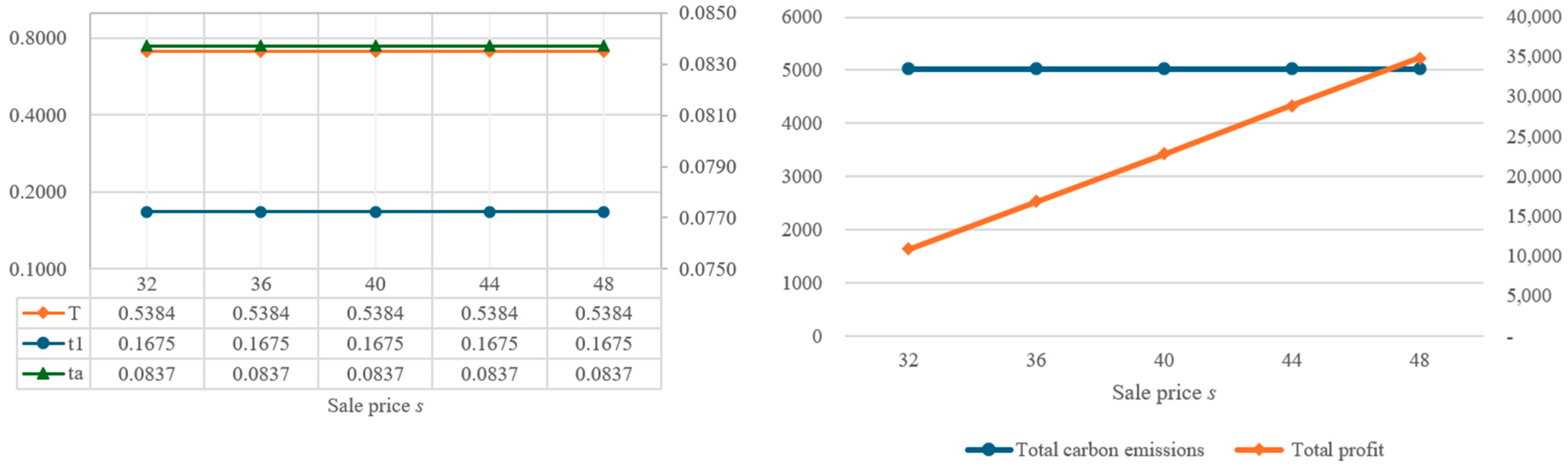
• The manufacturer’s total profit will increase as demand rates or sales prices increase; while increases in the production rate, fixed defect rate, variable defect rate, setup cost, production cost, holding cost, or maintenance cost will have a negative impact on total profit;
• When the time-varying defect rate is considered and maintenance checks are allowed, the manufacturer’s unit holding cost increases, and the production cycle length, maintenance cycle length, and carbon emissions will first decrease and then increase. That is, the unit holding cost is an important trade-off parameter for the manufacturer’s production cycle length and maintenance cycle length.

5.2. Management Revelations

In summary, under the carbon tax policy, it is essential for companies to make strategic adjustments in their equipment maintenance and inventory management. The results of this study show that by optimizing inventory levels and equipment maintenance frequency, companies can achieve maximum economic benefits under the burden of the carbon tax. Regarding the practical application of the proposed model, it may be possible to develop a small decision support system or directly embed it into an enterprise-related operation management system (such as an ERP system) to provide managers with a relatively objective reference before making relevant decisions. This not only helps reduce environmental impact but also improves the competitiveness and sustainable development of enterprises.

This research can be extended in several directions in the future. First, this study considers the constant demand rate while it may be related to price, inventory level, or low-carbon investment; hence, the variable demand rate is worth considering in the future. Another expansion direction can also include multi-agent decision-making behavior under carbon tax based on prospect theory and mental accounting [26]. Furthermore, there may be many types of goods sold by an enterprise, and the demand for each commodity may be different, so the production rate needs to be different. Therefore, the issue of the production–inventory model with multiple products is also worthy of discussion. In addition, the cost of each maintenance check in this model is fixed. In the future, different maintenance types and costs can be considered to be more consistent with actual scenarios. Lastly, this research can be extended by considering scenarios such as allowing shortages, trade credit, discounts on amounts, or other carbon-emission policies [27].

References

- Lok, Y.W.; Supadi, S.S.; Wong, K.B. EOQ Models for Imperfect Items under Time Varying Demand Rate. Processes 2022, 10, 1220. [Google Scholar] [CrossRef]
- Harris, F.W. How many parts to make at once. Mag. Manag. 1913, 10, 135–136. [Google Scholar] [CrossRef]
- Taft, E.W. The most economical production lot. Iron Age 1918, 101, 1410–1412. [Google Scholar]
- Porteus, E.L. Optimal lot sizing, process quality improvement and setup cost reduction. Oper. Res. 1986, 34, 137–144. [Google Scholar] [CrossRef]
- Salameh, M.K.; Jaber, M.Y. Economic production quantity model for items with imperfect quality. Int. J. Prod. Econ. 2000, 64, 59–64. [Google Scholar] [CrossRef]
- Chiu, Y.P. Determining the optimal lot size for the finite production model with random defective rate, the rework process, and backlogging. Eng. Optim. 2003, 35, 427–437. [Google Scholar] [CrossRef]
- Khan, M.; Jaber, M.Y.; Bonney, M. An economic order quantity (EOQ) for items with imperfect quality and inspection errors. Int. J. Prod. Econ. 2011, 133, 113–118. [Google Scholar] [CrossRef]
- Yuan-Shyi, C.P.; Chen, H.Y.; Chiu, W.S.; Chiu, V. Optimization of an economic production quantity-based system with random scrap and adjustable production rate. J. Appl. Eng. Sci. 2018, 16, 11–18. [Google Scholar] [CrossRef]
- Taleizadeh, A.A.; Soleymanfar, V.R.; Govindan, K. Sustainable economic production quantity models for inventory systems with shortage. J. Clean. Prod. 2018, 174, 1011–1020. [Google Scholar] [CrossRef]
- Daryanto, Y.; Wee, H.M. Sustainable economic production quantity models: An approach toward a cleaner production. J. Adv. Manag. Sci. 2018, 6, 206–212. [Google Scholar] [CrossRef]
- Daryanto, Y.; Wee, H.M. Low carbon economic production quantity model for imperfect quality deteriorating items. Int. J. Ind. Eng. Eng. Manag. 2019, 1, 1–8. [Google Scholar] [CrossRef]
- Sinha, S.; Modak, N.M. An EPQ model in the perspective of carbon emission reduction. Int. J. Math. Oper. Res. 2019, 14, 338–358. [Google Scholar] [CrossRef]
- Fadlil, I.N.; Novitasari, R.; Jauhari, W.A. Sustainable economic production quantity model with rework and product return policy. AIP Conf. Proc. 2020, 2217, 030078. [Google Scholar]
- Gharaei, A.; Almehdawe, E. Optimal sustainable order quantities for growing items. J. Clean. Prod. 2021, 307, 127216. [Google Scholar] [CrossRef]
- Karim, R.; Nakade, K. A literature review on the sustainable EPQ model, focusing on carbon emissions and product recycling. Logistics 2022, 6, 55. [Google Scholar] [CrossRef]
- Paul, A.; Pervin, M.; Pinto, R.V.; Roy, S.K.; Maculan, N.; Weber, G.W. Effects of multiple prepayments and green investment on an EPQ model. J. Ind. Manag. Optim. 2023, 19, 6688–6704. [Google Scholar] [CrossRef]
- Cassady, C.R.; Bowden, R.O.; Liew, L.; Pohl, E.A. Combining preventive maintenance and statistical process control: A preliminary investigation. IIE Trans. 2000, 32, 471–478. [Google Scholar] [CrossRef]
- Wang, H.Z. A survey of maintenance policies of deteriorating systems. Eur. J. Oper. Res. 2002, 139, 469–489. [Google Scholar] [CrossRef]
- Kim, D.; Lim, J.H.; Zuo, M.J. Optimal schedules of two periodic preventive maintenance policies and their comparison. In Engineering Asset Lifecycle Management, Proceedings of the 4th World Congress on Engineering Asset Management, Athens, Greece, 28–30 September 2009; Springer: London, UK, 2010; pp. 449–457. [Google Scholar]
- Schutz, J.; Rezg, N.; Léger, J.B. Periodic and sequential preventive maintenance policies over a finite planning horizon with a dynamic failure law. J. Intell. Manuf. 2011, 22, 523–532. [Google Scholar] [CrossRef]
- Lin, T.W.; Wang, C.H. A hybrid genetic algorithm to minimize the periodic preventive maintenance cost in a series-parallel system. J. Intell. Manuf. 2012, 23, 1225–1236. [Google Scholar] [CrossRef]
- Liu, X.; Wang, W.; Zhang, T.; Zhai, Q.; Peng, R. An integrated non-cyclical preventive maintenance and production planning model for a multi-product production system. In Proceedings of the 2015 IEEE International Conference on Industrial Engineering and Engineering Management (IEEM), Singapore, 6–9 December 2015. [Google Scholar]
- Mazidi, P.; Mian, D.; Sanz-Bobi, M.A. Simulation model based on reliability and maintenance of a component and their effect on cost. In Proceedings of the 2016 China International Conference on Electricity Distribution (CICED), Xi’an, China, 10–13 August 2016. [Google Scholar]
- Yang, L.; Zhao, Y.; Peng, R.; Ma, X. Opportunistic maintenance of production systems subject to random wait time and multiple control limits. J. Manuf. Syst. 2018, 47, 12–34. [Google Scholar] [CrossRef]
- Wu, T.; Ma, X.; Yang, L.; Zhao, Y. Proactive maintenance scheduling in consideration of imperfect repairs and production wait time. J. Manuf. Syst. 2019, 53, 183–194. [Google Scholar] [CrossRef]
- Deng, J.; Su, C.; Zhang, Z.M.; Wang, X.P.; Wang, C.P. Evolutionary game analysis of chemical enterprises’ emergency management investment decision under dynamic reward and punishment mechanism. J. Loss Prev. Process Ind. 2024, 87, 105230. [Google Scholar] [CrossRef]
- Mahato, F.; Mahato, C.; Mahata, G.C. Sustainable optimal production policies for an imperfect production system with trade credit under different carbon emission regulations. Environ. Dev. Sustain. 2023, 25, 10073–10099. [Google Scholar] [CrossRef]
Figure 1.
Relationship between inventory level and time within an imperfect production system.
Figure 2.
Illustration of the total profit with respect to for n = 1.
Figure 3.
The optimal total profit (TP*) under various values of n.
Figure 4.
Impact of changing P on the optimal solution.
Figure 5.
Impact of changing D on the optimal solution.
Figure 6.
Impact of changing a on the optimal solution.
Figure 7.
Impact of changing b on the optimal solution.
Figure 8.
Impact of changing S on the optimal solution.
Figure 9.
Impact of changing v on the optimal solution.
Figure 10.
Impact of changing h on the optimal solution.
Figure 11.
Impact of changing k on the optimal solution.
Figure 12.
Impact of changing s on the optimal solution.
Figure 13.
Impact of changing on the optimal solution.
Figure 14.
Figure 15.
Figure 16.
Figure 17.