Advancing Process Control in Fluidized Bed Biomass Gasification Using Model-Based Deep Reinforcement Learning

Abstract

This study presents a model-based deep reinforcement learning (MB-DRL) controller for the fluidized bed biomass gasification (FBG) process. The MB-DRL controller integrates a deep neural network (DNN) model and a reinforcement learning-based optimizer. The DNN model is trained with operational data from a pilot-scale FBG plant to approximate FBG process dynamics. The reinforcement learning-based optimizer employs a specially designed reward function, determining optimal control policies for FBG. Moreover, the controller includes an online learning component, ensuring periodic updates to the DNN model training. The performance of the controller is evaluated by testing its control accuracy for regulating synthetic gas composition, flow rate, and CO concentration in the FBG. The evaluation also includes a comparison with a model predictive controller. The results demonstrate the superior control performance of MB-DRL, surpassing MPC by over 15% in regulating synthetic gas composition and flow rate, with similar effectiveness observed in synthetic gas temperature control. Additionally, this study also includes systematic investigations into factors like DNN layer count and learning update intervals to provide insights for the practical implementation of the controller. The results, presenting a 50% reduction in control error with the addition of a single layer to the DNN model, highlight the significance of optimizing MB-DRL for effective implementation.

1. Introduction

As the world continues to seek cleaner and more sustainable sources of energy, biomass gasification is increasingly being recognized as one of the promising options for producing renewable energy [1,2]. This process involves converting solid biomass, such as wood chips or agricultural waste, into a synthetic gas that can be used as a fuel for power generation or other industrial processes. Several technologies have been developed for efficient biomass gasification at an industrial scale, such as fixed bed [3], entrained flow [4], and fluidized bed gasification [5]. Fluidized bed gasification (FBG) possesses a distinctive advantage by enabling the use of lump-form feedstock, notably pellets [6]. This feature proves advantageous for materials like biomass that pose challenges in grinding. Furthermore, FBG accommodates a variety of biomass feedstocks and enhances chemical reactions through efficient mixing and heat transfer [7,8]. Despite these merits, FBG’s industrial adoption remains limited. This is because achieving precise control over the FBG process to attain an optimal synthetic gas composition, flow rate, and temperature represents a formidable challenge with significant repercussions for process efficiency and sustainability [9]. For instance, suboptimal control of synthetic gas productivity, its composition, as well as its temperature can directly affect energy conversion, thereby diminishing the overall profitability of the gasification process [10]. Additionally, elevated levels of contaminants, like tar in synthetic gas, may induce corrosion and equipment fouling, and hinder downstream equipment efficiency [11,12]. To solve these problems, researchers have actively pursued optimal gas concentration using machine learning methods. Sezer et al. [13] developed an artificial neural network model to optimize synthetic gas exergy in an FBG. Similarly, Pandey et al. [14] showcased the potential of predicting synthetic gas composition through a comprehensive comparison of fundamental machine learning methods. These studies highlight the ability of machine learning models for efficient prediction in complex systems like FBG; however, further advancements are needed for industrial and commercial-scale modeling. The core challenge is limited data availability that can be addressed through the development of more advanced machine learning models [15].

While numerous studies have focused on modeling and optimizing synthetic gas [16,17,18], it is equally critical to emphasize the concurrent significance of developing an efficient control system for the FBG process. However, in the existing literature, only a limited number of studies have addressed this aspect [19,20,21]. Furthermore, the number of studies employing data or model-based controllers is even more limited [22,23]. However, recent advancements in machine learning methods have prompted efforts to explore machine learning-based controllers in biomass gasification. For instance, Wang et al. [24] developed a data-based predictive controller for biomass waste gasification in a supercritical water system, emphasizing its effectiveness in producing hydrogen-rich gas. Similarly, Karout et al. [25] explored a predictive controller for biomass gasification in a solar thermochemical reactor. While the efficiency of machine learning model-based controllers is a developing field, individual efforts are needed for specific applications, such as fluidized bed gasifiers, where dedicated studies are lacking [26].

In conventional practice, feedback control techniques such as proportional–integral–derivative (PID) controllers have been the preferred choice for regulating FBG. These PID controllers, even when they are carefully fine-tuned, often struggle with the intricate dynamics of FBG, particularly when faced with variations in biomass feedstock [27]. Model-based control strategies have emerged as a promising solution, relying on precise process models of biomass gasifiers to optimize performance and accommodate the inherent complexities of the FBG process. In recent studies [22,23], model-based control methods have been employed to regulate synthetic gas composition within gasifiers, albeit not exclusively in the context of FBG. These studies have utilized neural networks in the development of their model-based controllers. The selection of neural networks offers advantages owing to their ability to handle non-linear modeling and adapt to complex systems. However, it is essential to acknowledge that they often employ simpler neural network models, and as such, their generalization ability in real-time applications necessitates further assessment.

Moreover, they exhibit limitations such as the absence of real-time adaptability and online learning capabilities. These constraints emphasize the need for continued exploration and the development of advanced control strategies to enhance the effectiveness and adaptability of the controllers for intricate processes like FBG.

Another potential option is to develop a reinforcement learning-based controller. In recent years, there has been a growing interest in the use of reinforcement learning (RL), a type of machine learning, for process control. RL involves an agent learning to make decisions in an environment through trial and error, based on a reward function that indicates the success of its actions [28]. RL-based techniques have already shown great promise in various process control fields [29,30], including emergency control in power systems [31], autonomous voltage control [32], and traffic control in intelligent transportation systems [33]. Recent studies have also applied RL to control chemical processes like polymerization [34] and crystallization [35], as well as to biochemical processes [36]. However, the utilization of RL in FBG process control remains unexplored. This paper suggests that the intricate FBG control challenges, including the optimization of synthetic gas composition and temperature stability, can be reformulated as RL problems and addressed through the development of an advanced controller algorithm. Such a controller could facilitate RL-based learning, allowing for the acquisition of effective decision-making policies through trial and error. This integration of RL has the potential to significantly enhance the efficiency and sustainability of biomass gasification processes within the FBG context.

The present study aims to construct an advanced controller employing the RL for the FBG process. The implementation of RL is approached through a model-based RL method. This involves the utilization of a system model for the FBG process, allowing the controller to predict the consequences of its actions, resulting in a proactive control strategy. In contrast, the model-free RL method, which lacks a predictive model in its structure and relies solely on real-time interaction for learning [37], is considered less suitable for the FBG process due to its complex dynamics. Moreover, the controller is developed by synergistically integrating reinforcement learning and model predictive control (MPC) methods, capitalizing on their complementary predictive and control capabilities. Furthermore, a systematically designed deep neural network (DNN) functions as an information processor. The DNN learns the dynamics of the FBG process through the operational data derived from a pilot-scale FBG plant. The controller also incorporates an online learning element, facilitating continuous learning updates of the controller at predefined intervals. This dynamic adaptation mechanism ensures that both the DNN and the optimal control policy evolve together, effectively responding to real-time variations in FBG dynamics. Henceforth, the resultant controller is designated as a model-based deep reinforcement learning (MB-DRL) controller.

In this study, the DNN model is derived from our preceding work [38], where we systematically assessed various neural network types and architectures to predict process parameters in the FBG plant. Specifically, our prior study established the efficacy of LSTM and GRU for modeling the complex and dynamic behavior of the FBG, providing crucial insights into the most effective neural network approach. In this current study, we take a step forward, focusing on the development of the MB-DRL controller for the FBG. The primary objective is to address control challenges and create a responsive, adaptive controller for the FBG. However, the success of the MB-DRL is dependent on the accuracy and computational efficiency of the DNN model.

The paper’s structure is as follows: Section 2 discusses the background of the fluidized bed biomass gasification plant employed in our investigation, concurrently discussing the intricate process control challenges associated with it. Section 3 elaborates on the conceptualization and construction of the proposed controller as well as its method of implementation. Section 4 discusses the results of the proposed controller’s performance assessments. Finally, Section 5 summarizes the conclusions of the study and highlights the major findings.

2. Background

2.1. Biomass Gasification Plant

In this section, an overall description of the designated process system is presented. The system is a bubbling-type fluidized bed biomass gasification plant located at the Fraunhofer Institute for Factory Operation and Automation IFF in Magdeburg, Germany. The development of a model-based reinforcement learning controller is undertaken with this system as the target. For an in-depth comprehension of the operational intricacies, the reader’s attention is directed to Figure 1, which offers a depiction of the process flow as well as essential instrumentation and control within the aforementioned gasification plant.

The gasification plant is operated with a continuous biomass supply, utilizing wood chips with lengths ranging from 1 to 10 mm to generate synthetic gas. These chips consist of a blend of wood materials, including pine, larch, and spruce. The ultimate analysis of the biomass wood chips is presented comprehensively in

Table 1. The ultimate analysis of the wood pellets (biomass) used as fuel in the fluidized bed biomass gasification pilot plant.

Element	Mass Fraction
Carbon	0.5125
Hydrogen	0.0594
Oxygen	0.4281

.

Biomass wood chips are initially stored in a dedicated biomass bunker. Then, prior to their introduction into the gasification reactor, the biomass undergoes preprocessing steps to reduce and stabilize its moisture content. Following this, the biomass is continuously fed into the gasification reactor through a screw conveyor, with the flow rate being carefully regulated via an electrically actuated process valve. This preprocessing is to maintain an overall consistent composition of the biomass feedstock, with some operational fluctuations.

To facilitate continuous gasification, primary air is supplied through a pipe located at the bottom of the gasification reactor, which further distributes the air evenly through a perforated plate equipped with multiple nozzles. Additionally, four secondary air inlets, situated just above the fluidized bed region (approximately 1.9 m from the bottom), are circumferentially distributed at equal intervals. The total secondary airflow is distributed among the four inlets. Both primary and secondary air supplies are generated using individual compressors and are regulated using electrically actuated process control valves. Moreover, ash residue removal is conducted manually through the ash valve during periods of substantial accumulation.

The gasifier is equipped with fourteen thermocouples to monitor temperatures at different heights. Thermocouples T1 to T9, located at heights of 0.105 m, 0.405 m, and 0.715 m, collectively monitor bed temperatures. T10 to T13, situated at heights of 1.662 m and 2.612 m, focus on freeboard temperatures, while T14, positioned at the outlet duct, captures the synthetic gas temperature. This distributed arrangement facilitates a thorough evaluation of thermal dynamics. Moreover, at the gasifier outlet duct, a gas analyzer measures CO and O₂ concentrations, and a flow sensor quantifies the flow rate of the synthetic gas.

Process control in this gasification plant is executed through the conventional programmable logic controller (PLC), in conjunction with an array of instruments and control equipment. Real-time information, encompassing gasification temperature, synthetic gas heating value, synthetic gas flow, and ash flow, among other parameters, is accessible to the process operator. The operator utilizes this information and their practical knowledge to make necessary adjustments and maintain the process at its optimal state.

2.2. Control Challenges

The efficient control of the given fluidized bed biomass gasification (FBG) plant poses numerous process control challenges due to the dynamic and nonlinear characteristics inherent in the FBG process. These challenges include non-uniform bed temperatures, uneven fluidization, tar and ash buildup, hotspot formations, and non-uniform heat transfer. Each one has a direct impact on the product which is synthetic gas. Accurate control of the synthetic gas composition is crucial. This is particularly important because of environmental regulations and economic considerations for subsequent processes such as gas cleaning.

In the continuous operation of the FBG plant, the responsibility for promptly addressing these control challenges falls squarely on the operators in the control room. Their decision-making process relies on a trio of critical factors: real-time feedback from the FBG plant, an analysis of operational data, and their expertise. However, operators in this plant work with a limited set of control options. Their primary means of action involve adjusting the flow rates of biomass and air, as well as controlling their respective temperatures. Another aspect of control lies in the preprocessing stage of the plant, which involves moisture reduction and stabilization in the biomass. However, variations in constituent elements of the biomass such as carbon content disturb the process, leading to rapid temperature spikes within the fluidized bed. This, in turn, poses formidable control challenges for plant operators.

These complexities associated with process control in FBG constitute a significant obstacle to the technology’s scalability in industrial applications. Consequently, despite the FBG technology’s longstanding presence in the field, its extensive adoption within commercial and industrial domains continues to be constrained. While FBG excels in efficiently handling various biomass types and converting them into synthetic gas, the challenge at an industrial scale is not merely the conversion to synthetic gas but achieving its consistent composition with a constant heat content or temperature, especially when utilizing diverse biomass feedstocks.

3. Methodology

3.1. Reinforcement Learning

Reinforcement learning (RL)-based control methods are rooted in the foundational assumptions of the Markov decision process (MDP). The central objective of these methods is to learn an optimal policy by iteratively optimizing a pre-defined mechanism, facilitated through the RL agent’s interactions with its environment. Specifically, at any given instance denoted as $t$ the governing policy is enacted based on the presently observed state, referred to as $s_t$. It takes the action $a_t$, and then receives the reward $r_t$. This state, in the MDP, is presumed to be temporally independent and inherently rich in data, thereby supporting optimal decision-making irrespective of temporal considerations.

However, complex challenges encountered in industrial process control, including the given case of the fluidized bed biomass gasification (FBG) process, deviate from the simplistic MDP approach. The intricate complexity and nonlinear nature inherent to FBG are influenced by an array of factors including temperature, pressure, and biomass fuel composition. This study aims to control the synthetic gas characteristics using input variables like flow rates of fuel and air as well as their temperature and moisture content. The adjustments to these input variables by the controller exhibit varied propagation times within the gasifier system to finally impact the synthetic gas composition or its temperature. Hence, the controller must be equipped to utilize the historical aspects of the process to efficiently control the synthetic gas in the FBG. Addressing the challenge of RL’s diminished performance stemming from the absence of historical data utilization can be achieved through strategies like incorporating Deep Q-networks (DQN) in RL. DQNs feature a replay buffer where prior data, encompassing states, actions, rewards, and subsequent states, are stored. Alternatively, approaches such as state augmentation can be employed, involving the enhancement of the current state representation with historical information. Moreover, reward shaping is another avenue wherein the reward function considers historical performance or deviations, indirectly guiding the RL agent’s decision-making process based on past data.

3.2. Model-Based Deep Reinforcement Learning Controller

Distinct from the conventional RL algorithms, this work develops a model-based deep reinforcement learning controller (MB-DRL). The MB-DRL uses a deep neural network (DNN) structure as an information processor to estimate the system dynamics, which is updated in real time to enhance the control robustness. Built upon this DNN, a control framework similar to the model predictive control (MPC) method is employed to learn the optimal control policy. Such a design offers flexibility for online applications and provides this MB-DRL approach to handle faults like sensor inaccuracies, actuator anomalies, and variations in biomass feedstock composition in the biomass gasifier.

In Figure 2, the internal functioning of the MB-DRL controller and its practical integration with the FBG process model are illustrated. At each time step, the controller computes the desired control actions, representing adjustments to input variables. These actions are subsequently transmitted to the process model for execution, with the resulting output fed back to the controller to establish a continuous feedback loop essential for information exchange and control optimization. The controller operates through two key components: a DNN model for predicting future process states and an optimizer for calculating control actions. While this approach aligns with established principles of model predictive control, it is important to note that the optimizer is purposefully designed with a unique objective—to maximize cumulative rewards, thereby introducing elements of reinforcement learning into the control process. The calculation of rewards is facilitated by a dedicated reward function, as discussed in Section 3.1. This reward function utilizes feedback from the process model and supplies the computed rewards to the optimizer. The details of the formulated reward function as well as the DNN model are presented in Section 3.2.2 and Section 3.2.1, respectively. Moreover, the controller’s online learning component continuously stores input and output data from the process model, allowing for DNN model updates at defined intervals. The selection of an appropriate learning update interval significantly influences the overall performance of this controller, a topic discussed in detail in Section 4.4.

3.2.1. System Dynamics—DNN Model

In the devised model-based deep reinforcement learning (MB-DRL) controller, firstly, a DNN model is developed to effectively approximate the intricate dynamics inherent in the FBG process. A DNN, characterized by its distinctive configuration of input, hidden, and output layers interlinked through neurons and weights, serves as a foundational component of our approach. Specifically, in this work, a specialized form of neural architecture known as a recurrent neural network (RNN) is used. This choice is made due to the ability of RNNs to learn the sequences of actions and states where temporal relationships play a pivotal role. RNNs are equipped to capture such dependencies, making them particularly suitable for tasks wherein the order of actions is of significance.

To enable effective training, operational data sourced from the FBG plant, comprising 20,000 data points recorded at intervals of 5 s, are utilized. The dataset has been evenly divided into two halves, with 50% allocated for model training, and an equivalent 50% designated for rigorous testing, facilitating a comprehensive evaluation and generalization assessment. Additionally, data preprocessing involves the use of the z-score normalization method to appropriately scale the data. Moreover, the mean squared error (MSE) metric has been adopted as the key measure (loss function) to quantify the deviation between predicted and actual process variable values, providing insight into the accuracy of the controller’s predictions. The DNN model is trained using supervised learning, to minimize a specified loss function. For both training and validation loss calculations, MSE is used as the loss function. The MSE equation, denoted as:

$$\mathrm{MSE}=\frac{1}{n}{\sum }_{i=1}^n{(y_i-\widetilde{y_i})}^2$$

(1)

where $y_i$ represents the target value, and ${\tilde{y}}_i$ represents the corresponding predicted values by the DNN model. $n$ is the number of data points. During training, the DNN model minimizes the training loss by adjusting parameters, while validation loss assesses the model’s generalization to new data, evaluating its performance beyond the training set.

The training process is visualized through training and validation loss profiles (Figure 3). The hyperparameter selection process of the DNN involves a systematic examination of each hyperparameter, utilizing MSE as the evaluation criterion. Subsequently, the chosen hyperparameters are listed in

Table 2. Configuration of the optimal DNN model.

Network Type	RNN
Number of input layer units	7
Number of units in 1st LSTM layer	120
Number of units in 2nd LSTM layer	72
Number of output layer units	3
Number of epochs (learning cycles)	1000
Batch size	48
Activation function	tanh
Optimizer	Adagrad
Performance evaluation function	Mean squared error

.

3.2.2. Reward Function

By utilizing the DNN, which predicts future process states of the synthetic gas within the FBG, an optimal control strategy is determined. This strategy aims to maximize a cumulative reward function denoted as $R_t$ (see Equation (5)), which serves as a performance measure. $R_t$ effectively cumulates various individual reward functions (Equations (2)–(4)) related to synthetic gas composition, temperature, and flow rate, providing the RL-based controller with the feedback needed to refine its decision-making process and enhance overall system efficiency.

$$r_{1,t}=\left\{\begin{array}{c}if\left|{CO}_{actual}-{CO}_{setpoint}\right|\le {\epsilon }_{CO}\\ r_t={\alpha }_t+c\\ else:\\ r_t=-\beta {\left|{CO}_{actual}-{CO}_{setpoint}\right|}^2-{\alpha }_t\end{array}\right.$$

(2)

$$r_{2,t}=\left\{\begin{array}{c}if\left|T_{actual}-T_{setpoint}\right|\le {\epsilon }_T\\ r_t={\alpha }_t+c\\ else:\\ r_t=-\beta {\left|T_{actual}-T_{setpoint}\right|}^2-{\alpha }_t\end{array}\right.$$

(3)

$$r_{3,t}=\left\{\begin{array}{c}if\left|F_{actual}-F_{setpoint}\right|\le {\epsilon }_F\\ r_t={\alpha }_t+c\\ else:\\ r_t=-\beta {\left|F_{actual}-F_{setpoint}\right|}^2-{\alpha }_t\end{array}\right.$$

(4)

$$R_t=r_{1,t}+r_{2,t}+r_{3,t}$$

(5)

At every time step, the RL agent collects the reward $R_t$. In this function, $c,\alpha ,$ and $\beta$ are constants. The individual rewards associated with target variables—$CO$ concentration, synthetic gas temperature ($T$), and synthetic gas flow rate ($F$)—are denoted as $r_{1,t}$, $r_{2,t}$, and $r_{3,t}$, respectively. Additionally, $\epsilon$ denotes the permissible tolerance for deviation in the value of a target variable from its defined set point. In contrast to a reward solely based on the difference between the set points and actual values, a temporal component is also integrated into the reward function. Whether the output attains or misses the predetermined range, there is a time-weighted ${\alpha }_t$ term accounting for the temporal aspect. This component provides additional rewards as the FBG process advances towards its target, motivating the agent to converge to the target range quickly. Moreover, this term applies an increased penalty to any divergence from the target range, thereby reinforcing a focused approach toward the end goal.

Furthermore, if the output moves away from the target range, the penalty is shaped by the squared difference between the measured output and the target value, incorporating the tolerance values ${\epsilon }_{CO}$, ${\epsilon }_T$, and ${\epsilon }_F$ to define the permissible range for each output variable. The introduction of the squared term augments sensitivity to deviations, effectively addressing offsets and outliers. Following each epoch, the cumulative reward emerges as the summation of individual rewards of each target variable and also across the entire operational duration.

3.3. FBG Process Model for Proposed Controller’s Performance Validation

To enable a comprehensive assessment of the controller’s capabilities in a dynamic environment, it is essential to develop a separate process model for the FBG process. In this context, using a neural network-based process model is highly advantageous due to the availability of process data from the FBG pilot plant’s operations. Developing a precise physical model for this inherently complex and nonlinear process is a daunting task. In contrast, neural networks can efficiently capture intricate data relationships, making them a better choice when there is ample operational data of the FBG at hand [38]. Leveraging this extensive dataset enables the neural network to understand the finer details of the gasification process, expediting model development and providing an accurate representation of real-world gasification dynamics. Consequently, it emerges as the ideal approach for the rigorous testing and continual refinement of the MB-DRL controller’s performance.

For the development of the FBG process model, the gated recurrent unit (GRU), a special variant of recurrent neural network models, is employed. The GRU distinguishes itself from other neural networks in its unique internal architecture, characterized by two gates: the reset gate and the update gate [39]. These gates grant the GRU the inherent ability to regulate memory retention and information flow within the network, facilitating its learning and prediction of sequential data. For a detailed illustration of the GRU’s structure and information flow within a neural network at a specific time step, readers are referred to Figure 4.

The reset gate serves to control how much of the previous information should be retained or forgotten, allowing the network to adapt its memory as needed. On the other hand, the update gate determines the extent to which the new memory state should overwrite the existing memory, helping the network incorporate relevant information from the current input. This streamlined architecture positions the GRU as an efficient choice for handling various sequential data tasks, striking a balance between memory capacity and computational efficiency.

Indeed, employing the GRU to develop a process model for the FBG process in this context presents compelling reasons, as outlined earlier. However, it is essential to recognize the potential for bias when employing neural network models both within the controller (referred to as DNN) and as the process model. A critical aspect of our approach lies in the data utilization strategy. While the data are sourced from the same FBG plant, a distinct and robust practice has been employed: the use of entirely separate datasets for training the GRU and the DNN models. This approach mitigates the risk of bias stemming from shared data and ensures that each neural network adapts to different phases of the plant’s behavior. Consequently, this approach not only reinforces the model’s generalization capabilities but also ensures a comprehensive evaluation of the controller’s performance under various conditions. From a technical standpoint, this data separation strategy aligns with best practices in neural network modeling and stands as a reasonable approach to minimize bias in our modeling and control framework.

Hence, regarding the training of the GRU model, a separate dataset containing 21,000 data points from the FBG plant is used. This dataset encompasses various process variables, including input parameters such as biomass and primary and secondary air flow rates. Moreover, the dataset includes measurements of the temperature of the synthetic gas, its composition, and flow rate. The GRU is trained to predict three output variables: the composition of synthetic gas, focusing on the concentration of CO, the temperature of the synthetic gas and its flow rate, using the input variables as presented in Figure 5. For reference, the optimal hyperparameters for the GRU-based process models are also presented in

Table 3. Configuration of the optimal GRU-based process model of FBG.

Neural Network Type	GRU
Number of input layer units	7
Number of units in the 1st GRU layer	94
Number of units in the 2nd GRU layer	78
Number of output layer units	3
Number of epochs (learning cycles)	1200
Batch size	24
Activation function	tanh
Optimizer	Adagrad
Loss function	Mean squared error (MSE)

.

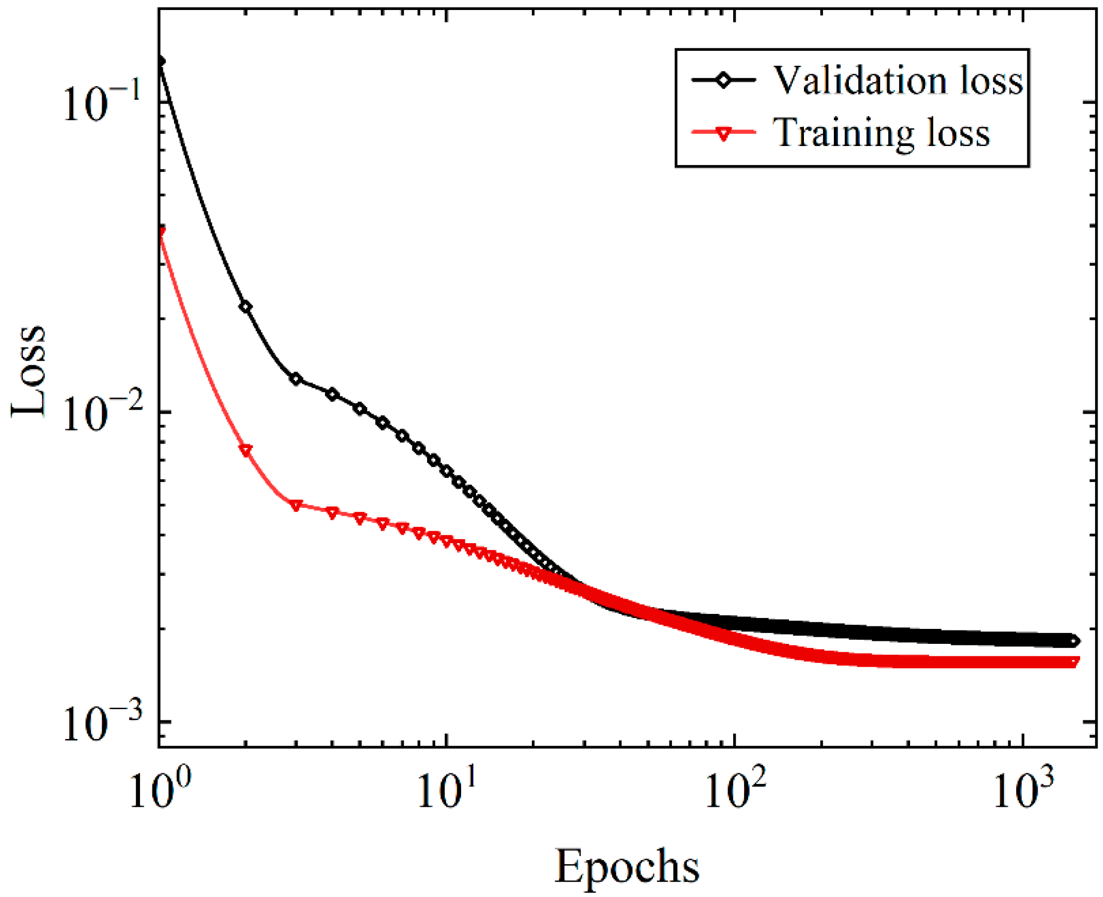
Throughout the training phase spanning 1200 epochs, the stability of both the training and validation errors is observed (see Figure 6). These errors, important for assessing the GRU model’s performance on respective datasets, consistently exhibited a stable trajectory. Importantly, this stability underscored the model’s capacity for generalization, reassuring us about the absence of overfitting or underfitting. Beyond training, the model’s predictive efficiency for each output parameter is evaluated using the unseen (validation) dataset, with results summarized in

Table 4. Performance summary of the gated recurrent unit-based process model of the fluidized bed biomass gasification process to predict values of output parameters.

Output Parameters	MAE [-]	RMSE [-]	Maximum MAE [-]
Synthetic gas temperature [°C]	8.59	11.9	29.64
Synthetic gas flow rate [m3/h]	0.63	0.71	2.14
Volumetric concentration of CO [%]	0.47	0.59	1.81

. In addition to the MSE metric used during training, the evaluation incorporated mean absolute error (MAE) and root mean squared error (RMSE), useful for understanding outlier sensitivity, interpretability, and precision.

4. Results and Discussion

This section evaluates the performance of the proposed model-based deep reinforcement learning (MB-DRL) controller for the FBG process. It includes evaluations of control performance, response time, the influence of the deep neural network (DNN) model depth on computational cost and control error, as well as the effects of adjusting the learning update interval. Additionally, a comparative analysis is conducted, benchmarking the performance of the MB-DRL controller against the well-established model predictive control (MPC) approach. The MPC also employs a pre-trained deep neural network (DNN) model for predicting future process states over a finite prediction horizon. Subsequently, the MPC optimizes control inputs, specifically manipulating the biomass fuel mass flow rate and primary and secondary air volumetric flow rates. The objective function, denoted as $J$ in Equation (6), operates as an objective function. It penalizes variations in input parameters and deviations from output temperatures. Minimizing $J$ at each sampling instant ensures optimal input values, guiding the MPC optimizer to maintain the values of the output parameters close to the desired setpoint.

$$J=\mathit{min}\{{\sum }_{t=1}^p{{(y}_t-y_{set})}^2+{\sum }_{t=1}^{c-1}({u_{i,t}-u_{i,t-1})}^2\}$$

(6)

Here, $p$ is the prediction horizon, $c$ is the control horizon, $y_t$ is the predicted value of the target parameter by the DNN model at time step $t$, $y_{set}$ is the set point, and $u_{i,t}$ is the control input at time $t$ in which subscripts $i$ represent the input parameters.

Moreover, the determination of the optimal prediction horizon for the MPC is established through a systematic analysis spanning prediction horizons from 15 to 90 s. For MPC, the best control accuracy is achieved while using the 50 s prediction horizon for all the target variables in the FBG process. Subsequently, an optimization framework is used to determine a required control sequence that adheres to constraints, within the FBG plant.

In comparison to MB-DRL, the key difference with MPC lies in how they compute optimal control actions for achieving desired process states or set points of the output parameters. Both controllers use a DNN model to predict future process states. However, in MPC, the optimizer determines the control action through iterative solutions of the objective function described in Equation (6). In contrast, the MB-DRL optimizer takes a different approach, iteratively calculating optimal control actions by considering the cumulative reward function outlined in Equations (2)–(5). This distinction in optimization methods reflects specific strategies employed by MPC and MB-DRL in achieving control objectives within the FBG system. Additionally, an advantage of MB-DRL is its online control, updating the DNN model after defined intervals.

4.1. Control Performance

The performance of the proposed controller (MB-DRL) is evaluated for three process variables, which are synthetic gas composition, temperature, and flow rate. For the synthetic gas composition, specifically achieving precise control over the required concentration of CO is tested. A dynamic reference trajectory is given for each of these process variables, and the controller is tasked to follow the desired trajectory while manipulating the input variables. This reference trajectory is acquired from the FBG plant operational data.

The implementation of the controller was executed in accordance with the presented graphical representation of the closed-loop system in Figure 2. Through 600 runs of closed-loop simulations, each referencing a time step of 5 s, the control test simulated the FBG process for a cumulative duration of 3000 s. Moreover, a learning update of the MB-DRL occurs after every 150 runs.

In the comparative evaluation with MPC, it is important to note that MPC lacks an online learning tool. To ensure a direct comparison, the MPC is assigned the same trajectory for each process variable, and the comparative assessment is visualized in Figure 7.

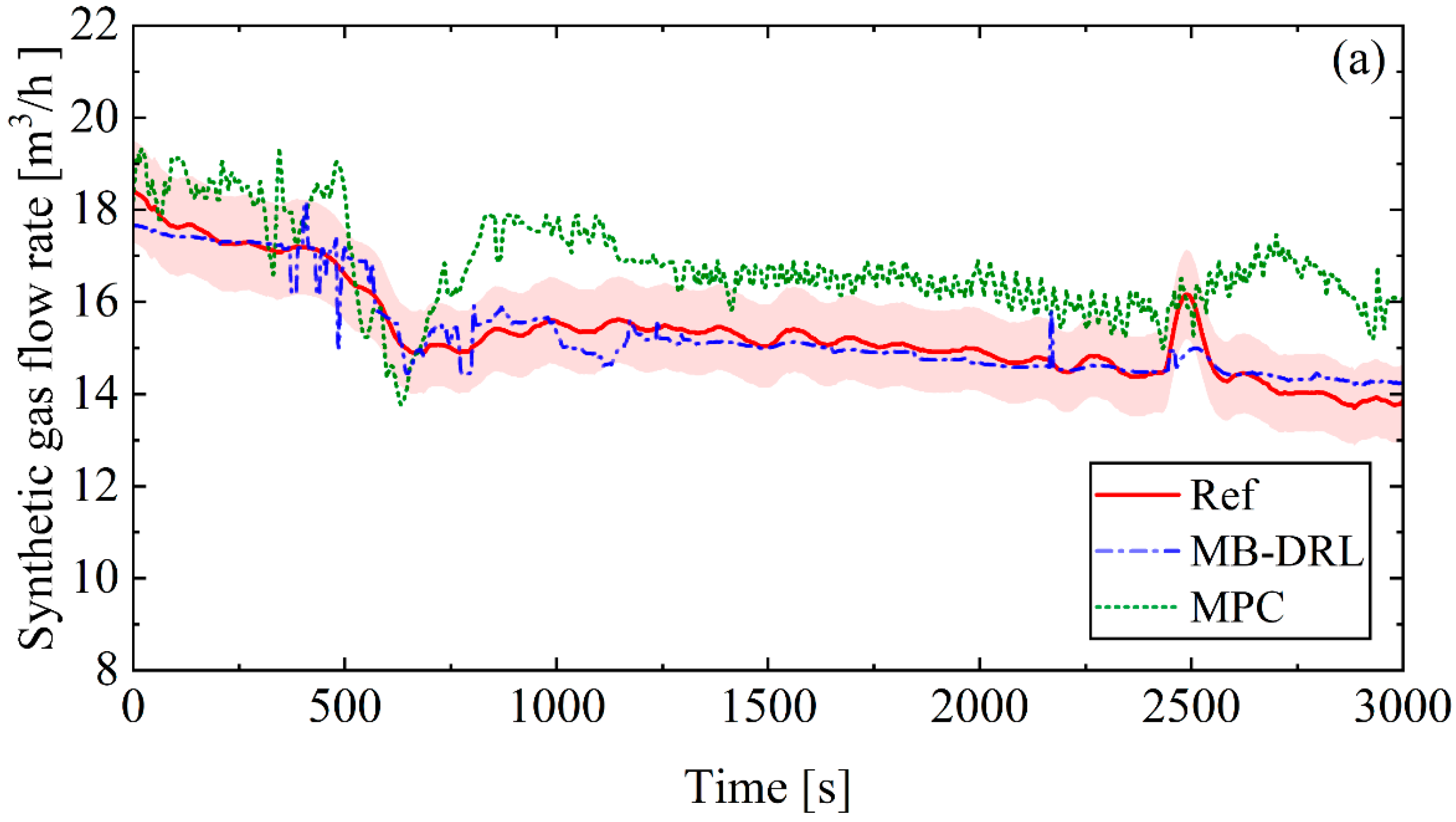
In Figure 7a, the effectiveness of the MB-DRL in regulating synthetic gas flow rate while ensuring stability and minimizing oscillations is evident. This differs from the performance of MPC, which encounters significant fluctuations during the initial phase and maintains this erratic behavior throughout the testing period. The proposed controller consistently showcases superior accuracy throughout the trial period, owing to its online learning component. This adaptive feature empowers the proposed controller to maintain stability even in the face of varying process dynamics.

Similarly, in Figure 7b, for controlling synthetic gas composition—specifically CO vol%—the MB-DRL effectively follows the reference trajectory, surpassing MPC’s performance. However, an anomaly is observed as the controller experiences a sudden decline (from 12 to 6 vol%) in CO at around 1200 s of the process simulation time. Upon repeated result realization to understand its cause, this anomaly consistently emerges once or twice, albeit at differing points. Moreover, across each iteration, the anomaly appears immediately following a learning update. Consequently, this behavior is linked to the DNN’s learning updates. However, it is important to underline that this behavior is not observed during the control performance tests of the MB-DRL for other variables. Despite this, the MB-DRL controller’s ability to closely adhere to the prescribed control trajectories highlights its promising efficacy.

Moving on to the analysis of temperature control in Figure 7c, both the MB-DRL and MPC demonstrate comparable performances, occasionally leaning in favor of MPC. This balance suggests that both approaches are suited to this specific control task (temperature control). The relatively improved performance of MPC is due to its effective learning of the FBG system dynamics to predict synthetic gas temperature accurately. The underlying DNN-based prediction mechanism in MB-DRL, along with its online learning component, has also maintained the synthetic gas temperature within the acceptable range.

Comparative insights between MB-DRL and MPC present their distinctive strengths and capabilities. MB-DRL has performed well in maintaining the values of the synthetic gas flow rate and its CO concentration to follow the reference trajectory. The control results present the MB-DRL’s capacity to learn and adapt. While the MPC, rooted in optimization, performs better at temperature control, predictive modeling has shown its dominant role. The dynamic nature of MB-DRL’s online learning component supports its efficiency against abrupt changes, while MPC’s stability is attributed to its optimization constraints.

4.2. Response Time

In the context of essential real-time applications for controlling the FBG process, the response time of the MB-DRL is a matter of critical significance, serving as an indicator of its efficiency and overall operability. The response time essentially refers to the computational time needed by the MB-DRL to calculate a control action at each time step. A comprehensive visualization of the response time for each run during the test (closed-loop simulation of 600 runs) of the MB-DRL to control the synthetic gas composition can be visualized in Figure 8. It should be emphasized that the assessment of response times excludes the overhead time associated with MB-DRL’s relearning or learning update, as that is proposed to be computed in parallel to the controlling tasks.

Overall, the response time of the MB-DRL maintains an acceptable level, averaging around 3 s. However, the MB-DRL displays a broader range of response times, indicating increased variability and unpredictability in its computational process. This phenomenon is particularly noticeable following learning updates that occur after every 150 runs (quantified as 750 s on the process time scale). While the observed changes in response time remain modest, staying below 5 s, they still hold significance. Moreover, this observation raises an interesting point: despite the consistent architecture of the MB-DRL’s DNN model in terms of its neuron count and layers, as well as the consistent input data shape and size, there exists a shift in the response time after each learning update.

The occurrence of these response time shifts during online training updates, coupled with their impact on adaptive control performance, introduces fluctuations that require consideration when scaling up this MB-DRL. This relationship between learning updates and the subsequent alterations in response time highlights the need for a comprehensive approach when extending the MB-DRL’s application to larger scales.

4.3. Impact of DNN Depth on Computational Cost and Control Error

As discussed in Section 4.2, the quicker response time of MB-DRL is critical for its application for real-time control of the FBG plant. The component of the MB-DRL which takes the most computational resources is its DNN model. Consequently, optimizing the DNN model during the MB-DRL construction is imperative to achieve control accuracy within the required response time. Specifically, the determination of optimal depth, indicating the number of layers in the DNN, and how it affects overall control performance is evaluated in this section.

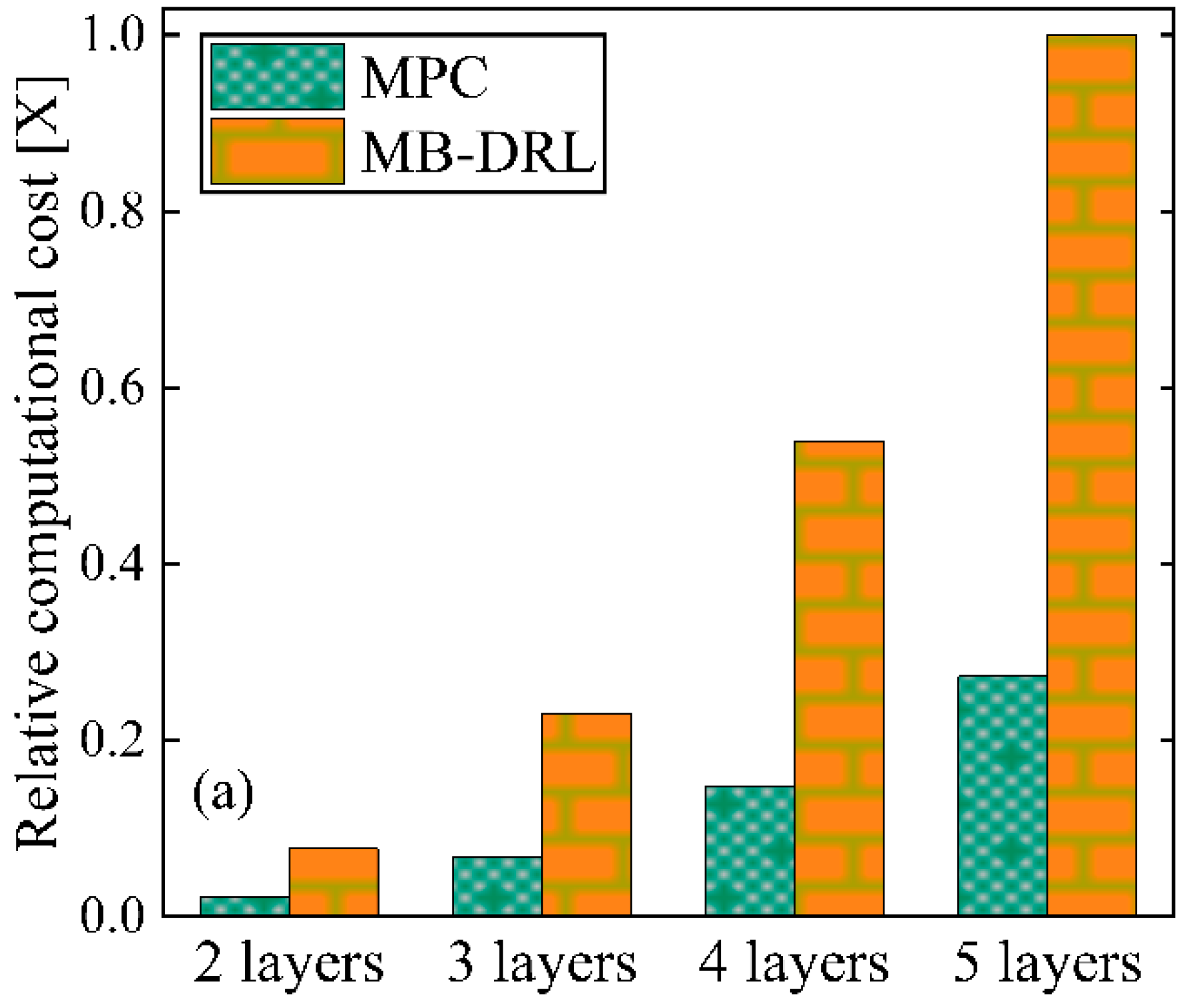
Figure 9a illustrates the trend of computational cost against the number of DNN layers, from two to five. As evident, increasing the depth of the DNN model within the MB-DRL leads to an exponential increase in computational cost. This observation aligns with the expected behavior, as deeper networks demand more computational resources for both forward and backward passes during training and inference. A comparative perspective is also established by comparing the computational cost of the MB-DRL against MPC, which remained consistently higher across all explored layer depths. In particular, when utilizing a five-layered DNN model, the computational cost of MB-DRL exceeds three times that of the computational cost of MPC with similar layer configurations. The increased computational cost of the MB-DRL is associated with its comprehensive design that includes the online learning component.

The evaluation further considered the consequences of changing the depth of the DNN on control error, a critical metric that reflects the performance of the control system. Figure 9b illustrates the control error values for both MB-DRL and MPC in which the MB-DRL outperformed MPC in terms of control error across all explored DNN depths. As the DNN depth increases, MB-DRL consistently exhibits reduced control error, indicating improved control performance. However, the error reduction is most significant, up to 50%, when transitioning from the second to the third layer. Beyond this point, the control error reduction becomes marginal with additional layers (four or five), accompanied by a substantial increase in computational cost. This suggests that a higher layer count is not a better choice. Moreover, although the control error profile hints at the three-layer DNN as optimal, our proposed MB-DRL with a two-layered DNN for FBG plant application prioritizes another crucial factor—response time. A three-layer DNN model does not meet the requirement of achieving an MB-DRL response time of less than 5 s.

These findings offer insights to practitioners seeking to optimize DNN architectures for real-time control applications. By comprehending the trade-offs between computational demands and control efficacy, engineers can make informed decisions regarding the design and deployment of DNN-based control systems.

4.4. Effect of Learning Update Interval on Control Performance and Computational Cost

The integral online learning update of MB-DRL significantly contributes to its overall performance, influencing both reliability and control accuracy. Following each set of 150 runs (defined as the learning update interval) in the closed-loop simulation, the controller’s DNN model is updated. This update is facilitated by integrating feedback data derived from the application of the controller to the process model. This dynamic learning mechanism enhances the MB-DRL controller’s adaptability and ensures continuous improvement over successive operational iterations. The selection of learning update intervals distinctly influences the equilibrium between control accuracy and computational resource utilization. To evaluate this, a series of tests are conducted, encompassing learning update intervals spanning from 50 to 400 runs. The impact of these intervals on the MB-DRL performance is examined through two key metrics: control performance, quantified as mean absolute percentage error (MAPE), and computational cost. The outcomes of these examinations are presented in Figure 10, where the control error profile is presented by the red line, while the blue line represents the associated computational cost.

The analysis of computational costs in relation to learning update intervals reveals an expected but non-linear decline as the learning update interval increases. Simultaneously, the evaluation of the control error curve demonstrates a lack of a linear correlation with the learning update interval. In the initial phase, a shorter update interval (e.g., 100 runs) corresponds to a reduced control error, attributed to the rapid adaptation of the controller for precise trajectory tracking. Conversely, as the update intervals lengthen, the control error follows a more varied path.

The findings of these results provide the selection of an optimal learning update interval of the controller for the FBG process, specifically, 150 runs. The adoption of this interval not only results in reduced control error but also achieves a balance between control accuracy and computational efficiency, which holds significant implications for practical implementation. The established criterion in this study for computational efficiency is the attainment of a response time of less than 5 s by the controller.

This test presents the importance of conducting a thorough evaluation of control error during the application of the MB-DRL controller to identify the optimal learning update interval. Failure to optimize this interval not only compromises the efficiency of the controller but also renders it impractical for real-world applications. This emphasizes the need for an understanding of the intricate interplay between computational costs, learning update intervals, and control error for the effective deployment of the MB-DRL controller in FBG plants at an industrial scale.

4.5. MB-DRL Controller Limitations

While this study highlights the progress achieved with MB-DRL in controlling FBG, it is imperative to acknowledge specific limitations. The accuracy of the controller depends directly on the quality and representativeness of the training data. Although the online learning component of MB-DRL has demonstrated adaptability to these challenges, a significant shift in biomass composition can surpass the control capabilities of MB-DRL. Additionally, this study, which primarily centers on a pilot-scale FBG plant, prompts careful consideration when extrapolating the controller’s applicability to full-scale industrial operations, given potential dynamic complexities and geometric variations not fully accounted for in the DNN model parameters. Furthermore, the controller’s sensitivity to external disturbances or uncertainties, including faults, pump failures, line blockages, and safety concerns, requires further development, as the current MB-DRL configuration lacks specific provisions to handle such conditions.

5. Conclusions

In this study, a deep reinforcement learning-based controller is presented for real-time control in fluidized bed gasification (FBG) processes, with a primary focus on regulating synthetic gas properties such as composition, flow rate, and temperature. The controller incorporates a deep neural network for predictive modeling, a reinforcement learning framework for optimal control actions, and a continuous learning update component to adapt to new process conditions.

To evaluate the controller’s performance, we conducted a systematic analysis, comparing it with the conventional model predictive control (MPC) framework. The proposed controller demonstrates superior control accuracy, achieving over 15% improvement for both synthetic gas composition and flow rate. It also showed comparable performance in synthetic gas temperature control when compared to MPC. Notably, the controller consistently achieved a quick response time (<5 s) in all evaluations, highlighting its efficacy in real-time applications.

Furthermore, we also evaluated the computational challenges associated with implementing the controller, specifically analyzing the influence of deep neural network (DNN) depth on computational costs and control performance. Our findings indicate that a modest increase in DNN layers, specifically transitioning from two to three layers, can reduce control error by 50%, albeit with a three-fold increase in computational cost. Therefore, a careful tradeoff must be established between controller accuracy and response time in practical implementation.

In the continuation of this work, future research efforts will prioritize the integration of safety and economic constraints within the controller framework to ensure the secure operation of FBG while maximizing synthetic gas production efficiency.