Low Energy Cost Synchronization Strategy for Markovian Switching Complex Systems/Networks: Multiple Perspectives Comparative Analysis

Abstract

In this paper, the low energy cost synchronization control strategy of Markovian switching complex systems/networks is mainly studied and analyzed through multiple perspectives. Firstly, in order to achieve synchronization of Markovian switching complex networks with low energy cost, a control scheme based on the optimal node selection strategy that does not depend on the network coupling strength is improved, and a finite-time controller with a simpler structure is constructed. Secondly, based on the event-triggered control strategy an effective trigger event is designed to achieve the low energy cost synchronization of Markovian switching complex networks on the basis of reducing the information transmission and interaction between networks. Finally, the two control strategies mentioned in this paper are compared and analyzed from multiple perspectives through numerical simulations to better guide practical engineering.

1. Introduction

Complex systems and networks have received increasing recognition as an important tool for portraying and understanding real systems, especially in various fields such as biology, social systems, and engineering technology. Real systems often suffer from unexpected situations during operation, such as sudden changes in the environment, connection failure of the system, and system failure or maintenance, etc. [1,2,3]. These unexpected situations may cause the network topology to be re-linked, and thus the network operation state will be changed. The Markovian switching process can accurately describe such system/network topology switching process, and the system/network can be switched from one mode to another by Markov Process, which also coincides with the topology changes of the system/network [4,5,6]. Therefore, the complex network model with Markovian switching process gradually attracts the attention of many scholars and becomes a hot topic of current research.

Synchronization is an important class of clustering phenomena among the many dynamical behaviors of Markovian switching complex networks and has received more attention [7]. With the increasing standard of practical engineering requirements, the synchronization performance of the network is no longer the only criterion to measure network synchronization, as low control cost and low energy loss have become another concern of practical engineering. The commonly used control strategies are pinning control [8], linear (nonlinear) feedback control [9], adaptive control [10], intermittent control [11], impulse control [12], event-triggered control [13], etc. The characteristics of low energy consumption and low control cost of pinning control and event-triggered control have attracted the attention of many scholars. This paper will analyze the low-energy synchronous control problem of Markovian switching complex networks from multiple perspectives (optimal node selection strategy and event-triggered control strategy), to provide some theoretical basis for practical engineering.

It is well known that the pinning control strategy mainly reduces the control cost of the network on the basis of achieving synchronization by controlling a small number of nodes. However, how to select the control nodes of the network has been the focus of pinning control strategy research. In order to achieve the synchronization of the proposed multi-weight network model, an effective pinning controller was proposed in Ref. [14]. Same as Ref. [14], Ref. [15] only aims to achieve the synchronization behavior of the network by designing an effective and reliable pinning controller, but the importance of network pinning nodes selection is ignored. The problem of controlled node selection for pinning control strategy has been considered in Refs. [16,17,18], and the authors have proposed effective controlled node selection schemes while using pinning control strategies. However, during the Markovian switching complex network synchronization process, the performance metrics of each node in the network are dynamically changing, and how to track and exert control over these important nodes at each moment must also be considered. Moreover, the event-triggered control strategy reduces the information transmission and interaction between networks mainly through the designed trigger function, thus reducing the cost and energy loss of network control while achieving network synchronization [19,20]. Therefore, this paper will establish a node performance measure to track and control the important nodes at each moment, thereby achieving network synchronization with low energy consumption and low control cost, and better guide practical engineering.

Based on the above discussion, this paper mainly analyzes the pinning control (optimal node selection strategy) and event-triggered control strategy through multiple perspectives, and studies how to synchronize the network with low energy cost and low control cost, so as to better provide a theoretical basis for practical engineering. To the best of the knowledge of the authors, there are few studies on the node selection problem of pining control strategy, and there is currently no comparative study on optimal node selection strategy and event-triggered control strategy. Therefore, this research has certain theoretical and practical value.

This paper aims to achieve Markovian Switching complex network synchronization under low energy control cost and gives the basis for using the optimal node selection strategy and event-triggered control strategy under different actual conditions. For weakly coupling strength medium scale networks, the optimal node selection strategy can control less nodes to achieve faster low energy cost synchronization. For large scale networks with strong coupling strength, the event-triggered control strategy can achieve low energy cost synchronization faster, but requires slightly more nodes to be controlled than the optimal node selection strategy.

The rest of this paper is organized as follows. Some necessary formulas and mathematical models of network are given in Section 2. In Section 3, the control scheme based on the optimal node selection strategy is improved, and a controller with a simpler structure is constructed to achieve network synchronization with low control cost and low energy consumption. The theoretical proof of finite-time synchronization is given via the event-triggered control strategy in Section 4. In Section 5, the advantages and disadvantages of the two control methods are discussed through numerical simulations, and some conclusions are drawn for practical engineering purposes. Finally, Section 6 concludes the paper.

2. Network Models and Mathematical Preliminaries

In this section, some necessary assumptions and lemmas are given to complete the theoretical proof of Section 3 and Section 4.

We define a right-continuous Markovian process {r(t), t ≥ 0} in the complete probability space (Ω, F, {F_t}_t≥0, P), which takes values in the finite state space C = {1, 2, …, m} with generator Π = (π_pq)_m×m(p, q∈C). Define the transition probability (from the p-th mode at time t to the q-th mode at time t + ∆t) in the following form:

$$P\{r(t+\Delta t=q|r(t)=p\}=\{\begin{array}{cc}{\pi }_{pq}\Delta t+o(\Delta t)& ifq\ne p\\ 1+{\pi }_{pq}\Delta t+o(\Delta t)& ifq=p\end{array}$$

(1)

where $\begin{array}{c}\underset{\mathsf{\Delta }t\to 0}{\lim }\frac{o(\mathsf{\Delta }t)}{\mathsf{\Delta }t}=0(\mathsf{\Delta }t>0)\end{array}$, and π_pq ≥ 0 is the transition rate that satisfies:

$${\pi }_{pp}=-{\displaystyle \sum _{q=1,q\ne p}^m{\pi }_{pq}}$$

(2)

Consider a multiple weights Markovian switching complex dynamical network composed of N nodes with stochastic perturbations, in which each node is an n-dimensional dynamical system.

$$\begin{array}{ll}{\dot{x}}_i(t)=& f(t,x_i(t))+c_1{\displaystyle \sum _{j=1}^N{a}_{ij}(r(t)){\mathsf{\Gamma }}_1{x}_j(t)}+c_2{\displaystyle \sum _{j=1}^N{b}_{ij}(r(t)){\mathsf{\Gamma }}_2{x}_j(t)}\\ & +{\sigma }_i(t,x_i(t),r(t))\dot{\omega }(t),i=1,2,\dots ,N.\end{array}$$

(3)

where x_i(t) = (x_i1(t), x_i2(t), …, x_in(t))^T ∈ Rⁿ is the state vector of node i; f: Rⁿ→Rⁿ is a nonlinear vector function on x(t); c₁, c₂ > 0 denote the coupling strength of the network. Here, Γ₁ ∈ R^n×n and Γ₂ ∈ R^n×n are inner coupling matrices. A(r(t)) = (a_ij(r(t)))^N×N ∈ R^N×N and B(r(t)) = (b_ij(r(t)))^N×N ∈ R^N×N are the matrices representing the topological structure of the network at time t of mode r(t). $\begin{array}{c}\omega (t)={\left({\omega }_1(t),{\omega }_2(t),\dots ,{\omega }_n(t)\right)}^T\end{array}$ is an n-dimensional Brown motion; $\begin{array}{c}{\sigma }_i(t,x_i(t),r(t))\end{array}$ is the noisy intensity function, mainly used to describe the interference brought by the actual environment to the system.

The uncoupled node of the network (3) is given by:

$$\begin{array}{c}\dot{s}(t)=f(t,s(t))\end{array}$$

(4)

Here, the uncoupled node s(t) can be regarded as an isolated node system of the network (3).

Then, some lemmas and assumptions are given as follow.

Lemma 1

[21]. Assume that b₁, b₂, …, b_n are positive numbers, and c (0 < c < 1) is a positive constant. Then the following inequality holds

$${\left(b_1+b_2+\dots +b_n\right)}^c\le b_1^c+b_2^c+\cdots +b_n^c$$

(5)

Assumption 1.

There exists a non-negative constant ν and a symmetric positive matrix P, for $\forall x(t),y(t)\in R^n$, the nonlinear function f(·) satisfies

$$\begin{array}{c}{(x(t)-y(t))}^T(f(t,x(t))-f(t,x(t)))\le {(x(t)-y(t))}^T\nu P(x(t)-y(t))\end{array}$$

(6)

Assumption 2.

There exists a non-negative constant ρ_i, and the noise intensity function ${\sigma }_i\left(t,e_i(t),r(t)\right)$ satisfies the uniform Lipschitz condition, such that

$$trace\left[{\sigma }_i^T\left(t,e_i(t),r(t)\right){\sigma }_i\left(t,e_i(t),r(t)\right)\right]\le {\rho }_i(r(t))e_i^T(t)e_i(t)$$

(7)

3. Finite-Time Synchronization of Markovian Switching Complex Networks with Low Control Cost and Low Energy Consumption Based on Optimal Nodes Control Strategy

Based on the optimal node control strategy proposed in the previous research of the authors [22], combined with the Markovian switching complex network characteristics, sorting according to the node importance measurement indicators at different time intervals, some important nodes (nodes with greater impact on system synchronization) are selected as controlled nodes, and we then establish network models at different time intervals and design a controller with a simpler structure to achieve synchronization with low control cost and low energy consumption.

The Markovian switching complex network model based on the optimal node selection strategy in the time interval (t_k−1, t_k] can be written as

$$\{\begin{array}{ll}{\dot{x}}_i^k(t)=& f(t,x_i^k(t))+c_1{\displaystyle \sum _{j=1}^N{a}_{ij}(r(t)){\mathsf{\Gamma }}_1{x}_j^k(t)}+c_2{\displaystyle \sum _{j=1}^N{b}_{ij}(r(t)){\mathsf{\Gamma }}_2{x}_j^k(t)}\\ & +{\sigma }_i^k(t,x_i^k(t),r(t))\dot{\omega }(t)+u_i^k(t),i=o_{\max }^k(1),o_{\max }^k(2),\dots ,o_{\max }^{\delta }(l^k)\\ {\dot{x}}_i^k(t)=& f(t,x_i^k(t))+c_1{\displaystyle \sum _{j=1}^N{a}_{ij}(r(t)){\mathsf{\Gamma }}_1{x}_j^k(t)}+c_2{\displaystyle \sum _{j=1}^N{b}_{ij}(r(t)){\mathsf{\Gamma }}_2{x}_j^k(t)}\\ & +{\sigma }_i^k(t,x_i^k(t),r(t))\dot{\omega }(t),other\end{array}$$

(8)

where $\begin{array}{c}{o}_{\max }^k(\iota ),\iota =1,2,\dots ,l^k\end{array}$ denote the number of control nodes; $x_i^k(t)$ and $u_i^k(t)$ are the state variables and controller at time t_k.

According to Equations (4) and (8), the state error equation of the i-th node in network at time t_k is described as

$$\begin{array}{c}{e}_i^k(t)=x_i^k(t)-s(t),i=1,2,\dots ,N.\end{array}$$

(9)

We then bring (9) into (8), and the synchronization error dynamics system in the time interval (t_k−1, t_k] can be obtained

$$\{\begin{array}{ll}{\dot{e}}_i^k(t)=& f(t,x_i^k(t))-f(t,s(t))+c_1{\displaystyle \sum _{j=1}^N{a}_{ij}(r(t)){\mathsf{\Gamma }}_1{e}_j^k}+c_2{\displaystyle \sum _{j=1}^N{b}_{ij}(r(t)){\mathsf{\Gamma }}_2{e}_j^k}\\ & +{\sigma }_i^k(t,e_i^k(t),r(t))\dot{\omega }(t)+u_i^k,i=o_{\max }^k(1),o_{\max }^k(2),\dots ,o_{\max }^k(l^k)\\ {\dot{e}}_i^k(t)=& f(t,x_i^k(t))-f(t,s(t))+c_1{\displaystyle \sum _{j=1}^N{a}_{ij}(r(t)){\mathsf{\Gamma }}_1{e}_j^k}+c_2{\displaystyle \sum _{j=1}^N{b}_{ij}(r(t)){\mathsf{\Gamma }}_2{e}_j^k}\\ & +{\sigma }_i^k(t,e_i^k(t),r(t))\dot{\omega }(t),other\end{array}$$

(10)

Obviously, as the above formula is the error system in the time interval (t_k−1, t_k], then only when the error system (9) converges to zero in a finite time interval k = 1, 2, …, ∆(∆→∞), can the network (3) achieve finite-time synchronization through the optimal node selection strategy. Therefore, it is particularly important to design an efficient controller based on the optimal node selection strategy.

Theorem 1.

Based on optimal node selection strategy, the following controller is designed.

$$\{\begin{array}{c}\begin{array}{l}{u}_i^k(t)=-{\eta }_i(r(t))e_i^k(t)-\phi (r(t))sign(e_i^k(t))|e_i^k(t){|}^k,if{e}_i^k(t)\ne 0\\ u_i^k(t)=0,if{e}_i^k(t)=0\\ i=o_{\max }^k(1),o_{\max }^k(2),\dots ,o_{\max }^k(l^k),k=1,2,\dots \mathsf{\Delta }\end{array}\end{array}$$

(11)

where $\begin{array}{c}sign(e_i^k(t))=diag\{sign(e_{i1}^k(t)),sign(e_{i2}^k(t)),\dots ,sign(e_{in}^k(t))\}\end{array}$; ${\eta }_i\left(r(t)\right)$ and $\phi \left(r(t)\right)$ are positive constants, r ∈ C. If the following inequalities are formed

$$\{\begin{array}{c}\begin{array}{l}\mathsf{\Omega }+\mathsf{\Lambda }+\widehat{A}+\widehat{B}+\left(\frac{1}{2}\mathsf{\Theta }\left(r(t)\right)-\mathsf{\Xi }\left(r(t)\right)\right)\otimes I_N\le 0\\ {\displaystyle \sum _{q=1}^m{\pi }_{pq}\left(D(q)-Q(p)\right)}\le 0\end{array}\end{array}$$

(12)

where $\widehat{A}(r)=c_1\frac{\tilde{A}(r){\tilde{A}}^T(r)}{2}$, $\tilde{A}(r)=A(r)\otimes {\mathsf{\Gamma }}_1$; $\widehat{B}(r)=c_2\frac{\tilde{B}(r){\tilde{B}}^T(r)}{2}$, $\tilde{B}(r)=B(r)\otimes {\mathsf{\Gamma }}_2$; $\mathsf{\Theta }\left(r(t)\right)=diag\{\stackrel{l^k}{\overbrace{{\rho }_1(r(t)),\dots ,{\rho }_{o_{\max }(l_k)}(r(t))}},\stackrel{N-l^k}{\overbrace{0,\dots ,0}}\}$; $\mathsf{\Xi }(r(t))=diag\{\stackrel{l^k}{\overbrace{{\eta }_1(r(t)),\dots ,{\eta }_{o_{\max }(l_k)}(r(t))}},\stackrel{N-l^k}{\overbrace{0,\dots ,0}}\}$; $\mathsf{\Omega }=\nu I_N\otimes P$; $\mathsf{\Lambda }=I_N\otimes {\upsilon }_p$, $\begin{array}{c}{\upsilon }_p={\displaystyle \sum _{q=1}^m\frac{1}{2}{\pi }_{pq}(D(q)-Q(p))}\end{array}$, D(q) is an appropriate positive definite matrix, Q(p) is any symmetrical matrix; I is an identity matrix; $I_N=diag\{\stackrel{l^k}{\overbrace{1,\dots 1}},\stackrel{N-l^k}{\overbrace{0,\dots ,0}}\}$. Thus, the synchronization of (3) can be achieved within a finite time t^∗.

$$t^{\ast }\le \frac{V{(0,e(0),r(0))}^{1-\gamma }}{\mu 2^{\gamma }\left(1-\gamma \right)}$$

(13)

where σ = min(φ(r(t))); γ = (1 + β)/2; $\begin{array}{c}\mu =\varrho \min (\sigma ,\lambda /2^{(1+\beta )/2},1)\end{array}$, $\varrho$ is an appropriate positive constant; $\begin{array}{c}V(0,e(0),r(0))=\frac{1}{2}{\displaystyle \sum _{i=1}^N{e}_i^T(0)e_i(0)}\end{array}$; e_i(0) is the initial condition.

Proof. 

In the time interval (t_k−1, t_k], the following Lyapunov function is constructed:

$$V^k(t,e^k(t),p)=\frac{1}{2}{\displaystyle \sum _{i=1}^N{(e_i^k(t))}^T{e}_i^k(t)}$$

(14)

According to the differential operator L [23], the above Lyapunov function can be written as

$$\begin{array}{ll}ℒV^k\left(t,e^k(t),p\right)& ={\displaystyle \sum _{i=1}^N{(e_i^k(t))}^T{\dot{e}}_i^k(t)}+{\displaystyle \sum _{q=1}^m{\pi }_{pq}}\frac{1}{2}{\displaystyle \sum _{i=1}^N{(e_i^k(t))}^T{e}_i^k(t)}\\ & +\frac{1}{2}{\displaystyle \sum _{i=1}^N[trace{\left({\sigma }_i^k(t,e_i^k(t),p)\right)}^T{\sigma }_i^k(t,e_i^k(t),p)]}\end{array}$$

(15)

Bringing the error system (10) and the controller (11) into the above equation, we have

$$\begin{array}{ll}ℒV^k\left(t,e^k(t),p\right)& ={\displaystyle \sum _{i=1}^N{\left(e^k(t)\right)}^T{\{f(t,x_i^k(t))-f(t,s(t))-\phi (r(t))sign(e_i^k(t))|e_i^k(t)|}^k}\\ & -{\eta }_i(r(t))e_i^k(t)+c_1{\displaystyle \sum _{j=1}^N{a}_{ij}(p){\mathsf{\Gamma }}_1{e}_j^k(t)}+c_2{\displaystyle \sum _{j=1}^N}{b}_{ij}(p){\mathsf{\Gamma }}_2{e}_j^k(t)\}\\ & +\frac{1}{2}{\displaystyle \sum _{i=1}^N\left[trace{\left({\sigma }_i^k\left(t,e_i^k\left(t\right),p\right)\right)}^T{\sigma }_i^k\left(t,e_i^k\left(t\right),p\right)\right]}\\ & +{\displaystyle \sum _{q=1}^m{\pi }_{pq}}\frac{1}{2}{\displaystyle \sum _{i=1}^N{\left(e_i^k(t)\right)}^T{e}_i^k(t)}\end{array}$$

(16)

Assuming that the suitable D(q) is a positive definite matrix, and according to Assumptions 1 and 2, Equation (16) can be written as:

$$\begin{array}{ll}ℒV^k\left(t,e^k(t),p\right)& \le {\displaystyle \sum _{i=1}^N{(e_i^k(t))}^T\nu P{e}_i^k(t)}-{\displaystyle \sum _{i=1}^N{(e_i^k(t))}^T{\eta }_i(p)e_i^k(t)}\\ & +\frac{1}{2}{\rho }_i^k(p){\displaystyle \sum _{i=1}^N{(e_i^k(t))}^T{e}_i^k(t)}-\phi (p){\displaystyle \sum _{i=1}^N{(e_i^k(t))}^{T}sign(e_i^k(t))|e_i^k(t){|}^{\beta }}\\ & +{\displaystyle \sum _{q=1}^m{\pi }_{pq}}\frac{1}{2}{\displaystyle \sum _{i=1}^N{(e_i^k(t))}^{T}D(q)e_i^k(t)}+c_1{\displaystyle \sum _{i=1}^N{\left(e_i^k(t)\right)}^T}{\displaystyle \sum _{j=1}^N{a}_{ij}(p){\mathsf{\Gamma }}_1{e}_j^k(t)}\\ & +c_2{\displaystyle \sum _{i=1}^N{\left(e_i^k(t)\right)}^T}{\displaystyle \sum _{j=1}^N{b}_{ij}(p){\mathsf{\Gamma }}_2{e}_j^k(t)}\end{array}$$

(17)

Based on Lemma 1, we can get

$$\begin{array}{l}-{\displaystyle \sum _{i=1}^N{(e_i^k(t))}^{T}sign(e_i^k(t))|e_i^k(t){|}^{\beta }}=-{\displaystyle \sum _{i=1}^N{(e_i^k(t))}^{T}diag\{sign(e_{i1}^k(t)),\dots ,sign(e_{in}^k(t))|e_i^k(t){|}^{\beta }}\\ \hspace{1em}\hspace{1em}\hspace{1em}\hspace{1em}\hspace{1em}\hspace{1em}\hspace{1em}\hspace{1em}\hspace{1em}\hspace{1em}=-{\displaystyle \sum _{i=1}^N{\displaystyle \sum _{j=1}^N{e}_{ij}^k(t)|e_{ij}^k(t){|}^{\beta }sign(e_{ij}^k(t))}}=-{\displaystyle \sum _{i=1}^N{\displaystyle \sum _{j=1}^N{\left|e_{ij}^k(t)\right|}^{1+\beta }}}\\ \hspace{1em}\hspace{1em}\hspace{1em}\hspace{1em}\hspace{1em}\hspace{1em}\hspace{1em}\hspace{1em}\hspace{1em}\hspace{1em}\le -{\left({\displaystyle \sum _{i=1}^N{\displaystyle \sum _{j=1}^N{\left|e_{ij}^k(t)\right|}^2}}\right)}^{\frac{1+\beta }{2}}=-{\left({\displaystyle \sum _{i=1}^N{e}_i^T(t)e_i^k(t)}\right)}^{\frac{1+\beta }{2}}\end{array}$$

(18)

Then, inequality (17) can be further reduced to

$$\begin{array}{l}ℒV^k\left(t,e^k(t),p\right)\le {\displaystyle \sum _{i=1}^N{(e_i^k(t))}^T}\left[\mathsf{\Omega }+\mathsf{\Lambda }+\widehat{A}+\widehat{B}-\left(\frac{1}{2}\mathsf{\Theta }(p)-\mathsf{\Xi }(p)\right)\otimes I_N\right]e_i^k(t)\\ \hspace{1em}\hspace{1em}\hspace{1em}\hspace{1em}\hspace{1em}+{\displaystyle \sum _{q=1}^m{\pi }_{pq}}\frac{1}{2}{\displaystyle \sum _{i=1}^N{(e_i^k(t))}^T(D(q)-Q(p))e_i^k(t)-\phi (p)}{\left({\displaystyle \sum _{i=1}^N{(e_i^k(t))}^T{e}_i^k(t)}\right)}^{\frac{1+\beta }{2}}\\ \end{array}$$

(19)

For any suitable dimension matrix Q(p) = Q^T(p)(p ∈ S), have ${\displaystyle \sum _{q=1}^m{\pi }_{pq}Q(p)}\begin{array}{c}=0\end{array}$. Then denote $v_p\begin{array}{c}={\displaystyle \sum _{q=1}^m\frac{{\pi }_{pq}(D(q)-Q(p))}{2}}\end{array}$. Therefore, from Lemma 1 we have

$$ℒV^k\left(t,e^k(t),p\right)\le -\phi (p){\left({\displaystyle \sum _{i=1}^N{e}_i^T(t)e_i^k(t)}\right)}^{\frac{1+\beta }{2}}=-\phi (p)2^{\frac{1+\beta }{2}}ℒV^k{\left(t,e^k(t),p\right)}^{\frac{1+\beta }{2}}$$

(20)

According to (12), denote γ = (1 + β)/2, then taking the expectation on both sides of Equation (20), we have

$$ℰ\left[ℒV^k\left(t,e^k(t),p\right)\right]\le -\phi 2^{\gamma }ℰ{[V^k\left(t,e^k(t),p\right)]}^{\gamma }$$

(21)

Assume that there exists a positive constant $\varrho$ that satisfies $ℰ{\left[V^k\left(t_0,e^k(t_0),p\right)\right]}^{\gamma }\ge \varrho \left(ℰ[V^k\left(t_0,e^k(t_0),p\right)\right]{)}^{\gamma }$ and denote $\mu =\phi \varrho$. Thus

$$ℰ\left[ℒV^k\left(t,e^k(t),p\right)\right]\le -\mu 2^{\gamma }{\left(ℰ\left[V^k\left(t,e^k(t),p\right)\right]\right)}^{\gamma }$$

(22)

We integrate both sides of inequality (22) in the time interval (t_k−1, t_k], and we then have

$$\begin{array}{c}ℰ{\left(\left[V^k(t_k,e^k(t_k),r(t_k))\right]\right)}^{1-\gamma }\le ℰ{\left(\left[V^{k-1}(t_{k-1},e^{k-1}(t_{k-1}),r(t_{k-1}))\right]\right)}^{1-\gamma }\\ \hspace{1em}-\mu 2^{\gamma }\left(1-\gamma \right)\left(t_k-t_{k-1}\right)\end{array}$$

(23)

Then, in the time interval (t_k−1, t_k], we have

$$\begin{array}{c}{t}_k-t_{k-1}\le \frac{ℰ{\left([V^{k-1}(t_{k-1},e^{k-1}(t_{k-1}),r(t_{k-1}))]\right)}^{1-\gamma }-ℰ{\left([V^k(t_k,e^{\delta }(t_k),r(t_k))]\right)}^{1-\gamma }}{\mu 2^{\gamma }(1-\gamma )}\end{array}$$

(24)

In the time interval (t_k−2, t_k−1] we have

$$\begin{array}{c}{t}_{k-1}-t_{k-2}\le \frac{ℰ{\left(\left[V^{k-2}(t_{k-2},e^{k-2}(t_{k-2}),r(t_{k-2}))\right]\right)}^{1-\gamma }-ℰ{\left(\left[V^{k-1}(t_{k-1},e^{k-1}(t_{k-1}),r(t_{k-1}))\right]\right)}^{1-\gamma }}{\mu 2^{\gamma }(1-\gamma )}\end{array}$$

(25)

Similarly, the inequalities in (t_k−3, t_k−2], (t_k−4, t_k−3], …, (t₁, t₂], (t₀, t₁] can be obtained.

We add k + 1 inequalities to get

$$\begin{array}{c}{t}_{\delta }-t_0\le \frac{ℰ{([V^0(t_0,e^0(t_0),r(t_0))])}^{1-\gamma }-ℰ{([V^{\delta }(t_k,e^k(t_k),r(t_k))])}^{1-\gamma }}{\mu 2^{\gamma }(1-\gamma )}\end{array}$$

(26)

Then, when ∆→∞, we have

$$\begin{array}{c}t-t_0\le \frac{ℰ{(\left[V(t_0,e(t_0),r(t_0))\right])}^{1-\gamma }-ℰ{(\left[V(t,e(t),r(t))\right])}^{1-\gamma }}{\mu 2^{\gamma }\left(1-\gamma \right)}\end{array}$$

(27)

If V(t, e(t), r(t)) = 0 exists for any t₀, the V(t) will converge to zero in a finite time t^∗. Therefore, the finite time t^∗ at t₀ = 0 can be estimated by

$$t^{\ast }\le \frac{V{(0,r(0))}^{1-\gamma }}{\mu 2^{\gamma }\left(1-\gamma \right)}$$

(28)

where $\begin{array}{c}V\left(0,r(0)\right)=\frac{1}{2}{\displaystyle \sum _{i=1}^N{e}_i^T(0)e_i(0)}\end{array}$. Hence, the synchronization of multi-weight Markovian switching complex network (3) under the optimal node selection strategy can be achieved in a finite time t^∗.

The proof is completed. □

Remark 1.

The speed of network synchronization depends on the parameters η(r(t)) and φ(r(t)) in the controller (11). Moreover, the inequality (12) in Theorem 1 is a sufficient condition rather than a necessary condition to achieve finite-time synchronization of Markovian switching complex network via the optimal node selection strategy.

4. Finite-Time Synchronization of Markovian Switching Complex Networks Based on Event-Triggered Control Strategy

In the previous section, the node selection method based on the traction control strategy is proposed and the sufficient conditions for the network to achieve finite time synchronization are obtained. This section will mainly design an effective trigger function and construct an event-triggered control strategy based on this with low control cost and low energy loss to achieve the synchronization of the network.

The first l nodes of the network are selected as controlled nodes in this section, then the error equation of the network can be written as:

$$\{\begin{array}{ll}{\dot{e}}_i(t)=& f(x_i(t))-f(s(t))+c_1{\displaystyle \sum _{j=1}^N{a}_{ij}(r(t)){\mathsf{\Gamma }}_1{e}_j(t)}+c_2{\displaystyle \sum _{j=1}^N{b}_{ij}(r(t)){\mathsf{\Gamma }}_2{e}_j(t)}\\ & +{\sigma }_i(t,e_i(t),r(t))\dot{\omega }(t)+u_i,i=1,2,\dots ,l\\ {\dot{e}}_i(t)=& f(x_i(t))-f(s(t))+c_1{\displaystyle \sum _{j=1}^N{a}_{ij}(r(t)){\mathsf{\Gamma }}_1{e}_j(t)}+c_2{\displaystyle \sum _{j=1}^N{b}_{ij}(r(t)){\mathsf{\Gamma }}_2{e}_j(t)}\\ & +{\sigma }_i(t,e_i(t),r(t))\dot{\omega }(t),i=l+1,l+2,\dots ,N\end{array}$$

(29)

Theorem 2.

We aim to design proper event-triggered control scheme, which can effectively ensure the networks (3) to realize finite-time synchronization. In the following, the triggered time sequence of the i-th node is assumed to be $\begin{array}{c}{t}_i^0=0,t_i^1,t_i^2,\cdots ,t_i^k,\cdots \end{array}$. Then, we can design the following event-triggered control protocol:

$$\{\begin{array}{l}{u}_i(t_i^k)=-{\eta }_i(r(t_i^k))e_i(t_i^k)-\phi (r(t_i^k)sign(e_i(t_i^k))|e_i(t_i^k){|}^{\beta },if{e}_i(t_i^k)\ne 0\\ u_i(t_i^k)=0,if{e}_i(t_i^k)=0\\ i=1,2,\dots ,l;t_i^k\le t<t_i^{k+1}\end{array}$$

(30)

where control parameters ${\eta }_i\left(r(t_i^k)\right)$ and $\phi \left(r(t_i^k)\right)$ are positive constants, r ∈ C; $e_i(t_i^k)$ is the systematic error of the i-th agent at time t_k; $t_i^k$ is the latest triggered time instant of node i at time t; $\begin{array}{c}sign(e_i(t_i^k))=diag\{sign(e_{i1}(t_{i1}^k)),sign(e_{i2}(t_{i2}^k)),\dots ,sign(e_{in}(t_{in}^k))\}\end{array}$. Then the control law of node i can be continuously updated at its own event time $t_i^k$ until the network is synchronized. However, under the action of the pinning control strategy, we only need to control a small number of nodes in the network to achieve network synchronization.

According to the established event-triggered controller, a reasonable and reliable trigger function is designed, so that the network can be continuously updated according to certain conditions in the process of achieving consistency. Then, the event trigger function of the agent in any time interval [t_k, t_k+1) can be designed as follows:

$$\begin{array}{c}{g}_i(t)=e_i(t_i^k)-e_i(t);{\tilde{g}}_i(t)=|g_i(t)|-\xi |e_i(t)|\end{array}$$

(31)

where g_i(t) is defined by the measurement error of node i, ξ (0 < ξ < 1) is the control parameter of the trigger function, then the trigger moment of agent i can be set according to the above triggering rules:

$$t_i^{k+1}=\inf \left\{t>t_i^k,{\tilde{g}}_i(t)>0\right\}$$

(32)

Obviously, when the set trigger function is satisfied, the i-th node in the network will retrigger the event and update the controller in the network synchronization process, i.e., $\tilde{g}(t)>0$. This also means that $\tilde{g}(t)\le 0$ always holds in the time interval [t_k, t_k+1). In addition, when the value of the control parameter ξ of the trigger function is larger, the set trigger conditions will be more difficult to satisfy and the frequency of controller updates will be reduced, which may affect or even destroy the synchronization behavior of the network; on the contrary, when the value of the control parameter ξ of the trigger function is smaller, the set trigger conditions will be easier to satisfy and the frequency of controller updates will increase, which will increase the control cost of the network. Therefore, in the event triggering control, the selection of the control parameters of the trigger function is particularly important.

According to the designed event-triggered controller, and if the following inequalities are formed

$$\{\begin{array}{l}\mathsf{\Omega }+\mathsf{\Lambda }+\widehat{A}+\widehat{B}+\left(\frac{1}{2}\widehat{\mathsf{\Theta }}\left(r(t)\right)-\widehat{\mathsf{\Xi }}\left(r(t)\right)\right)\otimes I_N\le 0\\ {\displaystyle \sum _{q=1}^m{\pi }_{pq}\left(D(q)-Q(p)\right)}\le 0\end{array}$$

(33)

where $\widehat{\mathsf{\Theta }}(r(t))=diag\{\stackrel{l}{\overbrace{\begin{array}{c}{\rho }_1(r(t)),\dots ,{\rho }_l(r(t))\end{array}}},\stackrel{N-l}{\overbrace{0,\dots 0}}\}$; $\widehat{\mathsf{\Xi }}(r(t))=diag\{\stackrel{l}{\overbrace{\begin{array}{c}{\eta }_1(r(t)),\dots ,{\eta }_l(r(t))\end{array}}},\stackrel{N-l}{\overbrace{0,\dots 0}}\}$; $I_N=diag\{\stackrel{l}{\overbrace{\begin{array}{c}1,\dots ,1\end{array}}},\stackrel{N-l}{\overbrace{0,\dots 0}}\}$. The rest of the parameters are the same as defined in Theorem 1. Thus, the synchronization of (3) can be achieved within a finite time t*.

$$t^{\ast }\le \frac{V{(0,r(0))}^{1-\gamma }}{\mu 2^{\gamma }\left(1-\gamma \right)}$$

(34)

where $\begin{array}{c}\sigma =\min (\phi (r(t_i^k))(1-{\xi }^{\beta })2^{\gamma })\end{array}$; γ = (1 + β)/2; $\begin{array}{c}\mu =\varrho \min (\sigma ,\lambda /2^{(1+\beta )/2},1)\end{array}$, $\varrho$ is an appropriate positive constant; $\begin{array}{c}V(0,e(0),r(0))=\frac{1}{2}{\displaystyle \sum _{i=1}^N{e}_i^T(0)e_i(0)}\end{array}$; e_i(0) is the initial condition.

Proof. 

The Lyapunov function constructed as follows:

$$\begin{array}{c}V(t,e(t),p)=\frac{1}{2}{\displaystyle \sum _{i=1}^N{e}_i^T(t)e_i(t)}\end{array}$$

According to the differential operator L [23], the above Lyapunov function can be written as

$$\begin{array}{ll}ℒV\left(t,e(t),p\right)& ={\displaystyle \sum _{i=1}^N{e}_i^T(t){\dot{e}}_i(t)}+{\displaystyle \sum _{q=1}^m{\pi }_{pq}}\frac{1}{2}{\displaystyle \sum _{i=1}^N{e}_i^T(t)e_i(t)}\\ & +\frac{1}{2}{\displaystyle \sum _{i=1}^N\left[trace{({\sigma }_i^T(t,e_i(t),p))}^T{\sigma }_i(t,e_i(t),p)\right]}\end{array}$$

(35)

Bringing the error system (29) and the event-triggered controller (30) into the above equation, we have

$$\begin{array}{ll}ℒV\left(t,e(t),p\right)& ={\displaystyle \sum _{i=1}^N{(e_i(t))}^T\{f(t,x_i(t))-f(t,s(t))-\phi (p))sign(e_i(t_i^k))|e_i(t_i^k){|}^k}\\ & -{\eta }_i(p)e_i(t_i^k)+c_1{\displaystyle \sum _{j=1}^N{a}_{ij}(p){\mathsf{\Gamma }}_1{e}_j(t)}+c_2{\displaystyle \sum _{j=1}^N{b}_{ij}(p){\mathsf{\Gamma }}_2{e}_j(t)}\}\\ & +\frac{1}{2}{\displaystyle \sum _{i=1}^N\left[trace{\left({\sigma }_i^T(t,e_i(t),p)\right)}^T{\sigma }_i(t,e_i(t),p)\right]}+\frac{1}{2}{\displaystyle \sum _{q=1}^m{\pi }_{pq}}{\displaystyle \sum _{i=1}^N{e}_i^T(t)e_i(t)}\end{array}$$

(36)

Based on the above theoretical analysis to the process, the above inequality can be further simplified as:

$$\begin{array}{ll}ℒV\left(t,e(t),p\right)& \le {\displaystyle \sum _{i=1}^N{e}_i^T\left(t\right)\nu P{e}_i(t)}-{\displaystyle \sum _{i=1}^N{e}_i^T(t){\eta }_i(p)e_i(t_i^k)}+\frac{1}{2}{\rho }_i(p){\displaystyle \sum _{i=1}^N{e}_i^T(t)e_i(t)}\\ & -\phi (p){\displaystyle \sum _{i=1}^N{e}_i^T(t)sign(e_i(t_i^k))|e_i(t_i^k){|}^{\beta }}+\frac{1}{2}{\displaystyle \sum _{q=1}^m{\pi }_{pq}}{\displaystyle \sum _{i=1}^N{e}_i^T(t)D(q)e_i(t)}\\ & +c_1{\displaystyle \sum _{j=1}^N{a}_{ij}(p){\mathsf{\Gamma }}_1{e}_j(t)}+c_2{\displaystyle \sum _{j=1}^N{b}_{ij}(p){\mathsf{\Gamma }}_2{e}_j(t)}\end{array}$$

(37)

As mentioned above, the event-triggered function (31) implies that the inequality $|g_i(t)|=\begin{array}{c}\left|e_i(t_k^i)-e_i(t)\right|\le \xi \left|e_i(t)\right|\le \left|e_i(t)\right|(0<\xi <1)\end{array}$ holds for any time interval [t_k, t_k+1), thus

$$\begin{array}{l}-{\displaystyle \sum _{i=1}^N{e}_i^T(t)e_i(t_i^k)}=-{\displaystyle \sum _{i=1}^N{e}_i^T(t)e_i(t)}+{\displaystyle \sum _{i=1}^N{e}_i^T(t)\left(e_i(t)-e_i(t_i^k)\right)}\\ \hspace{1em}\hspace{1em}\hspace{1em}\hspace{1em}\hspace{1em}\le -(1-\xi ){\displaystyle \sum _{i=1}^N{e}_i^T(t)e_i(t)}\end{array}$$

(38)

Meanwhile, the event-triggered function (31) implies $\begin{array}{c}|g_i(t)|\le |e_i(t)|\end{array}$, and $\begin{array}{c}{e}_i(t_k^i)=g_i(t)+e_i(t)\end{array}$, then $\begin{array}{c}|g_i(t)|\le |e_i(t)|\end{array}$ implies that the equation $\begin{array}{c}sign\left(e_i(t_i^k)\right)=sign\left(e_i(t)\right)\end{array}$ holds. According to Lemma 1

$$\begin{array}{ll}-{\displaystyle \sum _{i=1}^N{e}_i^T(t)sign\left(e_i(t_i^k)\right){\left|e_i(t_i^k)\right|}^{\beta }}& =-{\displaystyle \sum _{i=1}^N\left|e_i^T(t)\right|\cdot {\left|e_i(t_i^k)\right|}^{\beta }}\\ & ={\displaystyle \sum _{i=1}^N\left|e_i^T(t)\right|}\cdot \left({\left|e_i^T(t)\right|}^{\beta }-{\left|e_i(t_i^k)\right|}^{\beta }\right)-{\displaystyle \sum _{i=1}^N\left|e_i^T(t)\right|\cdot {\left|e_i^T(t)\right|}^{\beta }}\\ & \le -{\displaystyle \sum _{i=1}^N\left|e_i^T(t)\right|\cdot {\left|e_i^T(t)\right|}^{\beta }}+{\displaystyle \sum _{i=1}^N\left|e_i^T(t)\right|\cdot {\left|e_i^T(t)-e_i(t_i^k)\right|}^{\beta }}\\ & \le -{\displaystyle \sum _{i=1}^N{\left|e_i^T(t)\right|}^{1+\beta }}+{\xi }^{\beta }{\displaystyle \sum _{i=1}^N{\left|e_i^T(t)\right|}^{1+\beta }}=-(1-{\xi }^{\beta }){\displaystyle \sum _{i=1}^N{\left|e_i^T(t)\right|}^{1+\beta }}\end{array}$$

(39)

Then, the inequality (37) can be further written as

$$\begin{array}{ll}ℒV\left(t,e(t),p\right)& \le {\displaystyle \sum _{i=1}^N{e}_i^T(t)}\left[\mathsf{\Omega }+\mathsf{\Lambda }+\widehat{A}+\widehat{B}-\left(\frac{1}{2}\widehat{\mathsf{\Theta }}(p)-\widehat{\mathsf{\Xi }}(p)\right)\otimes I_N\right]e_i(t)\\ & +{\displaystyle \sum _{q=1}^m{\pi }_{pq}}\frac{1}{2}{\displaystyle \sum _{i=1}^N{e}_i^T(t)(D(q)-Q(p))e_i(t)}\\ & -\phi (p)(1-{\xi }^{\beta }){\left({\displaystyle \sum _{i=1}^N{e}_i^T(t)e_i(t)}\right)}^{\frac{1+\beta }{2}}\end{array}$$

(40)

For any suitable matrix $\begin{array}{c}Q(p)=Q^T(p)(p\in \mathcal{S})\end{array}$, have ${\displaystyle \sum _{q=1}^m{\pi }_{pq}Q(p)=0}$, and denote that $\begin{array}{c}{\upsilon }_p={\displaystyle \sum _{q=1}^m\frac{{\pi }_{pq}(D(q)-Q(p))}{2}}\end{array}$. Therefore, from Lemma 1 we have

$$ℒV\left(t,e(t),p\right)\le -\phi (p)(1-{\xi }^{\beta }){\left({\displaystyle \sum _{i=1}^N{e}_i^T\left(t\right)e_i(t)}\right)}^{\frac{1+\beta }{2}}=-{\mu }^{\prime }ℒV{\left(t,e(t),p\right)}^{\gamma }$$

(41)

where $\begin{array}{c}{\mu }^{\prime }=\phi (p)(1-{\xi }^{\beta })2^{\gamma },\gamma =(1+\beta )/2\end{array}$, according to the sufficient conditions (33) of Theorem 2, then taking the expectation on both sides of Equation (41), we have

$$ℰ\left[ℒV\left(t,e(t),p\right)\right]\le -{\mu }^{\prime }{2}^{\gamma }ℰ\left[V^{\gamma }\left(t,e(t),p\right)\right]$$

(42)

Assume that $\begin{array}{c}ℰ[V^{\gamma }\left(t_0,e(t_0),p\right)]\ge \varrho {(ℰ[V\left(t_0,e(t_0),p\right)])}^{\gamma }\end{array}$ hold, $\varrho$ is a positive constant that satisfies and denote $\mu ={\mu }^{\prime }\varrho$. Thus

$$ℰ\left[ℒV\left(t,e(t),p\right)\right]\le -\mu 2^{\gamma }{\left(ℰ\left[V\left(t,e(t),p\right)\right]\right)}^{\gamma }$$

(43)

Integrate both sides of inequality (43), we have

$$ℰ{\left(\left[V(t,e(t),r(t))\right]\right)}^{1-\gamma }\le ℰ{\left(\left[V(t_0,e(t_0),r(t_0))\right]\right)}^{1-\gamma }-\mu 2^{\gamma }\left(1-\gamma \right)\left(t-t_0\right)$$

(44)

Then we can get

$$\begin{array}{c}t-t_0\le \frac{ℰ{(\left[V(t_0,e(t_0),r(t_0))\right])}^{1-\gamma }-ℰ{(\left[V(t,e(t),r(t))\right])}^{1-\gamma }}{\mu 2^{\gamma }\left(1-\gamma \right)}\end{array}$$

(45)

If V(t, e(t), r(t)) = 0 exists for any t₀, the V(t) will converge to zero in a finite time t^∗. Therefore, the finite time t^∗ at t₀ = 0 can be estimated by

$$t^{\ast }\le \frac{V{(0,r(0))}^{1-\gamma }}{\mu 2^{\gamma }\left(1-\gamma \right)}$$

(46)

where $V\left(0,r(0)\right)=\frac{1}{2}{\displaystyle \sum _{i=1}^N{e}_i^T(0)e_i(0)}$.

Hence, the synchronization of Markovian switching complex networks under the event-triggered control strategy can be achieved in a finite time t^∗.

The proof is completed. □

Remark 2.

Based on the event-triggered control strategy proposed in Theorem 2, the control cost and energy loss can be reduced while ensuring synchronization. Moreover, the inequality (33) in Theorem 2 is a sufficient condition rather than a necessary condition to achieve finite-time synchronization of Markovian switching complex network via the event-triggered control strategy.

Remark 3.

The trigger function designed in this section implies that the trigger function (31) will not be satisfied in any time interval $t\in [t^k,t^{k+1})$, i.e.,$\tilde{g}(t)\le 0$. When the trigger condition is satisfied by the i-th node, the network will automatically trigger the function and update the controller into the next time interval$t\in [t^{k+1},t^{k+2})$ to continue the trigger control until the network achieves synchronization, and the trigger function (31) will not be satisfied again at that time.

5. Illustrative Examples

This paper proposes the optimal node selection strategy and an event-triggered control strategy for synchronization control of Markovian switching complex networks, both of which are low energy cost control schemes. The tcontrol energy cost mainly considers the number of control nodes. The smaller the number of control nodes, the lower the energy cost. In addition, in order to optimally achieve synchronization control under low energy cost mechanism, a control strategy with faster synchronization speed and fewer control nodes is better.

In this section, two sets of comparative simulations will be performed to verify the correctness and effectiveness of the optimal node selection strategy and event-triggered control strategy, and the advantages of the two control strategies proposed in this paper will be analyzed through the simulation results.

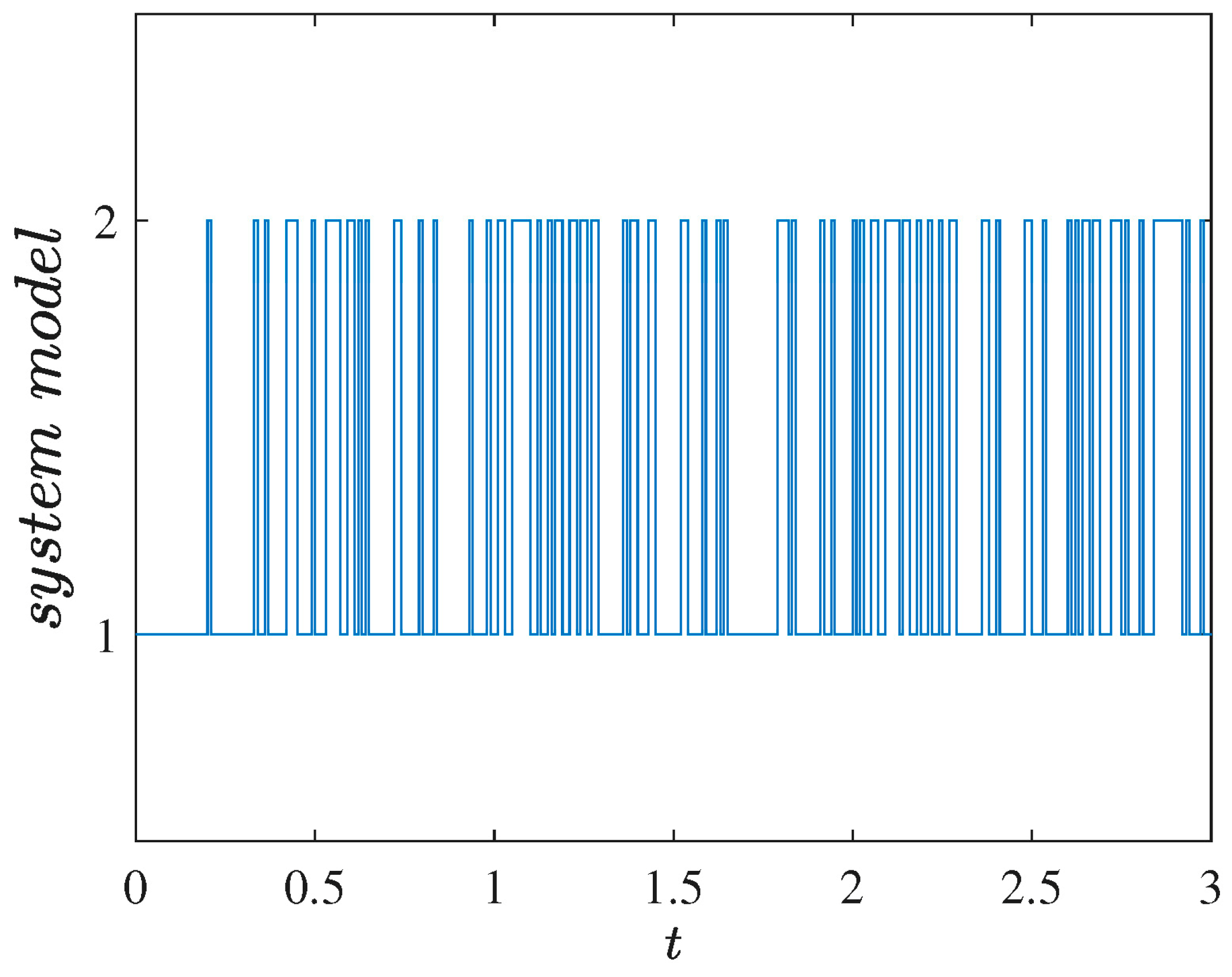
Example 1.

The node system of complex network is described by the chaotic system (47).

$$\{\begin{array}{l}{\dot{x}}_{i1}(t)=-x_{i1}(t)-x_{i2}(t)x_{i3}(t)+20x_{i3}(t)\\ {\dot{x}}_{i2}(t)=-x_{i2}(t)+x_{i1}(t)x_{i3}(t)\\ {\dot{x}}_{i3}(t)=5.45\left(x_{i1}(t)-x_{i3}(t)\right)\end{array}i=1,2,\dots ,N$$

(47)

This numerical simulation will compare the proposed optimal node selection strategy and event-triggered control strategy by numerical simulation of 20 nodes. In this simulation, the complex network, switching mode, and all parameters will remain consistent. The switching of two different modes in the complex network are shown in Figure 1, and the parameters of the network are also given in the following:

$$\begin{gathered} {\mathsf{\Gamma }}_1=[\begin{array}{ccc}0.5& 0& 0\\ 0& 0.5& 0\\ 0& 0& 0.5\end{array}],{\mathsf{\Gamma }}_2=\left[\begin{array}{ccc}0.8& 0& 0\\ 0& 0.8& 0\\ 0& 0& 0.8\end{array}\right],\mathsf{\Pi }=\left[\begin{array}{cc}-2& 2\\ 1& -1\end{array}\right], \\ \begin{array}{c}{\sigma }_i\left(t,e_i(t),1\right)=diag\left\{\frac{\sqrt{2}}{2}{e}_{i1}(t),\frac{\sqrt{2}}{2}{e}_{i2}(t),\frac{\sqrt{2}}{2}{e}_{i3}(t)\right\}\end{array} \\ \begin{array}{c}{\sigma }_i\left(t,e_i(t),2\right)=diag\left\{\sqrt{2}{e}_{i1}(t),\sqrt{2}{e}_{i2}(t),\sqrt{2}{e}_{i3}(t)\right\}\end{array}. \end{gathered}$$

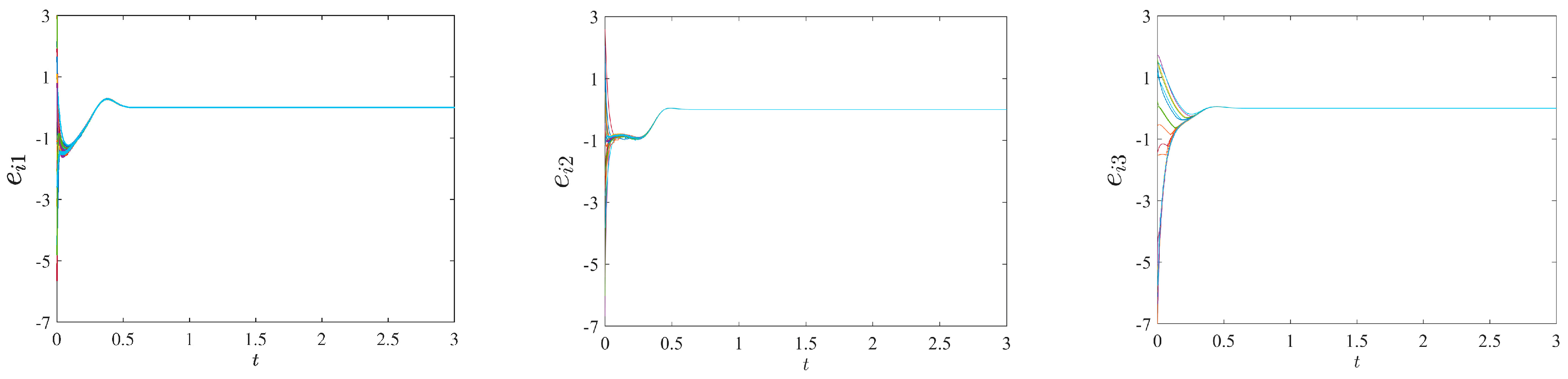
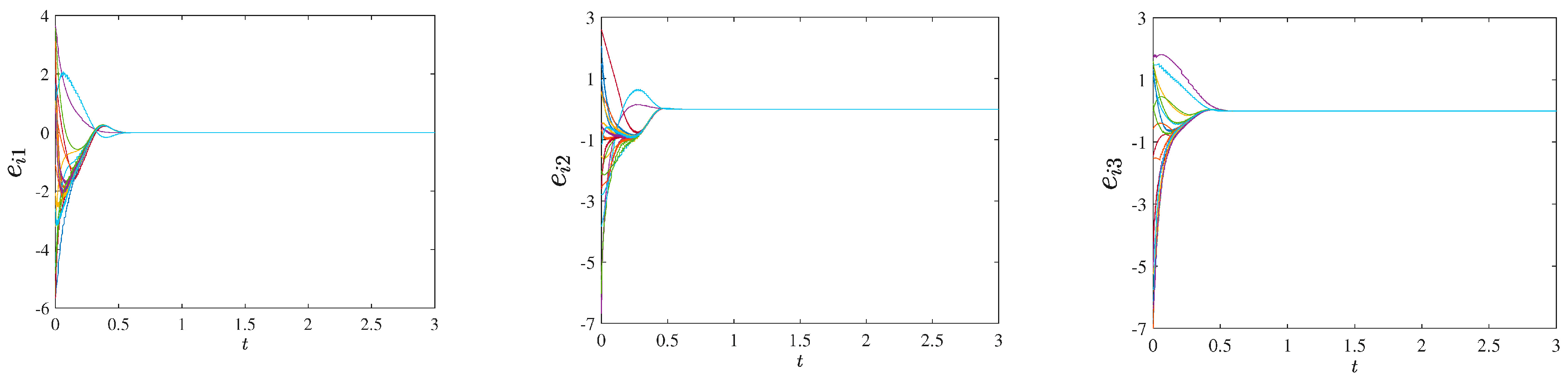
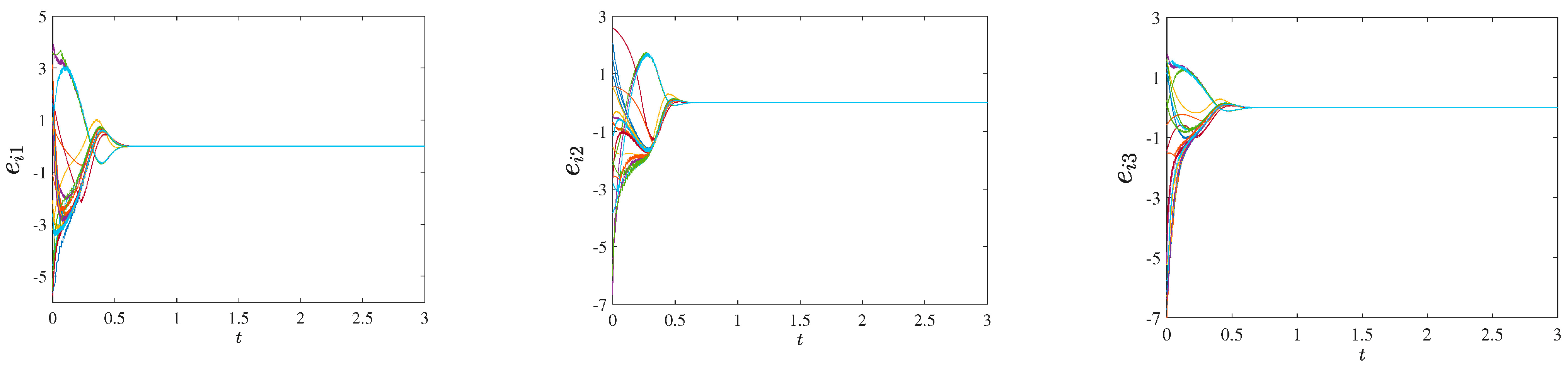
Example 2.

Finite-time synchronization of a multi-weighted Markovian switching complex network will be achieved by the optimal node selection strategy under different coupling strengths (c₁ = c₂ = 10, 1, 0.1, 0.001). The maximum average error node in each time interval (t_k−1, t_k] is selected as the control node. That is, only one node in the network is selected as the controlled node in this simulation, i.e., $u_i(t)=(u_1(t),\stackrel{20-1}{\overbrace{0,0,\dots ,0}})$, then the other control parameters in Theorem 1 are: η(1) = 90, η(2) = 100; φ(1) = 50, φ(2) = 45; β = 0.6; $\mathsf{\Xi }(1)=(90,\stackrel{20-1}{\overbrace{0,0,\dots ,0}})$, $\mathsf{\Xi }(2)=(100,\stackrel{20-1}{\overbrace{0,0,\dots ,0}})$; ρ(1) = 2, ρ(2) = 1.25. According to (13), we can get t^∗ ≤ 8.3147 by simple calculation.

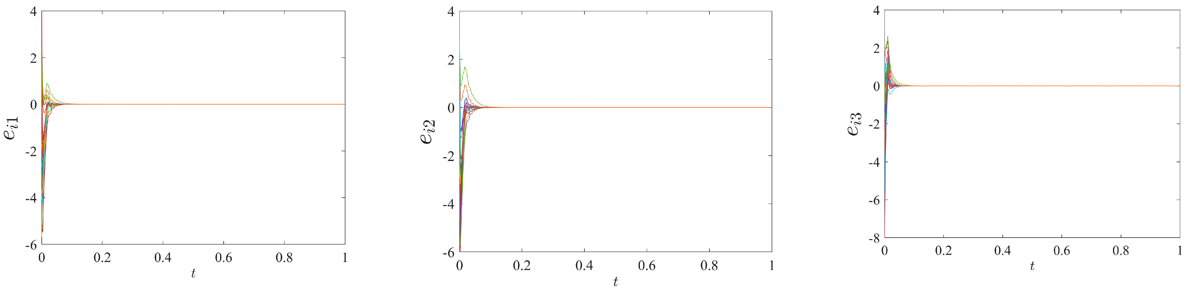
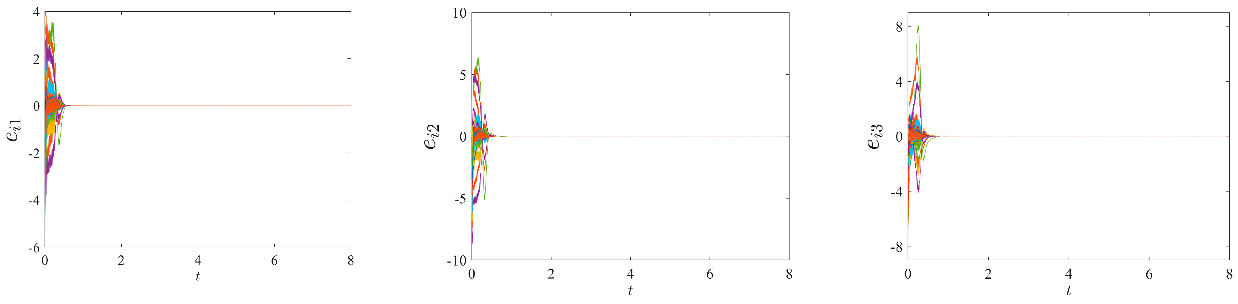
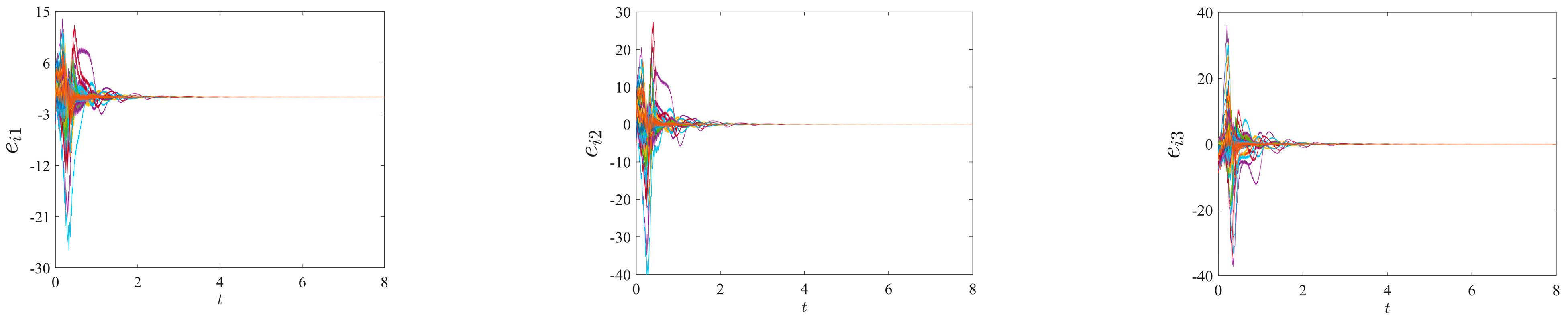
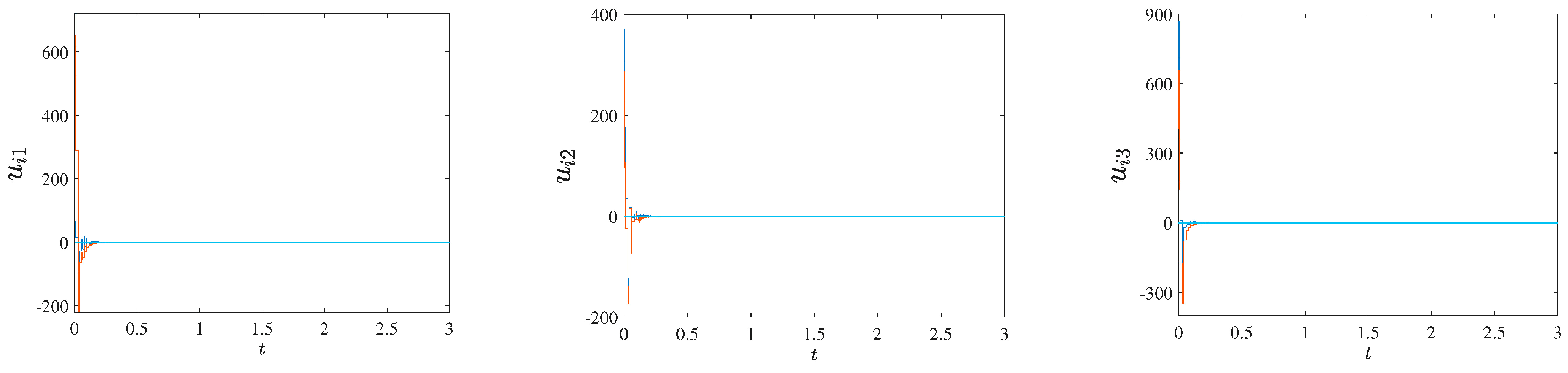
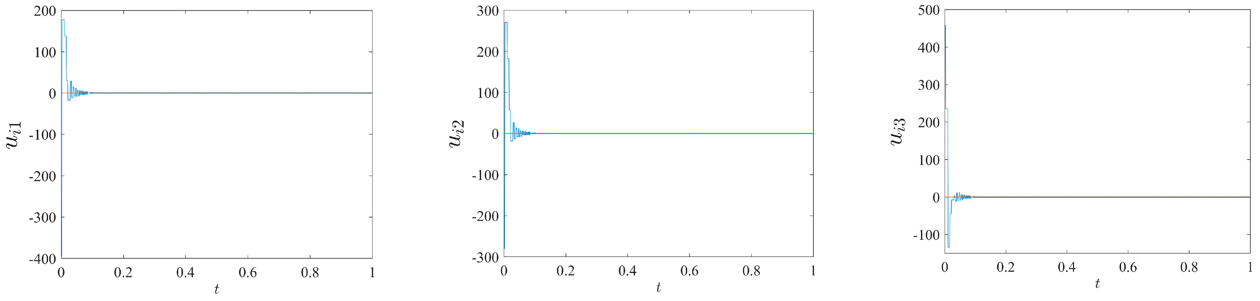
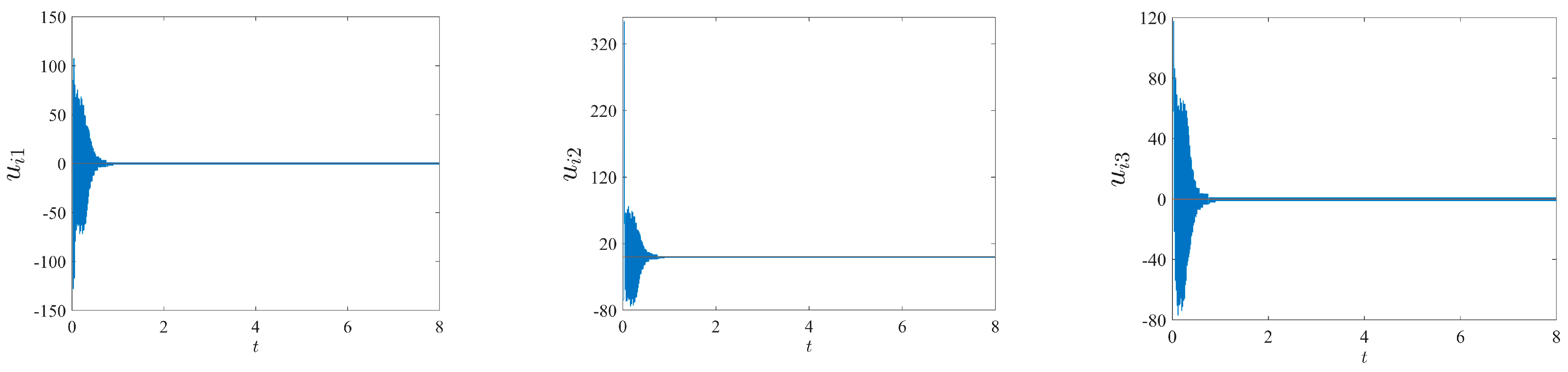
The evolution curves of the network synchronization error with time for different coupling strengths (c₁ = c₂ = 10, 1, 0.1, 0.001) are given in Figure 2, Figure 3, Figure 4 and Figure 5, respectively, from which it can be seen that the network synchronization error e_i(t) basically converges to 0 at t ≈ 0.6; Figure 6, Figure 7, Figure 8 and Figure 9 show the update process of the pinning controller with time for different coupling strengths (c₁ = c₂ = 10, 1, 0.1, 0.001), from which it can be seen that the designed controller u_i(t) are also gradually updated to zero at t ≈ 0.6. Then the synchronization of the multi-weight Markovian switching network can be achieved approximately at t ≈ 0.6. Therefore, under the optimal node selection strategy, when the coupling strength of the complex network changes, the synchronization time of the network does not change significantly.

In general, synchronization of complex networks can be achieved with very few of the control nodes when the coupling strength is large enough, or with a sufficient number of control nodes when the coupling strength is small. For the optimal node selection strategy proposed in this paper, not only the synchronization control of the complex network with Markovian switching is achieved with weak coupling strength (c₁ = c₂ = 0.001) and very few controlled nodes (1 controlled node), but also the synchronization efficiency of the network is improved, thus reducing the energy cost of the network.

Example 3.

In this simulation, finite-time synchronization of Markovian switching complex network will be achieved by the event-triggered control strategy under different coupling strengths (c₁ = c₂ = 10, 1, 0.4). According to the established event-triggered function to update the controller at all synchronization times, and the three nodes of the network are selected as controlled nodes, i.e., $u_i(t)=(\stackrel{3}{\overbrace{(u_1(t),u_2(t),u_3(t)}},\stackrel{20-3}{\overbrace{0,0,\dots ,0}})$. The parameter values in Theorem 2 are the same as those in Theorem 1. Especially, the control parameter ξ of the trigger function (31) is taken as ξ = 0.7; $\mathsf{\Xi }(1)=(\stackrel{3}{\overbrace{90,72,88}},\stackrel{20-3}{\overbrace{0,0,\dots ,0}})$, $\mathsf{\Xi }(2)=(\stackrel{3}{\overbrace{101,83,98}},\stackrel{20-3}{\overbrace{0,0,\dots ,0}})$. According to (34), we can get t^∗ ≤ 9.4628 by simple calculation.

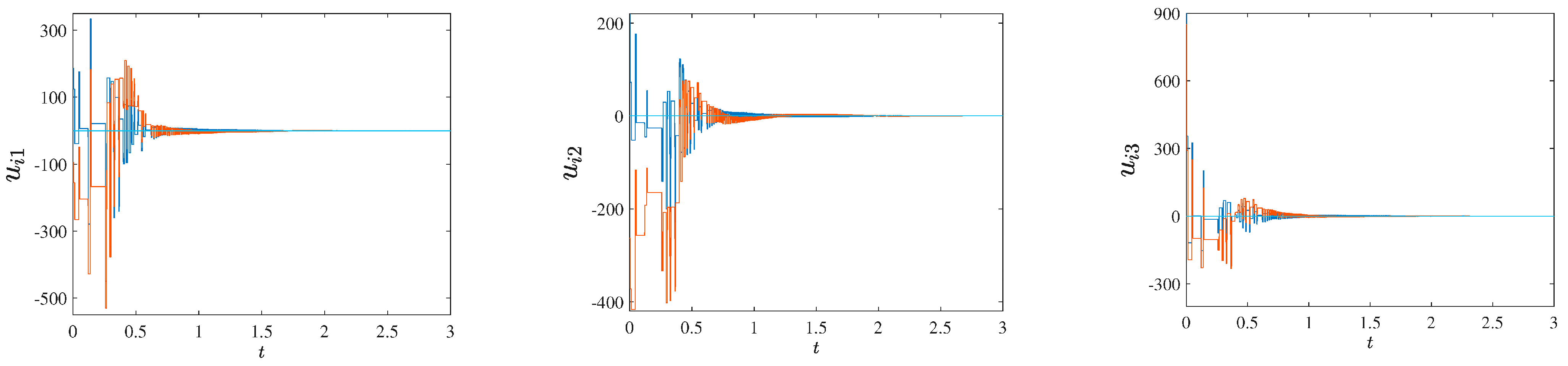
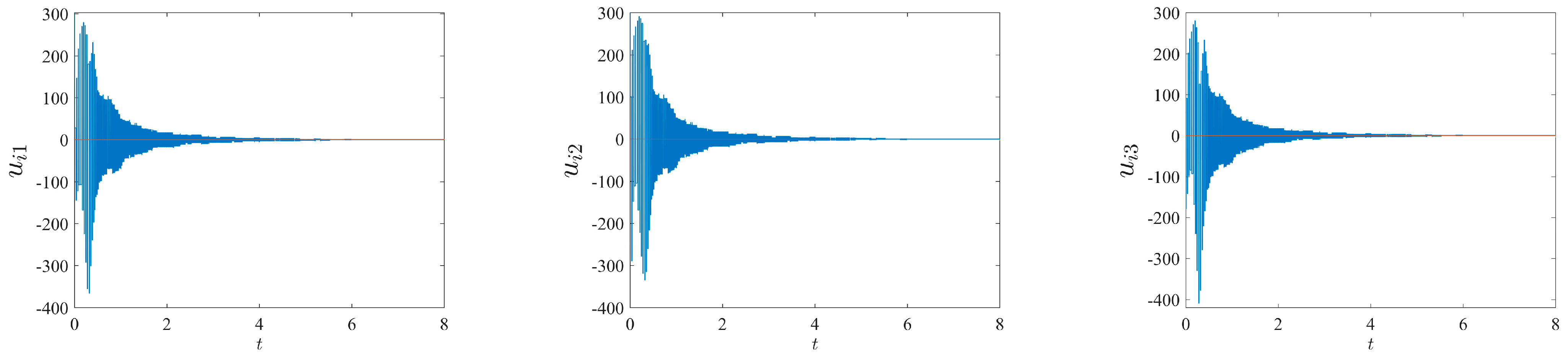
The evolution curves of the network synchronization error with time for different coupling strengths (c₁ = c₂ = 10, 0.1, 0.4) are given by Figure 10, Figure 11 and Figure 12 respectively; the update process of the event-triggered controller with time for different coupling strengths (c₁ = c₂ = 10, 0.1, 0.4) is given by Figure 13, Figure 14 and Figure 15, respectively. We can find that the synchronization error curves and the controller update curves of the system converge to zero at different network coupling strengths (c₁ = c₂ = 10, 1, 0.4) are different. Where synchronization of the Markovian switching network can be achieved at t ≈ 0.2 when the coupling strength c₁ = c₂ = 10, at t ≈ 1.2 when the coupling strength c₁ = c₂ = 1, at t ≈ 5 when the coupling strength c₁ = c₂ = 0.4. When the coupling strength of the network is very weak (less than 0.1 in Example 3), the Markovian complex network will no longer be synchronized under the event-triggered control strategy. Therefore, under the event-triggered control strategy, the synchronization time of the network gradually increases as the coupling strength of the network decreases.

The update process of the event-triggered controller is stepped, which is completely consistent with Remark 3. When the controller remains consistent, it means that the event trigger function condition is not satisfied, and the controller of the network remains unchanged at this time. When the controller appears to step up or down, it means that the set event trigger function is satisfied, and the controller of the network is updated at this time; thus, the theoretical analysis and the simulation results are also mutually verified.

Table 1. Comparison of the synchronization time of two control strategies in Example 1.

Control Strategy	Coupling Strength	Synchronization Time
Optimal node selection	(c1 = c2 = 10)	t ≈ 0.6
Event trigger control	(c1 = c2 = 10)	t ≈ 0.2
Optimal node selection	(c1 = c2 = 1)	t ≈ 0.6
Event trigger control	(c1 = c2 = 1)	t ≈ 1.2
Optimal node selection	(c1 = c2 = 0.1)	t ≈ 0.6
Event trigger control	(c1 = c2 = 0.1)	/
Event trigger control	(c1 = c2 = 0.4)	t ≈ 5
Optimal node selection	(c1 = c2 = 0.01)	t ≈ 0.6
Event trigger control	(c1 = c2 = 0.01)	/

shows the comparison of the synchronization time of the two control strategies in Example 1 (20-nodes network) with different coupling strengths.

The following conclusions can be obtained by analyzing the simulation results of Examples 2 and 3. When the network coupling is large enough (c₁ = c₂ = 10), the event-triggered control can achieve the synchronization of the network faster. When the coupling strength of the network gradually decreases (c₁ = c₂ = 1), the optimal node selection strategy can achieve the synchronization of the network faster. When the coupling strength of the network continues to decrease again (c₁ = c₂ = 0.1), the multi-weight Markovian switching complex network will no longer be able to achieve synchronization under the event-triggered control strategy. Moreover, the event-triggered control strategy controls three nodes of the network to achieve network synchronization, while the optimal node selection strategy only needs to control one node to achieve network synchronization, which can also reduce the control cost of the network. Therefore, when the actual system needs to achieve fast network synchronization with low control cost, the optimal node selection strategy can be used. When the actual system is not concerned with control cost but only needs to achieve faster network synchronization, the event-triggered control method can be used.

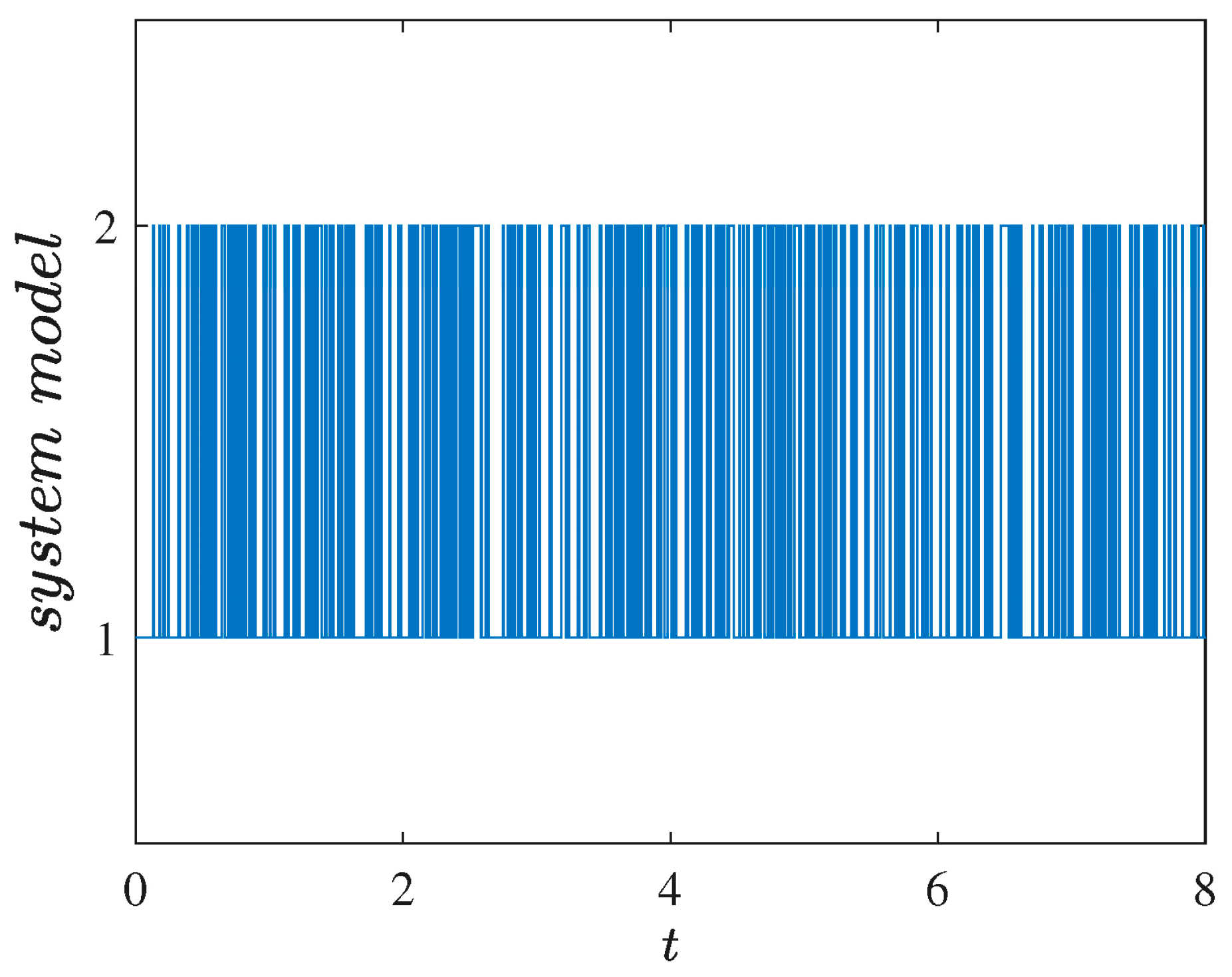
Example 4.

The node system of complex network is described by the Lorenz system (48).

$$\{\begin{array}{l}{\dot{x}}_{i1}(t)=10\left(x_{i2}(t)-x_{i1}(t)\right)\\ {\dot{x}}_{i2}(t)=28x_{i1}(t)-x_{i1}(t)x_{i3}(t)-x_{i2}(t)\\ {\dot{x}}_{i3}(t)=x_{i1}(t)x_{i2}(t)-\frac{8}{3}{x}_{i3}(t)\end{array}i=1,2,\dots ,N$$

(48)

In order to further illustrate the advantages of the optimal node selection strategy and the event-triggered control strategy, this section will adopt the 100-node Markovian switching complex network model for simulation. In this simulation, the complex network, switching mode and all parameters will remain consistent. The switching of two different modes in the complex network can be shown in Figure 16, and the parameters of the network are also given below.

$$\begin{gathered} {\mathsf{\Gamma }}_1=[\begin{array}{ccc}0.8& 0& 0\\ 0& 0.8& 0\\ 0& 0& 0.8\end{array}],{\mathsf{\Gamma }}_2=\left[\begin{array}{ccc}1& 0& 0\\ 0& 1& 0\\ 0& 0& 1\end{array}\right],\mathsf{\Pi }=\left[\begin{array}{cc}-2& 2\\ 1& -1\end{array}\right], \\ \begin{array}{c}{\sigma }_i\left(t,e_i(t),1\right)=diag\left\{\frac{\sqrt{2}}{2}{e}_{i1}(t),\frac{\sqrt{2}}{2}{e}_{i2}(t),\frac{\sqrt{2}}{2}{e}_{i3}(t)\right\}\end{array} \\ \begin{array}{c}{\sigma }_i\left(t,e_i(t),2\right)=diag\left\{\sqrt{2}{e}_{i1}(t),\sqrt{2}{e}_{i2}(t),\sqrt{2}{e}_{i3}(t)\right\}\end{array} \end{gathered}$$

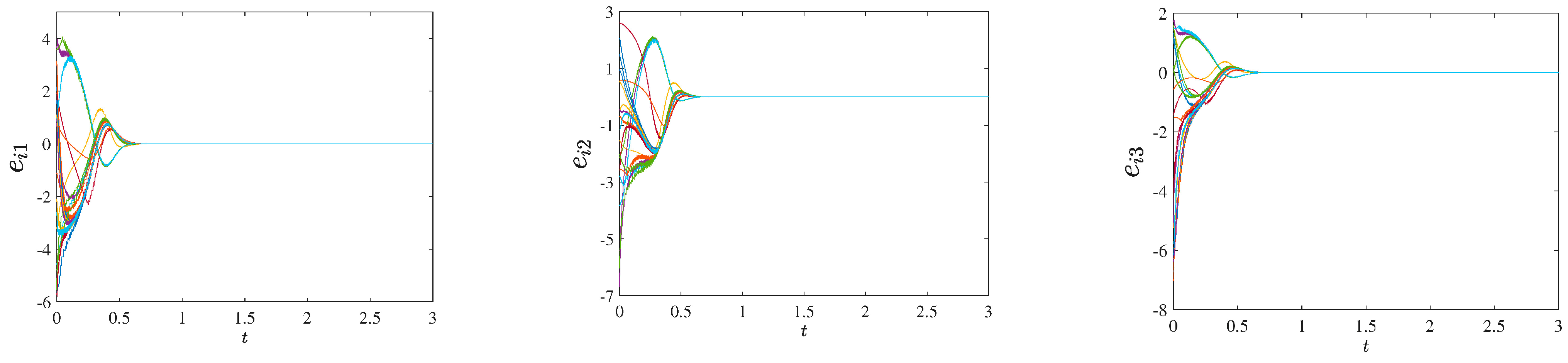
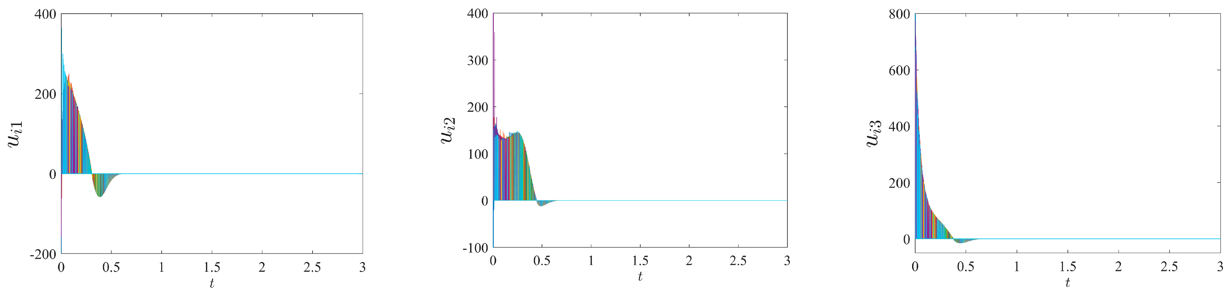
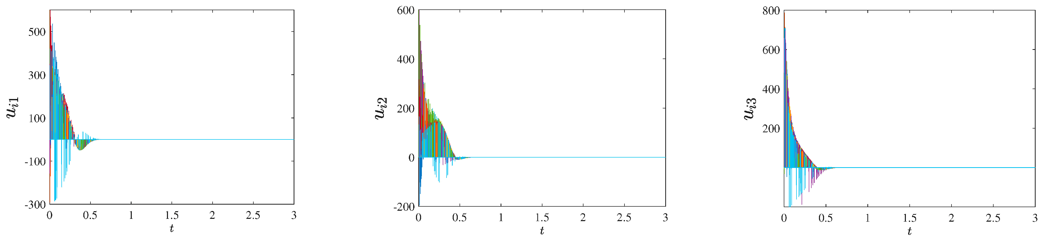
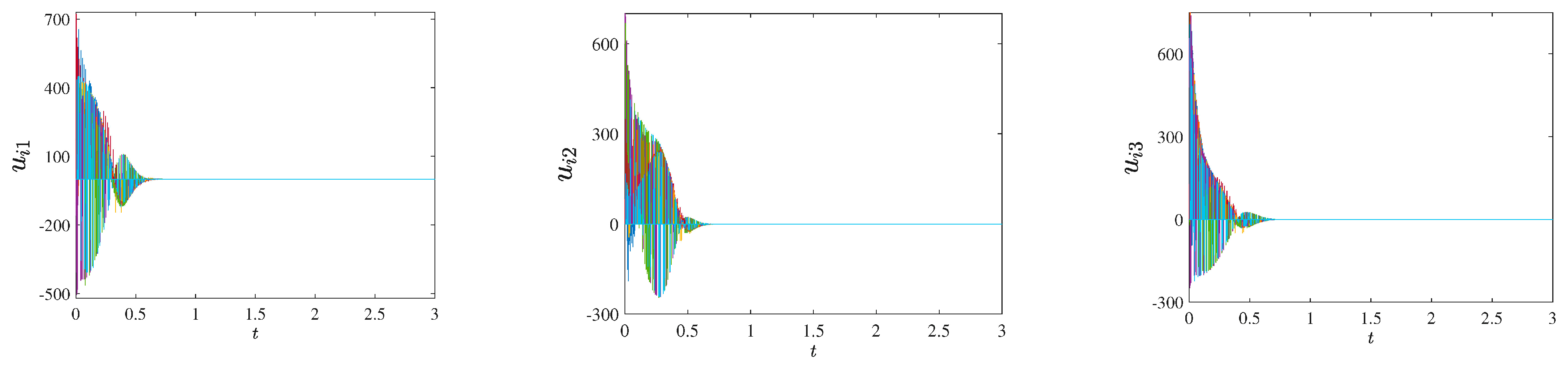
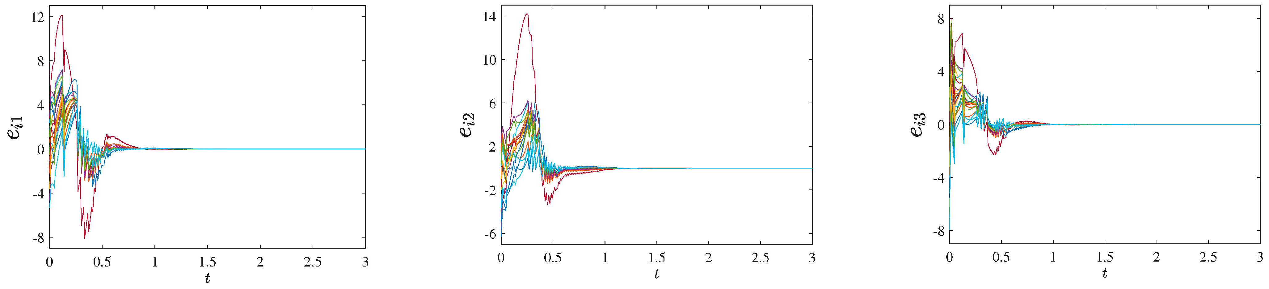
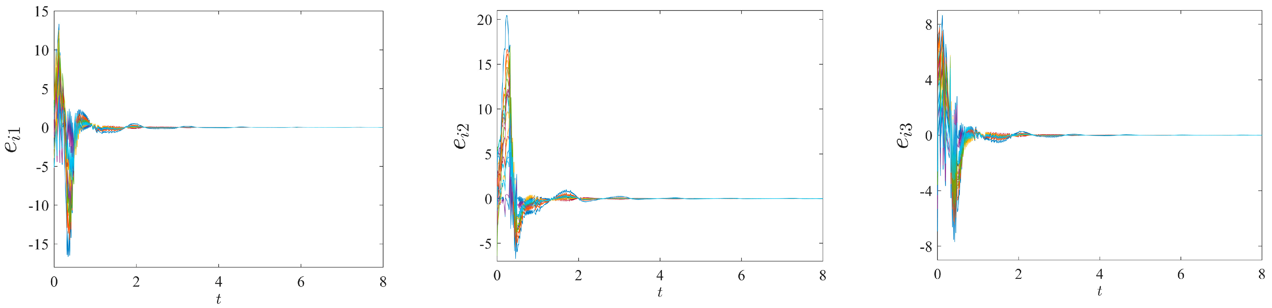
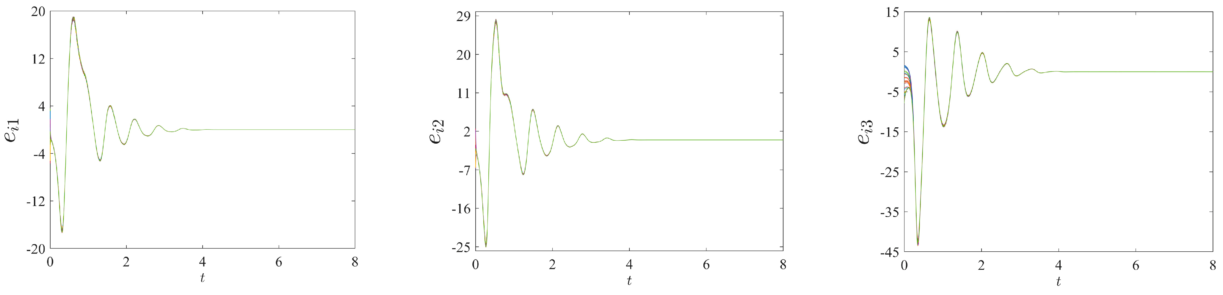
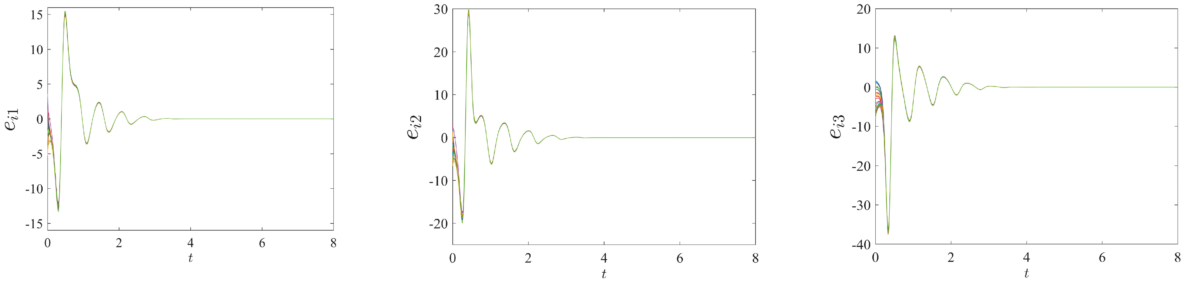
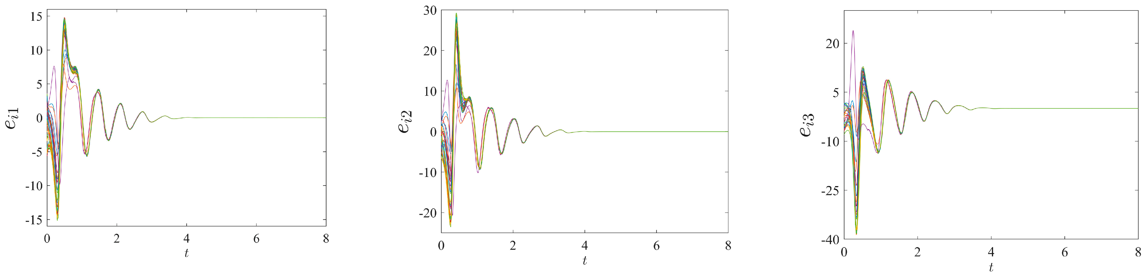
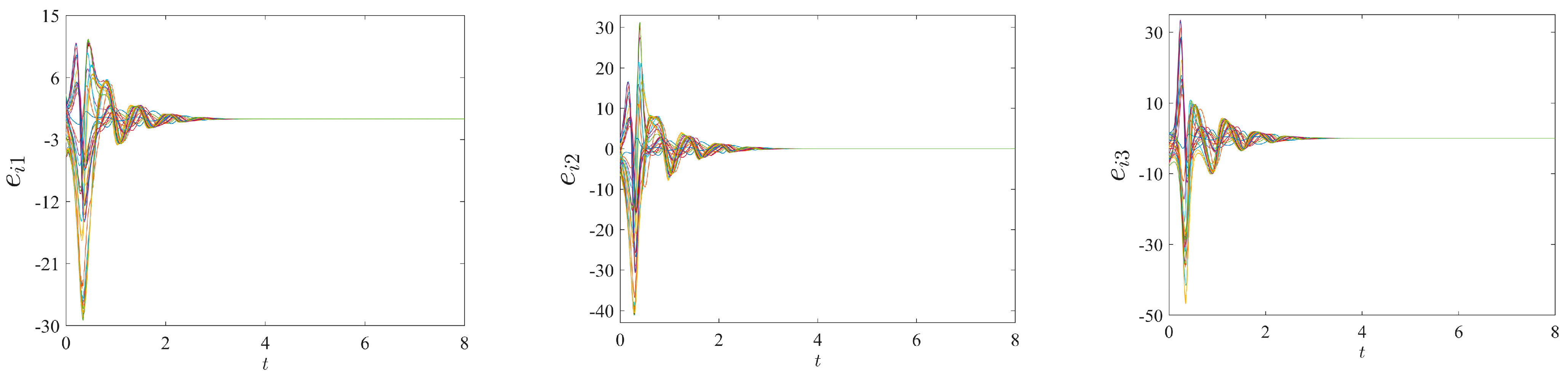
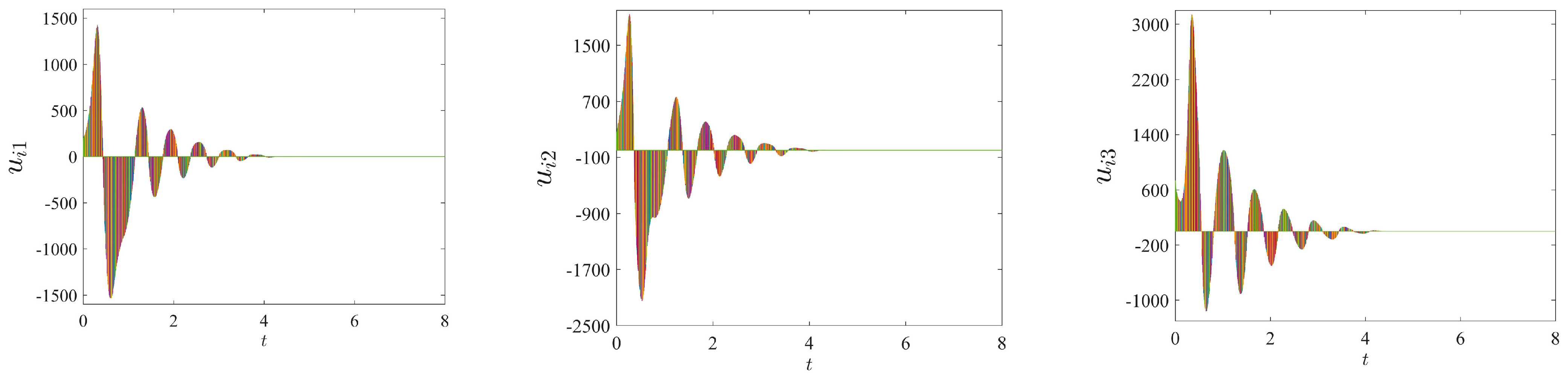
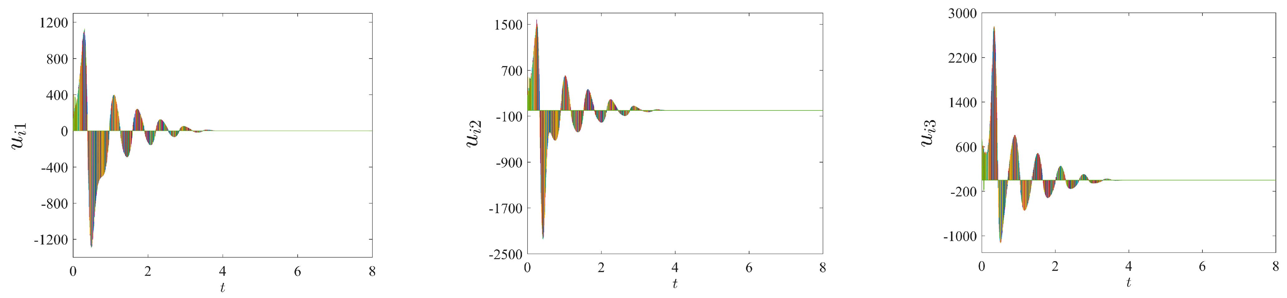
Example 5.

In this example, a multi-weight Markovian switching complex network model simulation with 100 nodes was performed using the optimal node selection strategy, and the coupling strengths of the networks were c₁ = c₂ = 10, c₁ = c₂ = 1, c₁ = c₂ = 0.1 and c₁ = c₂ = 0.001, respectively. The maximum average error node (only one node) in each time interval (t_k−1, t_k] is selected as the controlled node in this simulation, i.e., $\begin{array}{c}{u}_i(t)=(u_1(t),\stackrel{100-1}{\overbrace{0,0,\dots ,0}})\end{array}$, then the other control parameters in Theorem 1 are: η(1) = 90, η(2) = 100; φ(1) = 50, φ(2) = 45; β = 0.6; $\mathsf{\Xi }(1)=(90,\stackrel{100-1}{\overbrace{0,0,\dots ,0}})$, $\mathsf{\Xi }(2)=(100,\stackrel{100-1}{\overbrace{0,0,\dots ,0}})$; ρ(1) = 2, ρ(2) = 1.25. According to (13), we can get t^∗ ≤ 9.1316 by simple calculation.

Figure 17, Figure 18, Figure 19, Figure 20, Figure 21, Figure 22, Figure 23 and Figure 24 show the network synchronization error curves and the pinning controller evolution process under different coupling strengths (c₁ = c₂ = 10, 1, 0.1, 0.001), respectively, from which it can be seen that the multi-weight Markovian switching complex network basically converges to zero at t ≈ 4. This again verifies the conclusion obtained in Example 2. Based on the optimal node selection strategy, on the one hand, the network synchronization time does not change significantly with the change of the network coupling strength. On the other hand, synchronization can be achieved under weak coupling strength (c₁ = c₂ = 0.001) and very few controlled nodes (1 controlled node), which further reduces the network energy loss and control cost.

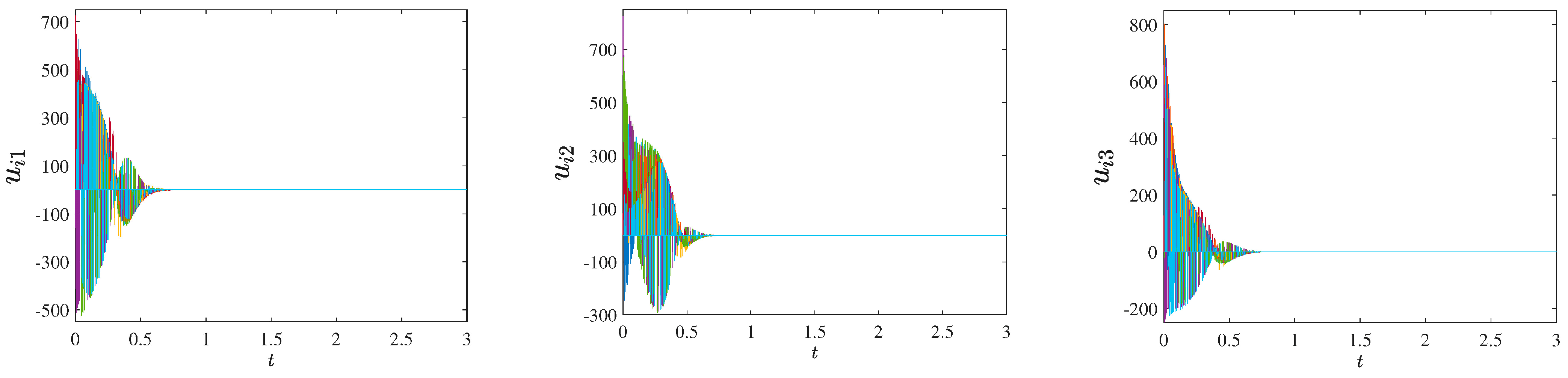
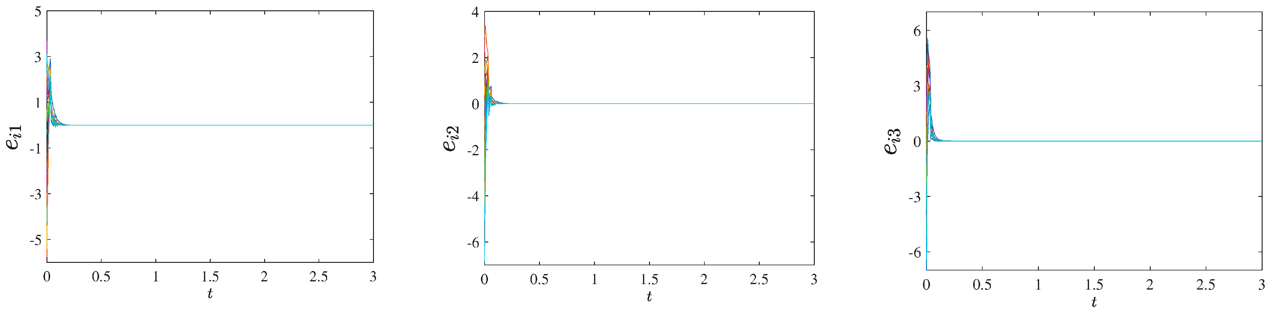
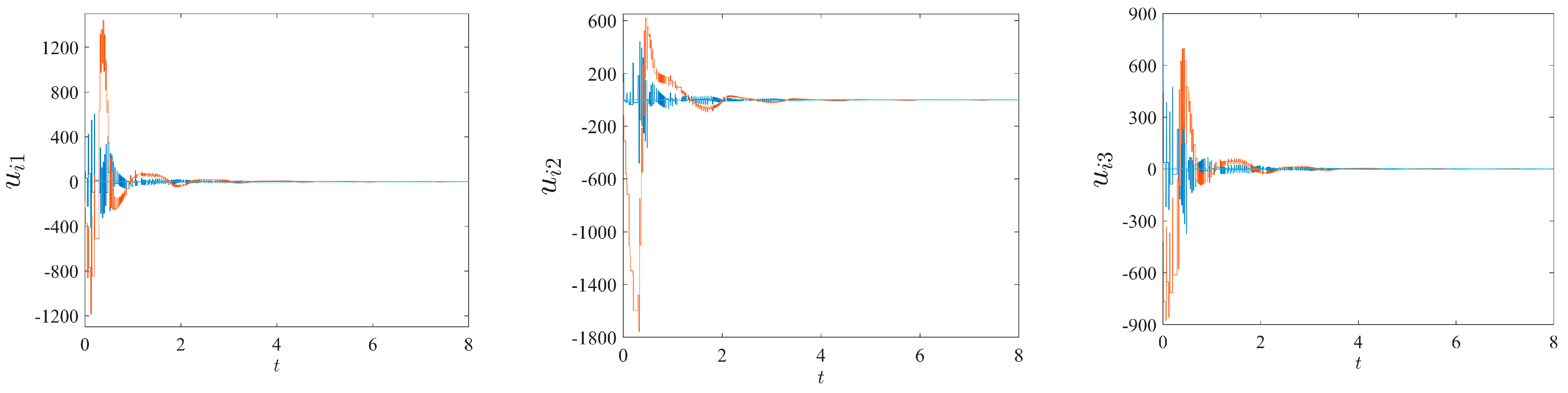
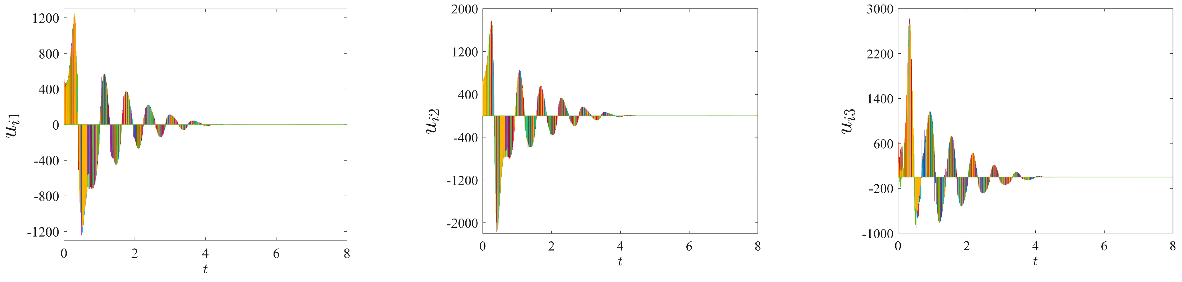
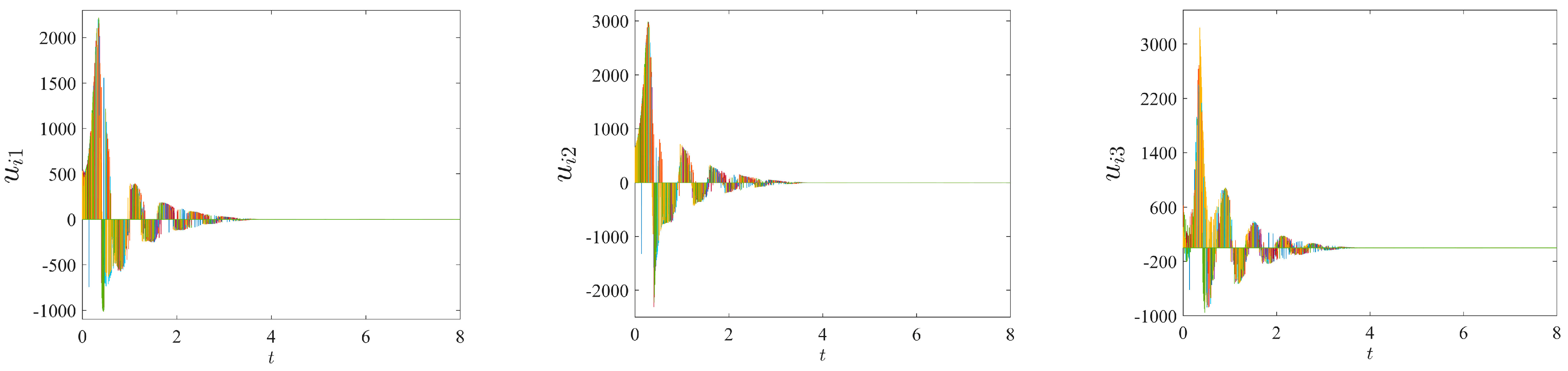
Example 6.

In this example, a multi-weight Markovian switching complex network model simulation with 100 nodes was performed using the event-triggered control strategy, and the coupling strengths of the networks were c₁ = c₂ = 10, c₁ = c₂ = 1, and c₁ = c₂ = 0.4, respectively. According to the established event-triggered function to update the controller at all synchronization times, and the three nodes of the network are selected as controlled nodes, i.e., $u_i(t)=(\stackrel{3}{\overbrace{u_1(t),u_2(t),u_3(t)}},\stackrel{100-3}{\overbrace{0,0,\dots ,0}})$. The control parameter ξ of the trigger function (31) is taken as ξ = 0.7; $\mathsf{\Xi }(1)=(\stackrel{3}{\overbrace{90,72,88}},\stackrel{100-3}{\overbrace{0,0,\dots ,0}})$, $\mathsf{\Xi }(2)=(\stackrel{3}{\overbrace{101,83,98}},\stackrel{100-3}{\overbrace{0,0,\dots ,0}})$. According to (34), we can get t^∗≤ 9.3369 by simple calculation.

The network synchronization error curves and the event-triggered controller update process for different coupling strengths c₁ = c₂ = 10, c₁ = c₂ = 1 and c₁ = c₂ = 0.4 are given by Figure 25, Figure 26, Figure 27, Figure 28, Figure 29 and Figure 30, respectively. Synchronization of the Markovian switching network can be achieved at t ≈ 0.1 when the coupling strength c₁ = c₂ = 10, at t ≈ 1.2 when the coupling strength c₁ = c₂ = 1, at t ≈ 5 when the coupling strength c₁ = c₂ = 0.4. When the coupling strength of the network is very weak (less than 0.1 in Example 6), the Markovian complex network will no longer be synchronized under the event-triggered control strategy. This again validates the conclusion obtained in Example 3. Based on the event-triggered control strategy, the synchronization time of the network gradually increases as the coupling strength of the network decreases, and the event-triggered controller is also step-varying.

Table 2. Comparison of the synchronization time of two control strategies in Example 4.

Control Strategy	Coupling Strength	Synchronization Time
Optimal node selection	(c1 = c2 = 10)	t ≈ 4
Event trigger control	(c1 = c2 = 10)	t ≈ 0.1
Optimal node selection	(c1 = c2 = 1)	t ≈ 4
Event trigger control	(c1 = c2 = 1)	t ≈ 1.2
Optimal node selection	(c1 = c2 = 0.1)	t ≈ 4
Event trigger control	(c1 = c2 = 0.1)	/
Event trigger control	(c1 = c2 = 0.4)	t ≈ 5
Optimal node selection	(c1 = c2 = 0.01)	t ≈ 4
Event trigger control	(c1 = c2 = 0.01)	/

shows the comparison of the synchronization time of the two control strategies in Example 4 (100-nodes network) with different coupling strengths.

The conclusions obtained in Example 1 can be verified again by analyzing the simulation results of Examples 2 and 3. When the coupling strength is large enough (c₁ = c₂ = 10, 1), the event-triggered control can achieve the synchronization faster. When the coupling strength gradually decreases (c₁ = c₂ = 0.1, 0.001), the Markovian complex network will no longer be able to achieve synchronization under the event-triggered control strategy, and the optimal node selection strategy can achieve the synchronization faster.

In addition to the above conclusions, by comparing Examples 1 and 4, it can be seen that as the number of network nodes continues to increase, the synchronization time of the network also increases under the optimal node selection strategy, and the time to achieve network synchronization under the proposed event-triggered control strategy will not change significantly as the number of network nodes increases.

6. Conclusions

This paper focuses on the analysis of low energy synchronization of Markovian switching complex networks through multiple perspectives. Analysis and discussion is based on the two control strategies of optimal node selection and event-triggered control.

(1)

Considering that the Markovian switching process will change the dynamic of the complex network, the optimal node selection strategy based on network node importance measurement is improved, and a controller with a simpler structure is designed, which can quickly achieve low energy synchronization of the complex network.

(2)

Considering the control cost problem caused by the large amount of information transfer between networks, a trigger function is designed that can eliminate invalid information intersection and transmission between networks based on the event-triggered control strategy, so as to achieve low energy synchronization of Markovian switching complex networks.

(3)

Based on the above two control strategies, important conclusions have been obtained through comparative simulation, which indicate that in order to optimally achieve synchronization control under low energy cost mechanism, a control strategy with faster synchronization speed and fewer control nodes is better.

I. Compared with event-triggered control strategy, the optimal node selection strategy can control less nodes (only one control node in Examples 2 and 5) to achieve network synchronization, which can further reduce the control cost of the network.

II. With the continuous increase of the network, the network synchronization time under the optimal node selection strategy has also increased. However, under the event-triggered control strategy, the time to achieve network synchronization will not change significantly with the growth of the network, but slightly more control nodes (three control nodes in Examples 5 and 6) are required compared to the optimal node selection strategy.

III. When the network coupling strength is large enough, the event-triggered control strategy can achieve synchronization faster. When the coupling strength of the network is very weak, the Markovian complex network can achieve synchronization faster under the optimal node selection strategy, and it will no longer be synchronized under the event-triggered control strategy.