Article

Optimization of the Flow of Parts in the Process of Brake Caliper Regeneration Using the System Dynamics Method

1
Department of Computer Science, Faculty of Mechanical Engineering and Aeronautics, Rzeszow University of Technology, Al. Powstańców Warszawy 8, 35-959 Rzeszów, Poland
2
Department of Production Computerisation and Robotisation, Faculty of Mechanical Engineering, Lublin University of Technology, Nadbystrzycka 36, 20-618 Lublin, Poland
3
Ph.D. School, Lublin University of Technology, Nadbystrzycka 38B, 20-618 Lublin, Poland
4
Department of Enterprise Organization, Faculty of Management, Lublin University of Technology, Nadbystrzycka 38, 20-618 Lublin, Poland
*
Author to whom correspondence should be addressed.
Processes 2024, 12(1), 16; https://doi.org/10.3390/pr12010016
Submission received: 22 November 2023 / Revised: 11 December 2023 / Accepted: 14 December 2023 / Published: 20 December 2023
(This article belongs to the Topic Modern Technologies and Manufacturing Systems, 2nd Volume)

Abstract

:
Remanufacturing processes are one of the key pillars of the so-called closed-cycle economy. Unfortunately, the design and organization of such processes pose a significant problem, due to, among other things, the high variability of the process as a consequence of both the degree of wear and tear and the quality of the remanufactured components. This article presents a method for optimizing the flow of the brake caliper remanufacturing process in the MTO (make-to-order) model. For the optimization process, the system dynamics (SD) method, which belongs to a group of simulation methods, was used. The developed model allows, in particular, the prediction of the number of components at the input to the regeneration process and the method of defining the size of the transport batch and evaluating its impact on the length of the production cycle of the batch of regenerated products. The issues of staffing management at individual positions and the organization of transport operations with variable production batch sizes were also discussed. The provided experiments have shown that reducing the size of the transport batch contributes to shortening the production order execution time, both with standard and increased staffing.

1. Introduction

As the world’s population grows, the demand for raw materials necessary for the production of various types of products increases [1,2]. However, this is becoming limited by the availability of natural resources, which poses a key challenge to paradigm shifts in the implementation of manufacturing processes [3,4]. Taking into account the finiteness of natural resources and the need to reduce the negative impact on the environment, the assumptions of a closed-loop economy, understood as a model of production and consumption, which is based on sharing, borrowing, reusing, repairing, renewing, and recycling existing materials and products for as long as possible, are becoming increasingly important [5,6].
A consequence of the growth of the closed-loop economy is the emergence and development of companies engaged in remanufacturing various types of products to enable their reuse [7,8]. Unfortunately, the organization of the flow in this type of processes is hampered, among other things, by the high variability of the process resulting, among other things, from the need to eliminate remanufactured elements at different stages of the process and the variability of the production batch size resulting from the reduction of elements subject to the remanufacturing process [9,10,11].
The classic model used in the remanufacturing of products is the make-to-stock (MTS) model, where the subject of planning is the number of products entering the process without regard to current customer needs [12]. Remanufactured products are directed to the finished goods warehouse, where they await customer orders [13]. Unfortunately, a consequence of this type of approach is the need to accumulate a large amount of inventory of remanufactured products, which entails storage costs, the need to freeze a large amount of financial resources and increases the risk of not being able to sell remanufactured products [14,15,16]. This is particularly important in the case of unique products, whose sales are characterized by low volumes [17,18].
In order to reduce the negative consequences of the implementation of the process in the MTS model, many companies are considering striving to change the model to the MTO model or the MTO–MTS hybrid model [19,20,21]. Unfortunately, the problem in this regard remains the correct planning of the number of products that should be introduced into the process so that, after taking into account the waste of defective products at subsequent stages, the number of products defined in the customer’s order is obtained at the end of the process [22,23]. The challenge of flow optimization also becomes the determination of the size of transport batches in such a way that the received order can be fulfilled on time [24,25,26].
In order to meet the above-mentioned requirements, this paper presents a method for optimizing the flow of the brake caliper body remanufacturing process in the MTO (make-to-order) model. A system dynamics (SD) simulation method was used for the optimization process.
The system dynamics (SD) method allows the analysis of systems composed of many components, linked by cause-and-effect relationships, often in the form of feedback loops, which makes it particularly useful in solving complex research questions [27]. The basis of the SD method is control theory [28] and systems thinking [29]. The SD method provides tools for numerical simulation and analysis of interactions between elements of the system under study. Extensive literature data indicate that the SD method is characterized by its versatile application, being useful in conducting the analysis of social, economic, and technical systems [30,31]. In the field of mechanical engineering, the SD method is now being introduced to carry out research in almost all stages of the product and technology life cycle [32,33,34,35,36,37,38].
Models of manufacturing systems made in the SD method are often realized at a high level of abstraction and need to be combined with other simulation methods. Studies that have attempted detailed simulation of manufacturing processes primarily introduce hybrid simulation—which combines the SD method with DES (discrete event simulation) or with ABMS (agent-based modelling and simulation) [39,40,41]. It has been shown that in numerical hybrid simulation, the SD method is primarily used to analyze supply chains, enterprises, and manufacturing systems at the strategic level. In contrast, detailed models of manufacturing systems are implemented using the DES or ABMS method.
The lack of detailed models of manufacturing systems developed by the SD method is mainly due to their considerable complexity [39,40,42,43]. Despite the finding of the initial trend of introducing the SD method mainly for the general analysis of manufacturing processes—without an accurate representation of the structure of the manufacturing process—the analysis of the literature data carried out indicates the possibility of using the SD method to accurately represent the elements of manufacturing systems. So far, using the SD method, among other things, models have been developed and numerical simulations have been carried out of: the performance of the machining process taking into account the change of basic cutting parameters (e.g., cutting speed, feed rate, and tool geometry) [44], the input hopper of a machine tool with a co-ordinated flow of material (FIFO—first in–first out), the readiness of the machine tool to process products [45], the implementation of the machining process on machine tools working in parallel and the combination of production flow and discretization of the flow of products [46,47]. The SD model’s representation of the operating parameters of the real production system has been shown to be highly consistent [44,48]. It was found that the results of SD simulation of a manufacturing system are more consistent with the behavior of the real system than in the case of DES simulation [48]. This provides an important rationale for extending the application of the SD method to the analysis of regeneration processes.

2. Materials and Methods

2.1. Problem Description

Due to the nature of remanufacturing processes, in the classic model, these processes are carried out in the MTS (make-to-stock) model, which, in practice, means the introduction into the process of a batch of used products determined on the basis of the production plan. The basis for the development of the production plan is the type and quantity of used components delivered to the production line by companies involved in the purchase of such components. In practice, this means that finished products (after remanufacturing) are collected at the output of the process, constituting a stock for later sale. Unfortunately, this type of approach (which is a classic push model) leads to the accumulation of a large amount of finished goods, which, consequently, results in high storage costs and a significant risk of not being able to sell the accumulated inventory.
Taking into account the above factors, companies are striving to change their production model towards the MTO model, which provides an opportunity to reduce the level of finished goods inventory, and, thus, the funds blocked in the remanufacturing process, as well as the storage costs and the risk of not being able to sell them. Unfortunately, the high variability of the process (including, among other things, the variable volume of waste of individual elements subject to the remanufacturing process, at different stages of the process) makes the planning process and organizing its flow become tasks that are difficult to implement in practice. The problem in this regard remains both the determination of the number of input elements to the process (because the number of products at the input will never be equal to the number of finished products), as well as the determination of the number and size of transport batches, which, due to the waste generated and the reduction of the size of the production batch, are dynamically changing.
In order to solve the problem thus defined, it was decided to use computer simulation methods. The subject motivating the research work undertaken was one of the international companies engaged in the remanufacturing of parts for cars and trucks. The enterprise carries out processes according to the MTS model, which results in the accumulation of a large volume of finished goods. In order to reduce warehousing costs, the enterprise is considering introducing production management in accordance with the MTO model, which involves changing the way production flow is managed. The peculiarities of the remanufacturing process cause difficulties in planning this process, and its correct organization requires answers to the following questions:
  • What should be the input number of items to the production system in order to fulfill a customer order without creating unnecessary inventory?
  • How to identify bottlenecks in the remanufacturing process and what actions should be taken to eliminate them (and, consequently, reduce the lead time of production orders)?
  • How to determine the size of the optimal transport batch in the case of decreasing number of items in the production batch?
In order to find answers to such defined questions (research problems), it was decided to carry out work involving modeling and simulation of the regeneration process using the system dynamics (SD) method. The process of regeneration of the brake caliper body was chosen as the object of research. The remanufacturing process of this key component of the brake caliper determines the possibility of fulfilling the customer’s order.

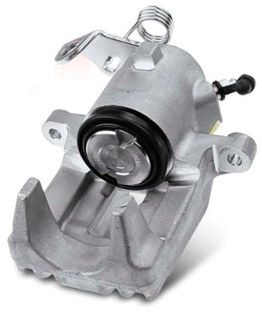
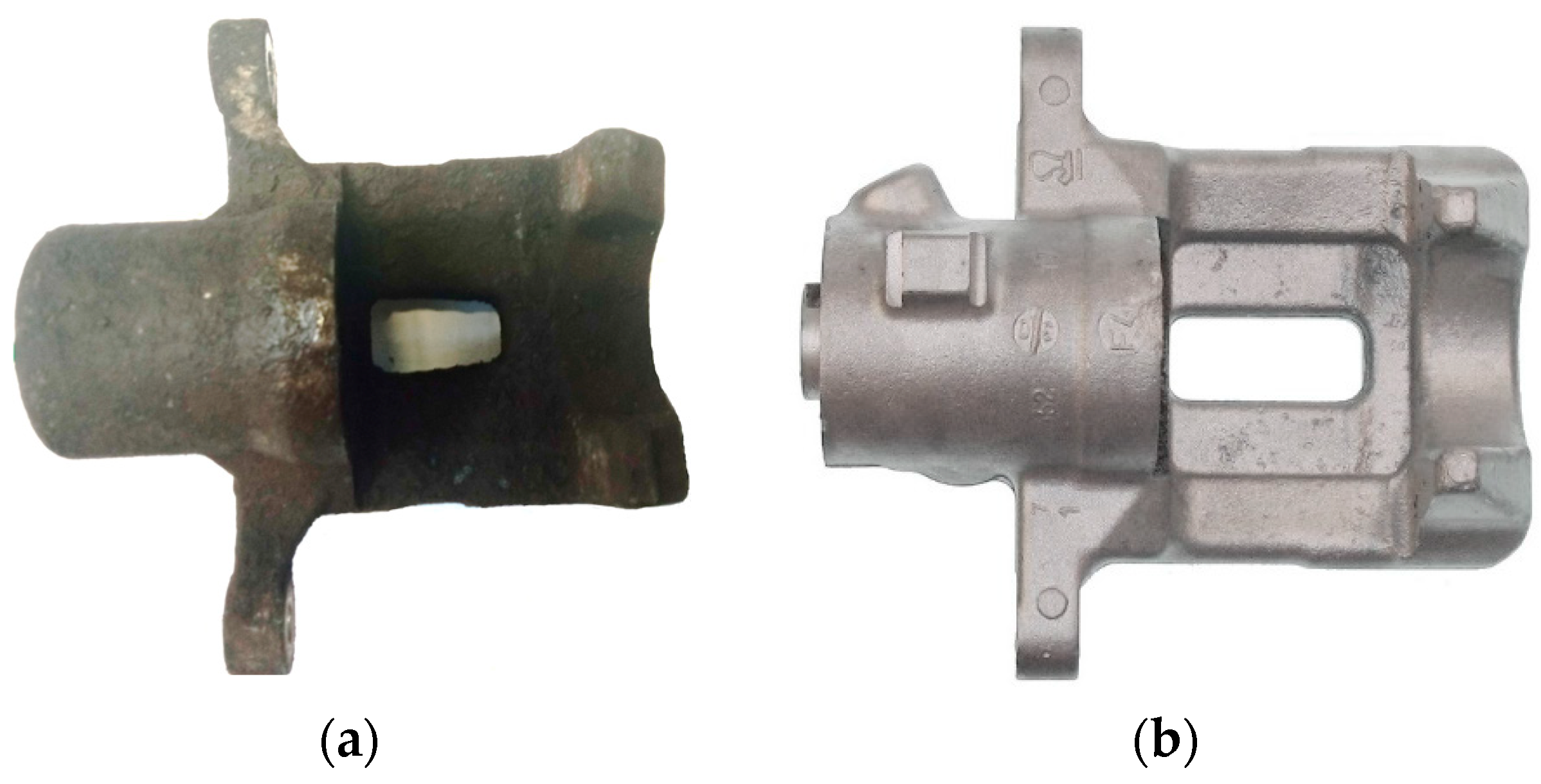
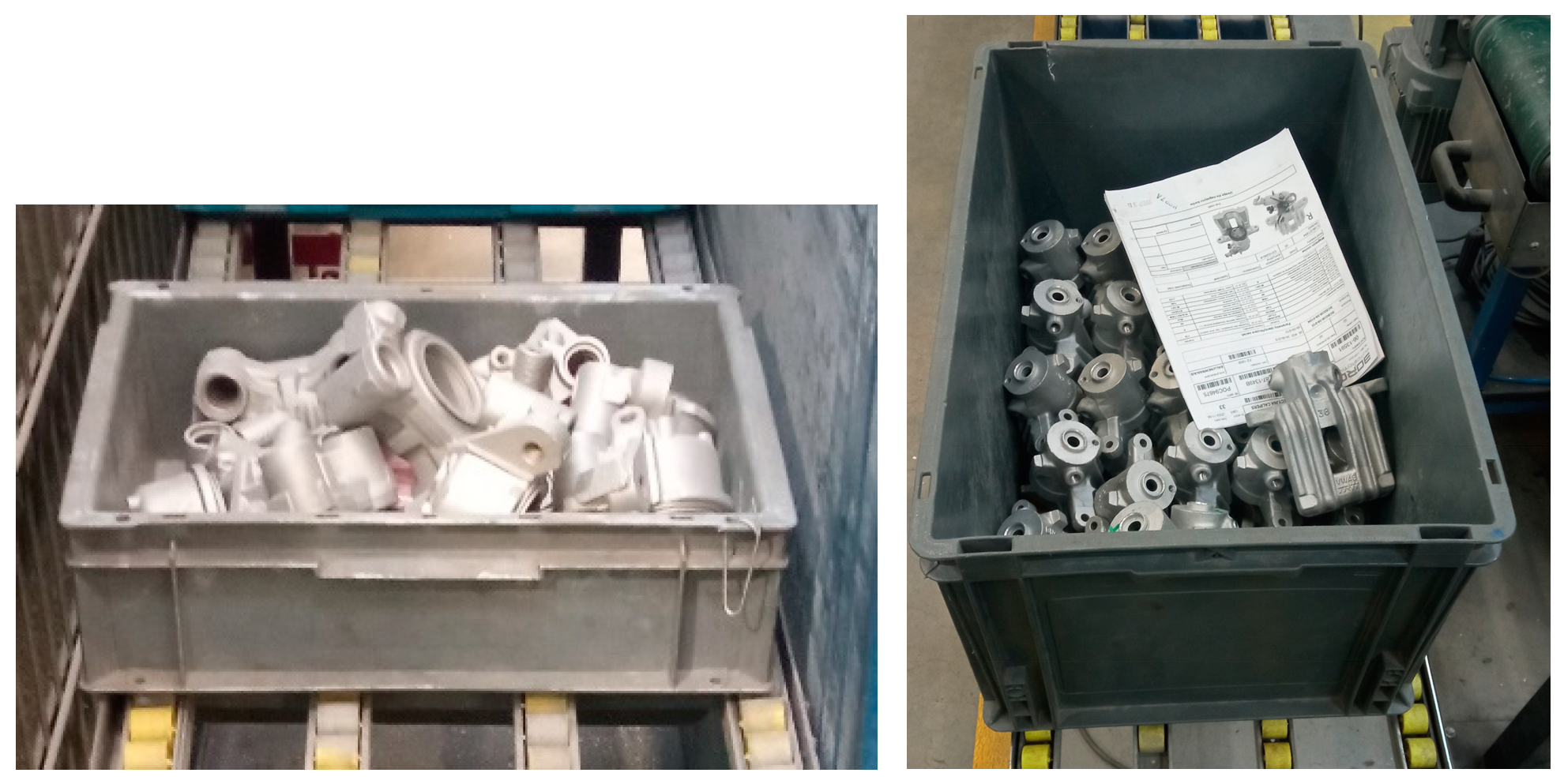
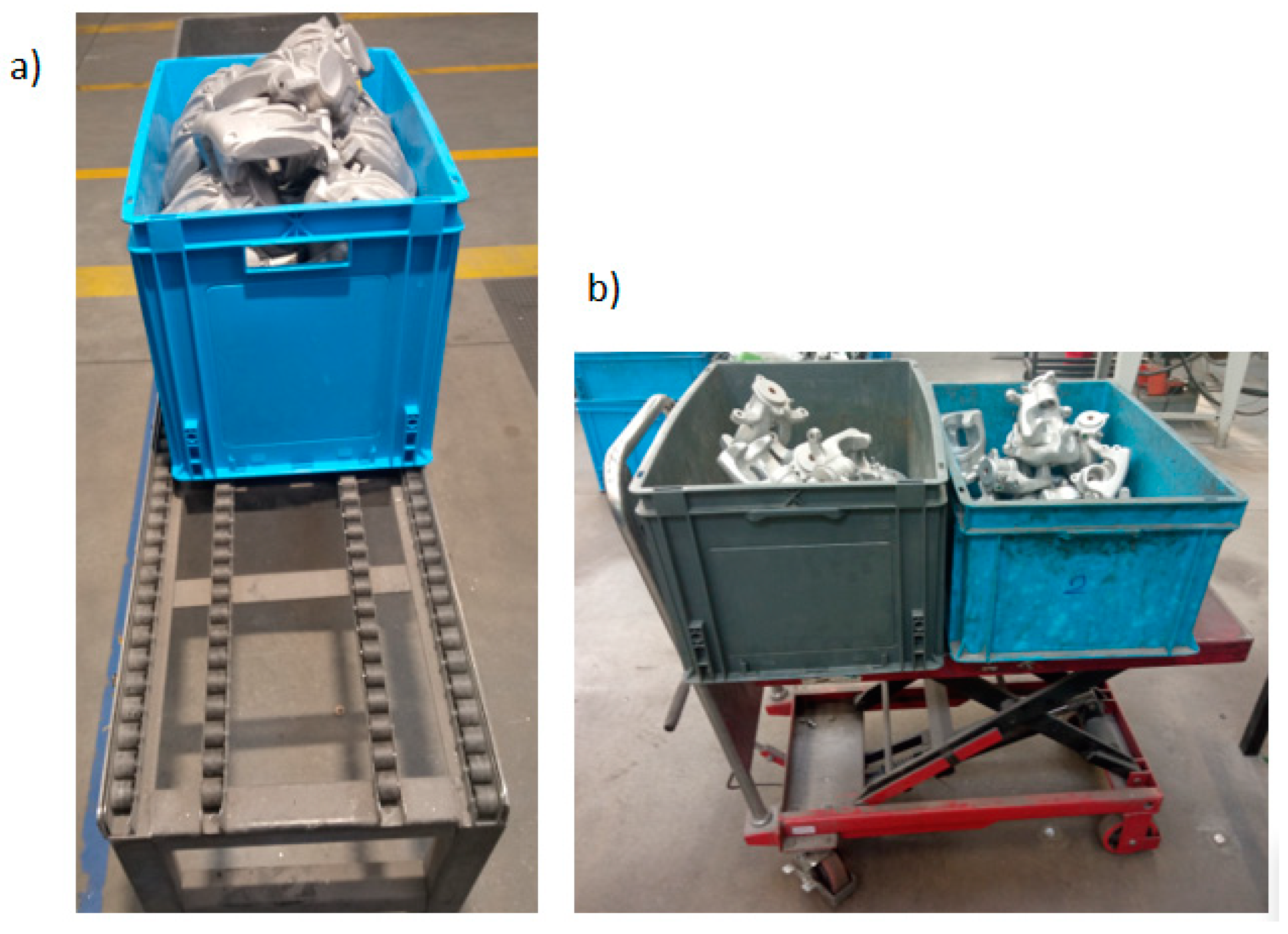
2.2. The Characteristics of the Brake Caliper Remanufacturing Process

The brake caliper (Figure 1) is a key component of the braking system in automotive vehicles that directly affects driving safety. The classic brake caliper consists of the following basic components:
-
Body;
-
Brake caliper piston;
-
Lever, bracket, and spring (in the case of handbrake);
-
Air vent.
Figure 1. Brake caliper.
Processes 12 00016 g001
The remanufacturing process aims to restore the product to its original state with possibly identical parameters as it had when it leaves the factory as a new product. This means that all components are individually checked at the entrance to the process and then subjected to a comprehensive remanufacturing. During remanufacturing, also new components are used that are impossible to restore to their original characteristics (e.g., bearings or rubber elements).
The correct performance of remanufacturing depends on proper planning of the process. The first task of the planning department is to determine the customer’s need for the product. Next, used brake calipers are sent to the disassembly station where the individual components of the product are separated. The components of the caliper are segregated accordingly and go to dedicated remanufacturing lines. One of the components of the caliper is its body, the regeneration process of which is the focus of this work (Figure 2).
The general scheme of the process of regeneration of brake caliper bodies is shown in Figure 3. The whole process begins with the disassembly of the brake caliper (P1).
The disassembly process is followed by body washing (P2). Contaminants in the form of dust, grease, corrosion, and other impurities that have formed during the operation are removed.
The next step is sorting and verification (P3). This is the point at which the bodies are thoroughly inspected for quality. The condition of critical components is verified and the brake caliper body is also checked for excessive corrosion. In case of a negative assessment of the quality of the body, it is scrapped.
After passing the sorting, the regeneration of surfaces responsible for the proper adhesion of brake pads (P4) is carried out. During the operation of the calipers, these surfaces are worn unevenly, which results in a deterioration of braking efficiency. The regeneration operation is carried out with customized machine tools (saws).
After transferring the body to the next workstation, the regeneration of threaded holes (P5) occurs. Successful regeneration ensures that there will be no leaks or problems with the installation of the brake caliper in the car. Nevertheless, it sometimes appears that repair is not possible. The bodies are then transferred to CNC milling machines or scrapped.
A series of machining operations (P6) are carried out on CNC milling machines. Threaded holes are repaired here by inserting repair bushings. Hydraulic system connections, air vent, piston adjustment mechanism, and lever shaft holes are regenerated.
These processes are followed by a comprehensive quality control (P7). It is aimed at detecting any defects that arise during remanufacturing.
The next step is to improve the visual characteristics of the body (P8). For this purpose, a special putty is used. After it is applied to the areas of corrosion defects and its hardening, it is carefully grinded and painted.
Puttying is the last dirty process, followed by body washing (P9). Clean details begin the preassembly stage, part of which is the insertion of sleeves (P10). Next comes the completion of the necessary components of the caliper, i.e., bolts, gaskets, pistons, etc. (P11).
When all components are prepared, they go to the assembly where they are carefully assembled giving the final complete brake caliper (P12).
The final stage is verification of the caliper at the final test. Here the integrity of the system is checked, as well as the visual quality of the body and the compatibility of the installed components (P13). After a positive final test, the remanufactured calipers go to the warehouse from where they are then distributed to customers.
Correct regeneration of the caliper is not always possible. Some of the items are excessively worn—they have defects, which, when identified, lead to production waste. According to the company, waste is identified in the following processes: sorting, sawing, and quality control. Regenerated calipers are not always subjected to all technological operations (omission of selected operations is possible in the case of good quality of individual features of the product, eliminating the need for regeneration)
Figure 4 shows the average waste values of defective parts, the quality of which prevents their regeneration. As can be seen from this diagram, after the sorting operation, an average of 15% of the clamps is production waste, 17% is sent to the next operation—cutting, the remaining 68% does not require surface recovery and is sent to the threading operation (P5). After surface regeneration (P4—saw), 98% of the parts go to the next operation—threading (P5), and 2% are identified as production waste. After threading, 85% of the calipers are moved to the CNC operation, and 15% are sent directly to quality control. After CNC processing, about 2% are production waste. In the quality control operation, an average of 69% of the clamps are sent for cleaning, 30% are sent for putty application, and 1% are identified as scrap. Production waste is also identified by the leak test performed after the final process step (clamp assembly and test). They amount to about 1% of the parts tested.
An important factor affecting the efficiency of the flow of products during the remanufacturing process is the interoperational transport processes. In the analyzed process, items are transported in transport boxes (Figure 5), the size of which is adjusted to the number of pieces in the transport batch.
The transport of bodies between the various stages of the regeneration process is carried out using two transport devices, i.e., a roller conveyor (Figure 6a) and a scissor transport truck (Figure 6b). The roller conveyor system allows transport in a way that is more ergonomic for the operator and more efficient in terms of transport time. Scissor transport carts, on the other hand, allow the load to be raised and lowered to different heights. Thanks to this flexibility, these devices are ideal for areas where manipulation and transport flexibility are needed.
The diverse construction of the stations where various regeneration operations are carried out imposes the necessity of adapting the means of transport to the specifics of the area, which makes both roller conveyors and scissor transport trucks applicable to different stages of the brake caliper remanufacturing process.

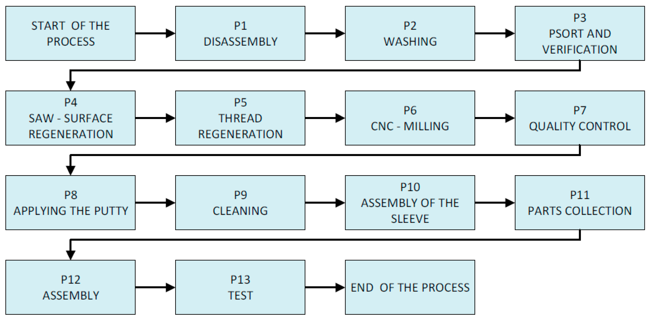
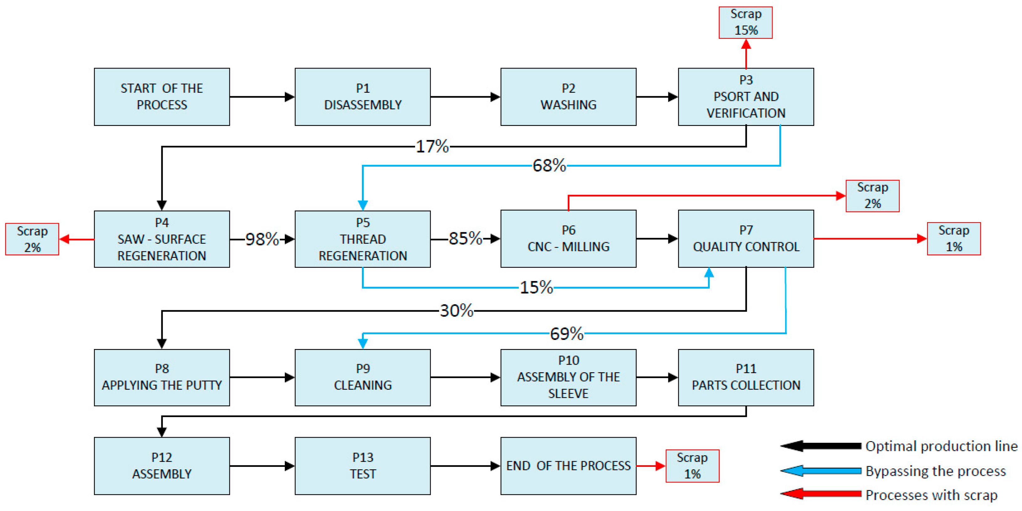
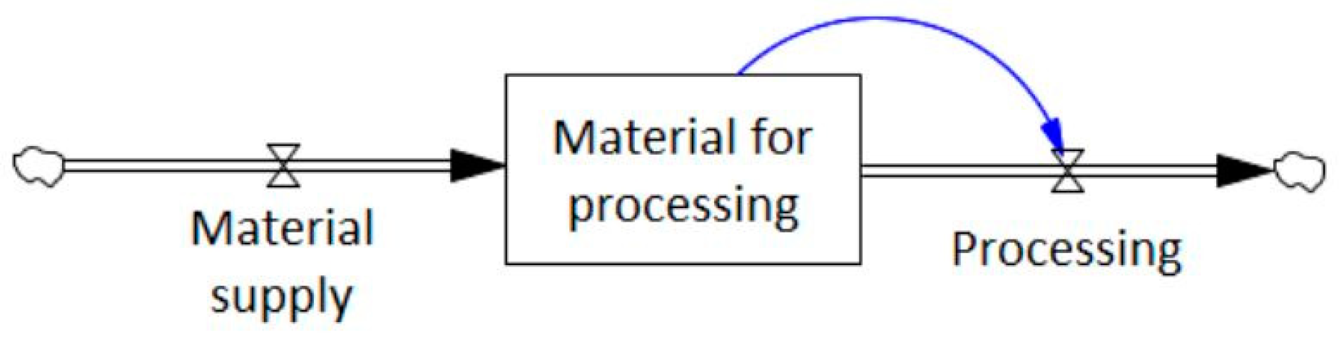
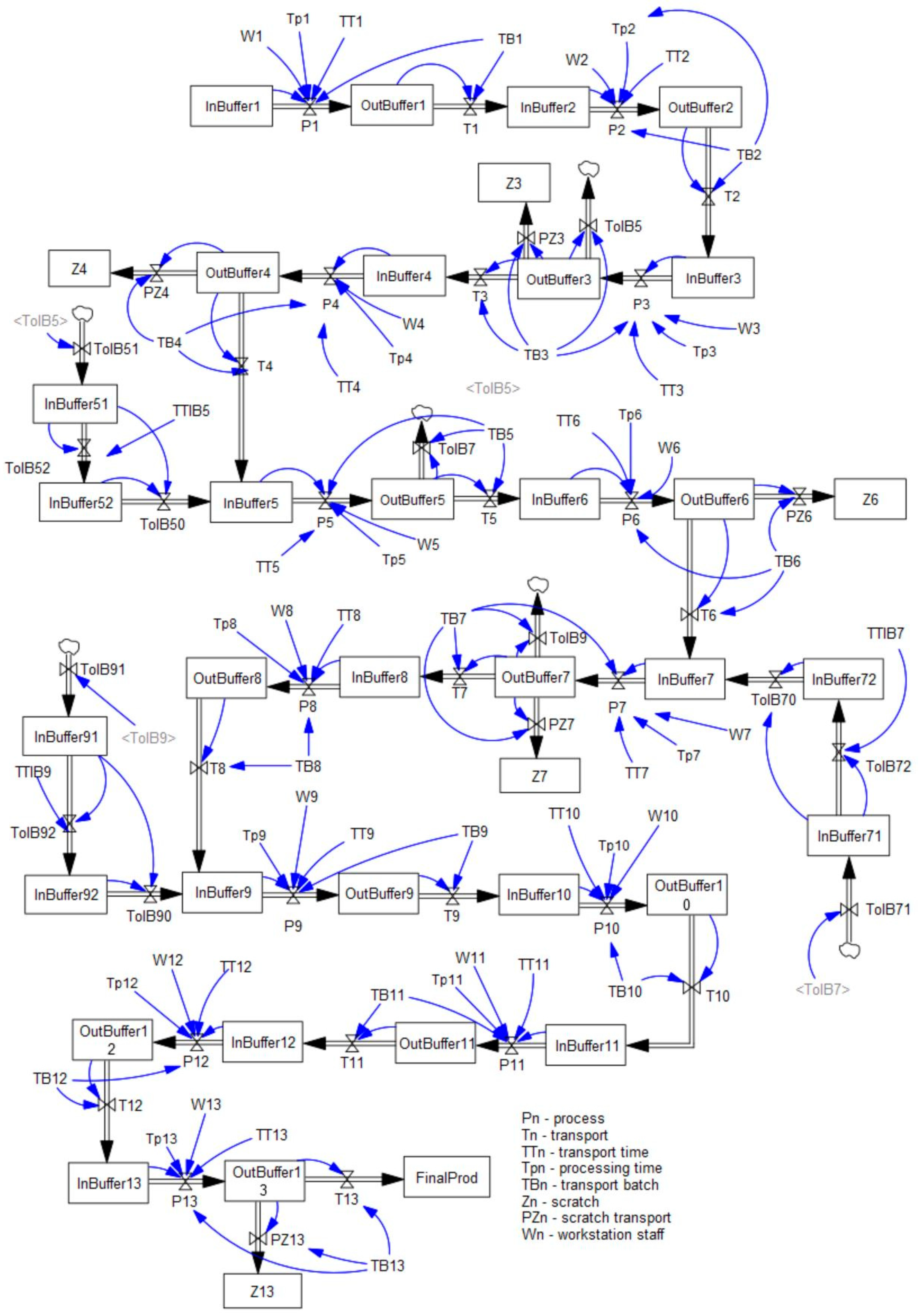
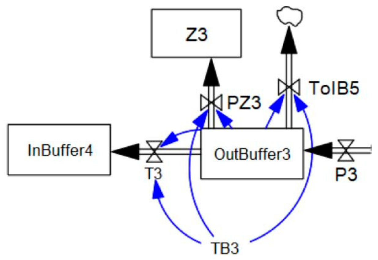
3. Modeling the Brake Caliper Body Remanufacturing Line with the Use of the System Dynamics Method

The system models created by the SD method include two basic categories of elements: stocks and flows, and the cause-and-effect relationships linking these elements. A stock represents the instantaneous value of an element in the modeled system, while a flow defines the rate of change of a stock. A schematic of a manufacturing workstation structure typically includes a stock Material for processing with two flows: Material supply and Processing (Figure 7). The stock is the same as any storage (inventory) of processed products. The flows represent material transfer and processing operations, respectively, increasing or decreasing the value of the stock. The dependency curve linking the stock Material for processing and the flow Processing indicates the relationship of these elements—processing occurs when materials are available.
The basis for developing a model of the brake caliper body remanufacturing process in the convention of system dynamics was a schematic of the brake caliper remanufacturing process, data on the average volume of waste at each stage of the process (Figure 4), the table of process operation times (Table 1), the table of transport operation times (Table 2) and a description of the production flow presented in Section 2.2.
Measurement of unit time and transport operation time was performed using the chronometric method and included the following steps:
  • Process observation: defining the areas and key elements for which measurements should be made;
  • Measuring the time: time measurement was conducted using a stopwatch. Measurements began with the start of a specific operation and ended with the completion of the same operation;
  • Uncertainty analysis: due to the unique form of the regeneration process, the operation times may have some uncertainty and measurement imprecision. Differences in operating conditions, job specifics, or technologies used can affect the duration of individual operations;
  • Measurement repeatability: in order to obtain more reliable results, the postmeasurement time of regeneration operation was recorded repeatedly. Multiple measurements allow estimation of the time range and help identify possible deviations.
Due to the measured times of technological and transportation operations, in many cases less than a minute in the model, 1 s was adopted as the basic unit of time. The results of the simulation experiment were recorded at each time step, i.e., every second. The simulation time of the brake caliper remanufacturing process depended mainly on the throughput of the production stations and the size of the production and transportation batch, and ranged from 24,000 to 69,000 s. Due to the abrupt changes in the values of the flow streams (e.g., the start of the transport operation after the required amount of material has been collected), the Euler integration technique was adopted during the simulation.
The model of the brake caliper body remanufacturing process was developed in Vensim Professional 7.2 software (Figure 8).
Each process operation has been connected to two storage bins, from which it takes and to which it transfers the processed clamp body. For example, operation P1 (disassembly) is connected to the InBuffer1 and OutBuffer1 storage bins. The item is transferred from the OutBuffer of the preceding operation to the InBuffer of the following operation in the transport process (T1, …, T13). If, according to the description of the production flow of a technological operation, nonconforming products are produced, then a flow of products is realized from the output storage bin of this operation to the waste storage location (Z3, Z4, Z6, Z7, and Z13). Such a flow reduces the number of products transferred to the next operation. In addition, some products can skip selected technological operations (processing is not necessary). This can be seen in the example of operation P5—THREAD REGENERATION, after which part of the body goes to P7—QUALITY CONTROL bypassing P6—CNC MILLING (which corresponds to the specifics of the process shown in Figure 4). The movement of products from the process P5 to P7 is represented by the flow ToIB7, which causes a decrease in the flow T5, and an increase in the state of the InBuffer7.

4. Simulation of the Flow of Parts in the Process of Regeneration of Brake Caliper Bodies

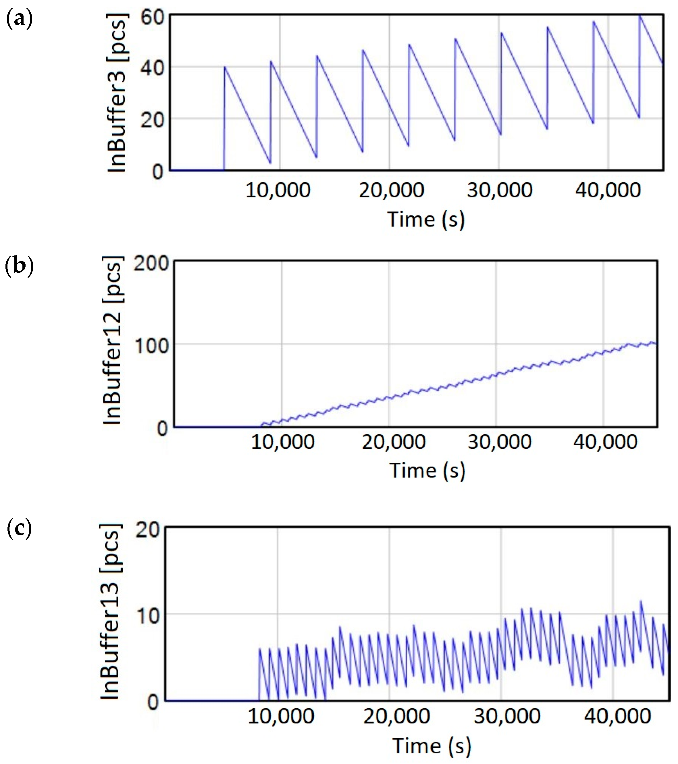
4.1. Determination of the Number of Items at the Input of the Process to Ensure the Fulfillment of the Customer Order without the Accumulation of Unnecessary Inventory

The experiments carried out included numerical simulation of ATE-type clamp remanufacturing for 3 different batch sizes ordered by the customer: 80, 120, and 160 units. According to the current characteristics of the process, one workstation was assumed for each technological operation. Analysis of the simulation results made it possible to determine the minimum batch size (the number of calipers at the input of the process), which, taking into account the generation of production waste, will allow the customer’s order to be fulfilled. According to the process data shown in Figure 4, waste is identified in processes P3, P4, P6, P7, and P13. The waste is transferred to the Z3, Z4, Z6, Z7, and Z13 bins. Table 3 shows the status of production waste accumulated during customer order processing.
On the basis of simulation experiments, it was determined that for the fulfillment of a lot of 80 pcs, an additional 21 calipers (the average amount of waste in the remanufacturing process) should be taken into account. For a lot of 120 pcs, 31 additional calipers should be taken into account, and for a lot of 160 pcs, 38 additional calipers should be added to the process input. In practice, this means that in order to fulfill the orders corresponding to 80, 120, and 160 pieces of ready products (remanufactured brake calipers), the planned sizes of production batches (corresponding to the number of products entering the process) should be, respectively, 101, 151, and 198 units.

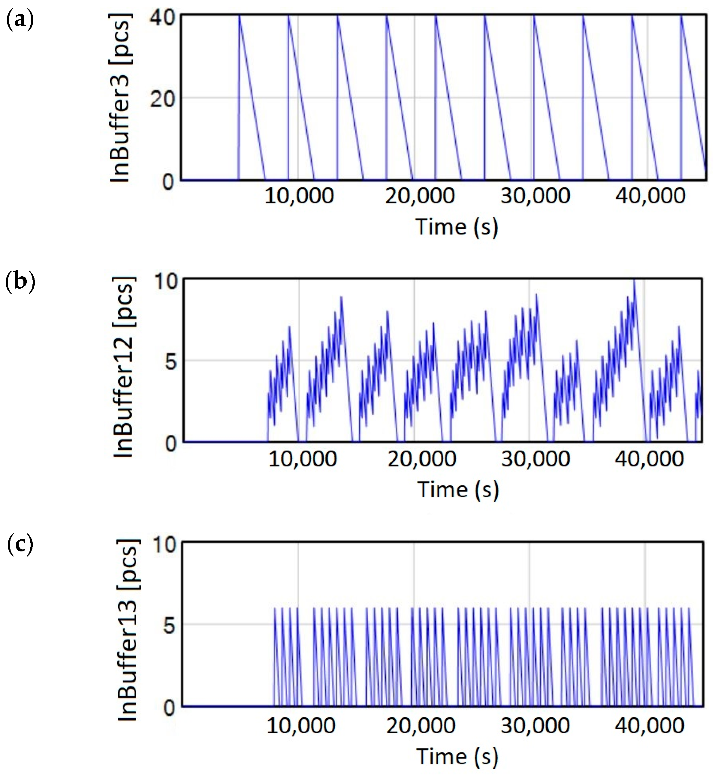
4.2. Identification and Elimination of Bottlenecks in the Brake Caliper Body Remanufacturing Process

The analysis of the results of the conducted simulation experiments also showed the accumulation of excessive stocks (exceeding the size of the transport batch) in the input trays of the selected processes. The inventory level of the input trays of processes P3, P12, and P13. The data shown in the graphs (Figure 9) indicate the accumulation of excessive inventory in the InBuffer3, InBuffer12, and, to a smaller extent, InBuffer13 storage bins.
A solution to this problem was proposed by increasing the number of employees at P3-sorting and P12-assembly stations to two. This modification led to an increase in the efficiency of the P3 and P12 processes, as a result of the intensity of the accumulation of excessive stocks in the InBuffer13 (Figure 10).
The problem was solved by doubling the staffing and, thus, the throughput of the P13 process. The modifications carried out eliminated the excessive inventory of work-in-progress (Figure 11).
The increase in staffing has reduced the maximum stock levels in the InBuffer3, Inbuffer12, and Inbuffer13 storage bins. This is particularly evident for InBuffer12, where the maximum stock level was reduced from more than 100 to 10 units. The considerations presented here indicate that increasing the manning of the P12 process makes the greatest contribution to reducing work-in-progress inventory and should be a priority action in balancing the production line under consideration. Increasing the staffing also resulted in a reduction in customer lead time, as discussed in Section 4.3.

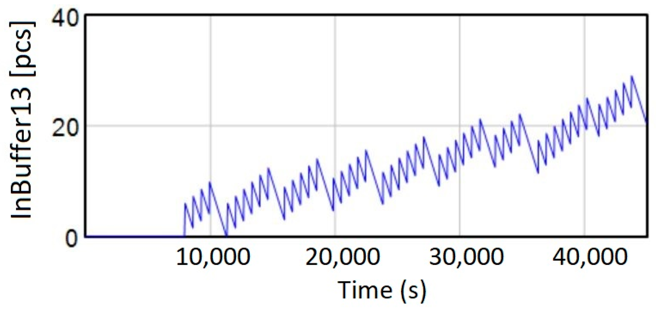
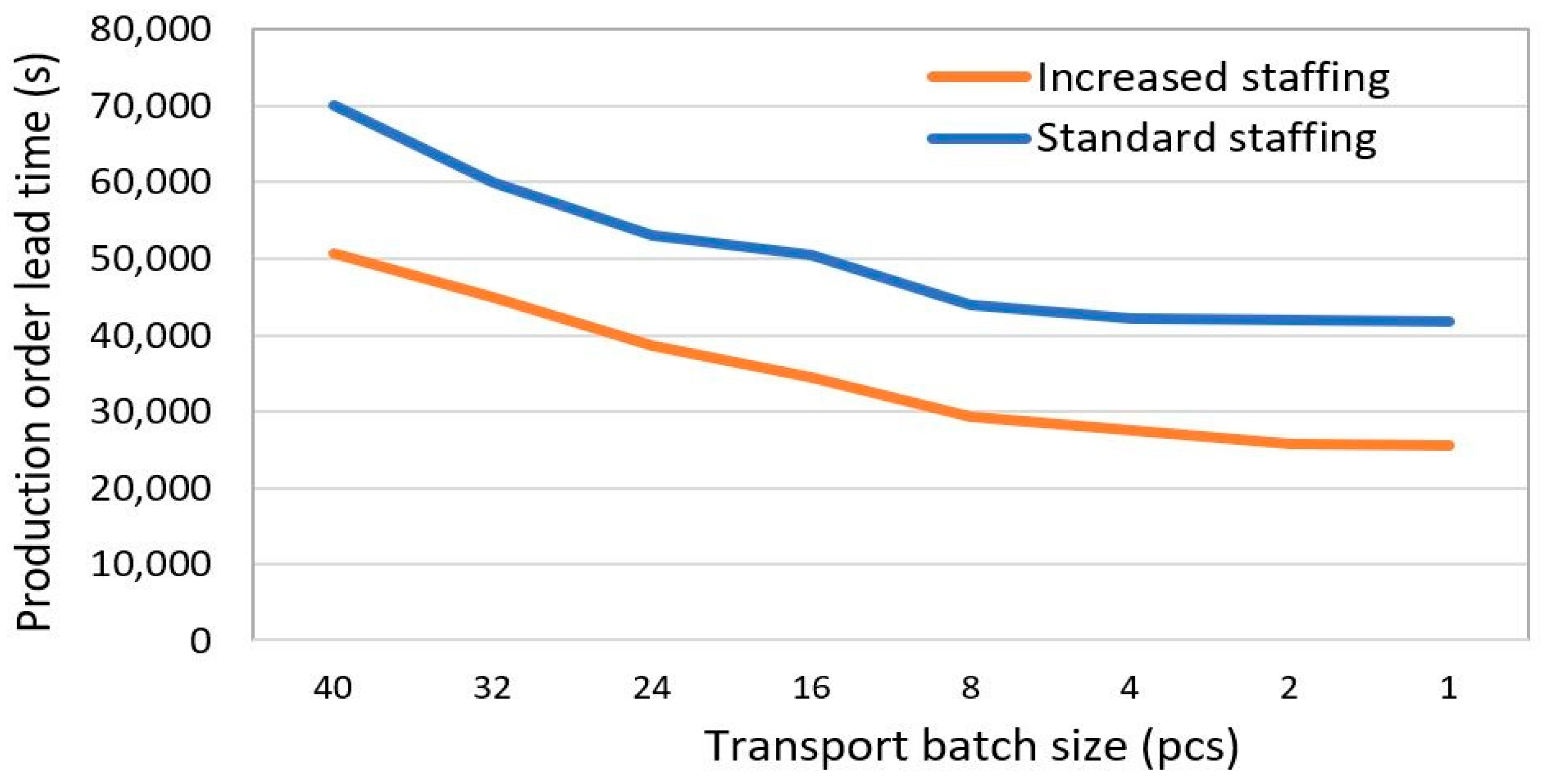
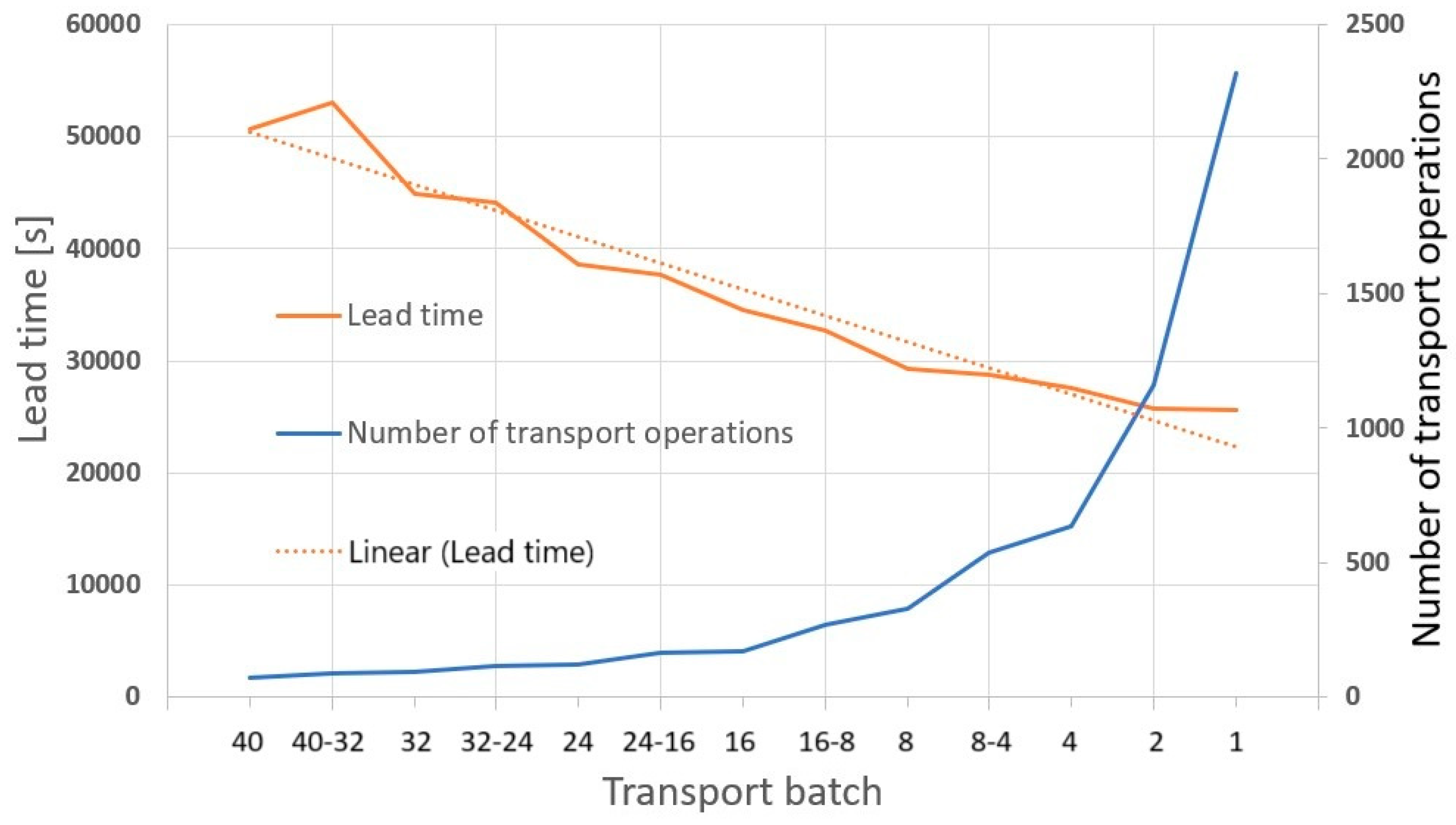
4.3. Determination of the Optimal Size of the Transport Batch

In the next stage of the research, a study of lead times was conducted for different transport lot sizes. It should be noted that in the process in question, maintaining a constant batch size for all transport operations is hampered by a large percentage of waste and different operation sequences for particular brake caliper bodies. Therefore, only a “reference” transport batch size was determined and transport volumes between operations were calculated based on it. If, for example, a batch of 40 pieces is sent to the sorting operation, on average 6 pieces are waste, 7 pieces are transported to the cutting operation, and 27 pieces are sent to the CNC machining station. For example, after the sorting operation, 15% of the bodies constitute production waste, 17% are sent to the cutting operation, and the remaining 68% are sent directly to the CNC station. The model of transport batch distribution after the sorting operation (P3) includes 3 flows: T3, PZ3, and TOIB5 (Figure 12), representing the movement of items, respectively, to the input tray of the process P4, the waste storage bin after the sorting process Z3, and the input tray of the process P5.
Flows T3, PZ3, and TOIB5 are given by Equations (1)–(3):
TOIB5 = IF THEN ELSE(OutBuffer3 >= TB3, TB3, 0) × 0.68
PZ3 = IF THEN ELSE(OutBuffer3 >= TB3, TB3, 0) × 0.15
T3 = IF THEN ELSE(OutBuffer3 >= TB3, TB3, 0) × 0.17
where: OutBuffer3—stock level of the OutBuffer3 and TB3—transport batch size after P3 operation.
Table 4 and Table 5 show the turnaround time of production orders for different transport batch sizes for standard and increased production process staffing.
The data presented in Table 5 show that the increase in manning resulted in a significant reduction in order processing time. For example, for a shipment batch of 40 units, the fulfillment of an order of 160 clamps requires 69,992 (s) (19.4 h), and after increasing the staffing, the same order is completed in 50,622 (s) (14.06 h). It is worth noting that increasing the staffing of stations P3, P12, and P13 (sorting, assembly, and leak test) does not require the purchase of machine tools or other expensive equipment.
The results of the conducted experiments also indicate that the execution time of an order decreases as the size of the transport batch decreases (Figure 13). This is possible when transport operations are carried out without interrupting technological operations, for example, with the use of automatic transport equipment, additional workers carrying out transport operations, or transport during the operation of an unmanned machine tool.
Reducing the size of the transport batch results in a reduction of the production order lead time (Figure 13) for both standard and increased staffing. In the following numerical simulation experiments, the number of transport operations was determined for the fulfillment of an order to remanufacture 160 brake calipers (Table 6).
The results in Table 4 and Table 5 show that shortening the order fulfillment time is possible by reducing the size of the transport batch. On the other hand, reducing the size of the transport batch increases the number of transport operations, which involve additional work and costs.
The possibility of using two “reference” transport batch sizes in transport operations was also examined. In this study, the principle was adopted that smaller transport batches are transferred from shorter operations to longer ones, and larger transport batches are transferred from longer operations to shorter ones. The number of transport operations for the fulfillment of the order for the remanufacturing of 160 brake calipers with the adopted transport batch size: 40, 32, 24, 16, 8, 4, 2, and 1 pc, as well as for the production based on two transport batch sizes (40–32, 32–24, 24–16, 16–8, and 8–4) are shown in Table 7.
The results in Table 7 indicate the low usefulness of constructing routes with two transport batch sizes, especially for large batch sizes. For example, if we consider the introduction of a production flow based on two transport batch sizes 40–32 instead of a flow with a batch size of 40, we will obtain an extension of the order execution time from 50,622 s to 52,779 s and an increase in the number of transport operations from 75 to 87. At the same time, the use of a transport batch with a size of 32 pieces will allow for a shorter order execution time (44,890 s) with a slightly larger (96) number of transport operations. As the size of the transport batch decreases, the benefits of using transport based on two transport batch sizes become visible, e.g., 24–16, 16–8, and 8–4. Thanks to this, we obtain an intermediate lead time and an intermediate number of transport operations—which give greater opportunities to adapt to the customer order schedule. It is also worth noting that a significant reduction in the size of the transport batch (even to the flow of a single item) results in a slight reduction in the order fulfillment time, with a rapidly increasing number of transport operations (Figure 14).

5. Summary and Conclusions

The article presents the issue of optimizing the flow of parts in the process of remanufacturing brake calipers. Attention was paid to the specificity and complexity of the regeneration process as well as the complexity of the problem of predicting waste/scrapping of brake caliper bodies in individual operations.
During the analysis of the production process (using computer simulation methods), bottlenecks were identified and solutions were proposed to eliminate them. The provided experiments carried out allowed the following conclusions to be formulated:
  • The introduction of a reduced transport batch size seems to be a key element of optimizing the production process. Experiments confirm that shortening the order fulfillment time is possible by using transport operations that do not require interruption of technological operations;
  • Automatic transport devices, or transport during the operation of the machine tool that does not require maintenance, are potential solutions aimed at increasing the smoothness and efficiency of the regeneration process;
  • A significant reduction in the size of the transport batch, even down to the flow of a single item, may result in a slight reduction in the order processing time, with a simultaneous sharp increase in the number of transport operations (the optimal size of the transport batch should, therefore, be carefully selected, taking into account various factors such as the type of operation, staffing, and the efficiency and cost of transportation operations).

Author Contributions

Conceptualization, P.L., A.G. and Ł.W.; methodology, P.L. and A.G.; software, P.L.; validation, A.G.; formal analysis, Ł.W. and M.C.; investigation, P.L. and A.G.; resources, Ł.W.; data curation, Ł.W.; writing—original draft preparation, P.L. and Ł.W.; writing—review and editing, A.G.; visualization, P.L., A.G. and Ł.W.; supervision, A.G. and M.C.; project administration, A.G.; funding acquisition, A.G. All authors have read and agreed to the published version of the manuscript.

Funding

The research leading to these results has received funding from the commissioned task entitled “VIA CARPATIA Universities of Technology Network named after the President of the Republic of Poland Lech Kaczyński”, contract no. MEiN/2022/DPI/2578, and action titled “In the neighborhood—inter-university research internships and study visits”.

Data Availability Statement

Data are contained within the article.

Conflicts of Interest

The authors declare no conflict of interest.

References

  1. Qi, R.; Khan, A.J.; Basheer, M.F.; Hameed, W.U.; Chaudhry, I.S. Resolving the resource curse through effective utilization of available natural resources and claiming sustainable development. Resour. Policy 2023, 87, 104285. [Google Scholar] [CrossRef]
  2. Hofmann, M.; Hofmann, H.; Hageluken, C.; Hool, A. Critical raw materials: A perspective from the materials science community. Sustain. Mater. Technol. 2018, 17, e00074. [Google Scholar] [CrossRef]
  3. Mallik, A.K. The future of the technology-based manufacturing in the European Union. Results Eng. 2023, 19, 101356. [Google Scholar] [CrossRef]
  4. Świć, A.; Gola, A. Economic analysis of casing parts production in a flexible manufacturing system. Actual Probl. Econ. 2013, 141, 526–533. [Google Scholar]
  5. Domenech, T.; Borrion, A. Embedding Circular Economy Principles into Urban Regeneration and Waste Management: Framework and Metrics. Sustainability 2022, 14, 1293. [Google Scholar] [CrossRef]
  6. Alhawari, O.; Awan, U.; Bhutta, M.K.S.; Ülkü, M.A. Insights from Circular Economy Literature: A Review of Extant Definitions and Unravelling Paths to Future Research. Sustainability 2021, 13, 859. [Google Scholar] [CrossRef]
  7. De Pascale, A.; Vita, G.D.; Giannetto, C.; Ioppolo, G.; Lanfranchi, M.; Limosani, M.; Szopik-Depczyńska, K. The circular economy implementation at the European Univion level. Past, present and future. J. Clean. Prod. 2023, 423, 138658. [Google Scholar] [CrossRef]
  8. Napoleone, A.; Bruzzone, A.; Andersen, A.-L.; Brunoe, T.D. Fostering the reuse of manufacuturing resources for resilient and sustainable supply chains. Sustainability 2022, 14, 5890. [Google Scholar] [CrossRef]
  9. Power, J.M.; Ou-Yang, C.; Juan, Y.-C. Optimize batch size combination using improved hybrid particle swarm optimization. Procedia Comput. Sci. 2022, 197, 370–376. [Google Scholar] [CrossRef]
  10. Kin, S.T.M.; Ong, S.K.; Nee, A.Y.C. Remanufacutring process planning. Procedia CIRP 2014, 15, 189–194. [Google Scholar] [CrossRef]
  11. Ke, C.; Jiang, Z.; Zhu, S.; Wang, Y. An integrated design method for remanufacturing processes based on performance demand. Int. J. Adv. Manuf. 2022, 118, 849–863. [Google Scholar] [CrossRef]
  12. Wójcik, Ł.; Gola, A. Working time standardization in the assembly process of regenerated elements using MES system and timing method. Lect. Notes Netw. Syst. 2023, 741, 46–55. [Google Scholar]
  13. Silva Teixeira, E.L.; Tjahjono, B.; Beltran, M.; Juliao, J. Demystifying the digital transition of remanufacturing: A systematic review of literature. Comput. Ind. 2022, 134, 103567. [Google Scholar] [CrossRef]
  14. Plinta, D.; Radwan, K. Improving material flow in a modified production system. Appl. Comput. Sci. 2023, 19, 95–106. [Google Scholar] [CrossRef]
  15. Kuthambalayan, T.S.; Bera, S. Managing product variety with mixed make-to-stock/make to order production strategy and guaranteed delivery time under stochastic demand. Comput. Ind. Eng. 2020, 147, 106603. [Google Scholar] [CrossRef]
  16. Soman, C.A.; van Donk, D.P.; Gaalman, G. Combined make-to-order and make-to-stock in a food production system. Int. J. Prod. Econ. 2004, 90, 223–235. [Google Scholar] [CrossRef]
  17. Synnes, E.L.; Welo, T. Bridging the gap between high and low-volume production through enhancement of integrative capabilities. Procedia Manuf. 2016, 5, 26–40. [Google Scholar] [CrossRef]
  18. Gan, Z.L.; Musa, S.N.; Yap, H.J. A review of the high-mix, low-volume manufacturing industry. Appl. Sci. 2023, 13, 1687. [Google Scholar] [CrossRef]
  19. Danilczuk, W.; Gola, A.; Grznar, P. Job scheduling algorithm for a hybrid MTO-MTS production process. IFAC Pap. 2022, 55, 451–456. [Google Scholar] [CrossRef]
  20. Yano, S.; Nagasawa, K.; Morikawa, K.; Takahashi, K. A dynamic switching policy with thresholds of inventory level and waiting orders for MTS/MTO hybrid production systems. Procedia Manuf. 2019, 39, 1076–1081. [Google Scholar] [CrossRef]
  21. Peeters, K.; van Ooijen, H. Hybrid make-to-stock and make-to-order systems: A taxonomic review. Int. J. Prod. Res. 2020, 58, 4659–4688. [Google Scholar] [CrossRef]
  22. Kang, Z.; Catal, C.; Tekinerdogan, B. Product failure detection for production lines using a data-driven model. Expert Syst. Appl. 2022, 202, 117398. [Google Scholar] [CrossRef]
  23. Derhab, N.; Elkhwesky, Z. A systematic and critical review of waste management in micro, small and medium-sized enterprises: Future directions for theory and practice. Environ. Sci. Pollut. Res. 2023, 30, 13920–13944. [Google Scholar] [CrossRef] [PubMed]
  24. Brzozowska, J.; Pizoń, J.; Baytikenova, G.; Gola, A.; Zakimova, A.; Piotrowska, K. Data engineering in CRISP-DM process production data—Case study. Appl. Comput. Sci. 2023, 19, 83–95. [Google Scholar] [CrossRef]
  25. Wei, H.; Yuan, J.; Gao, Y. Transportation and batching scheduling for minimizing total weighted completion time. Mathematics 2019, 7, 819. [Google Scholar] [CrossRef]
  26. Zhu, H. A two stage scheduling with transportation and batching. Inf. Process. Lett. 2012, 112, 728–731. [Google Scholar] [CrossRef]
  27. Schoenberger, L.; Schmid, A.; Tanase, R.; Beck, M.; Schwaninger, M. Structural analysis of system dynamics models. Simul. Model. Pract. Theory 2021, 110, 102333. [Google Scholar] [CrossRef]
  28. Sterman, J.D. Business Dynamics: Systems Thinking and Modeling for a Complex World; McGraw-Hill: Boston, MA, USA, 2000. [Google Scholar]
  29. Senge, P.M. Piąta Dyscyplina: Teoria i Praktyka Organizacji Uczących Się; Oficyna Wolters Kluwer Business: Warsaw, Poland, 2012. (In Polish) [Google Scholar]
  30. Forrester, J.W. Industrial Dynamics; MIT Press: Cambridge, MA, USA, 1961. [Google Scholar]
  31. Morecroft, J.D.W.; Sterman, J.D. Modelling for Learning Organizations; Productivity Press: Portland, OR, USA, 1994. [Google Scholar]
  32. Mourtzis, D.; Doukas, M.; Bernidaki, D. Simulation in manufacturing: Review and challenges. Procedia CIRP 2014, 25, 213–229. [Google Scholar] [CrossRef]
  33. De Paula Ferreira, W.; Armellini, F.; de Santa-Eulalia, L.A. Simulation in Industry 4.0: A state-of-the-art review. Comput. Ind. Eng. 2020, 149, 106868. [Google Scholar] [CrossRef]
  34. De Sousa Junior, W.T.; Montevechi, J.A.B.; De Carvalho, M.R.; Campos, A.T. Discrete simulation-based optimization methods for industrial engineering problems: A systematic literature review. Comput. Ind. Eng. 2019, 128, 526–540. [Google Scholar] [CrossRef]
  35. EFFRA—Factories of the Future-Multi-Annual Roadmap for the Contractual PPP under Horizon. 2000. Available online: https://www.effra.eu/sites/default/files/factories_of_the_future_2020_roadmap.pdf (accessed on 18 September 2023).
  36. Lu, Y.; Morris, K.C.; Frechette, S. Current standards landscape for smart manufacturing systems. Natl. Inst. Stand. Technol. 2016, 39, 8107. [Google Scholar]
  37. Monostori, L.; Váncza, J.; Kumara, S.R. Agent-based systems for manufacturing. CIRP Ann. 2006, 55, 697–720. [Google Scholar] [CrossRef]
  38. Jahangirian, M.; Eldabi, T.; Naseer, A.; Stergioulas, L.K.; Young, T. Simulation in manufacturing and business: A review. Eur. J. Oper. Res. 2010, 203, 1–13. [Google Scholar] [CrossRef]
  39. Morgan, J.S.; Howick, S.; Belton, V. A toolkit of designs for mixing discrete event simulation and System Dynamics. Eur. J. Oper. Res. 2017, 257, 907–918. [Google Scholar] [CrossRef]
  40. Linnéusson, G.; Ng, A.H.; Aslam, T. A hybrid simulation-based optimization framework supporting strategic maintenance development to improve production performance. Eur. J. Oper. Res. 2020, 281, 402–414. [Google Scholar] [CrossRef]
  41. Litwin, P.; Antonelli, D.; Stadnicka, D. Disabled employees on the manufacturing line: Simulations of impact on performance and benefits for companies. IFAC Pap. 2022, 55, 848–853. [Google Scholar] [CrossRef]
  42. Oleghe, O.; Salonitis, K. Hybrid simulation modelling of the human-production process interface in lean manufacturing systems. Int. J. Lean Six Sigma 2019, 10, 665–690. [Google Scholar] [CrossRef]
  43. Roci, M.; Salehi, N.; Amir, S.; Shoaib-ul-Hasan, S.; Asif, F.M.; Mihelič, A.; Rashid, A. Towards circular manufacturing systems implementation: A complex adaptive systems perspective using modelling and simulation as a quantitative analysis tool. Sustain. Prod. Consum. 2022, 31, 97–112. [Google Scholar] [CrossRef]
  44. Adane, T.F.; Nicolescu, M. Towards a generic framework for the performance evaluation of manufacturing strategy: An innovative approach. J. Manuf. Mater. Process. 2018, 2, 23. [Google Scholar] [CrossRef]
  45. Guizzi, G.; Miele, D.; Santillo, L.C.; Romano, E. A System Dynamics approach for the operational control of production. In Proceedings of the 2013 IEEE 12th International Conference on Intelligent Software Methodologies, Tools and Techniques (SoMeT), Budapest, Hungary, 22–24 September 2013; pp. 69–74. [Google Scholar] [CrossRef]
  46. Stadnicka, D.; Litwin, P. Value stream mapping and system dynamics integration for manufacturing line modelling and analysis. Int. J. Prod. Econ. 2019, 208, 400–411. [Google Scholar] [CrossRef]
  47. Stadnicka, D.; Litwin, P. Problems of System Dynamics model development for complex product manufacturing process. J. Phys. Conf. Ser. 2022, 2198, 012062. [Google Scholar] [CrossRef]
  48. Yang, H.; Bukkapatnam, S.T.; Barajas, L.G. Continuous flow modelling of multistage assembly line system dynamics. Int. J. Comput. Integr. Manuf. 2013, 26, 401–411. [Google Scholar] [CrossRef]
Figure 2. Brake caliper body: (a) before the regeneration process and (b) after the regeneration process.
Processes 12 00016 g002
Figure 3. Regeneration scheme of brake calipers.
Processes 12 00016 g003
Figure 4. Average amounts of waste at each stage of the regeneration process.
Processes 12 00016 g004
Figure 5. Transport containers used in the process of remanufacturing brake caliper bodies.
Processes 12 00016 g005
Figure 6. Transport equipment used in the process of remanufacturing brake caliper bodies: (a) roller conveyor and (b) scissor transport cart.
Processes 12 00016 g006
Figure 7. Structure diagram of the production workstation model.
Processes 12 00016 g007
Figure 8. Remanufacturing process of brake caliper body model.
Processes 12 00016 g008
Figure 9. Stock levels during simulation—standard staffing: (a) InBuffer3, (b) InBuffer12, and (c) InBuffer13.
Processes 12 00016 g009
Figure 10. InBuffer13 level with increased P3 and P12 staffing.
Processes 12 00016 g010
Figure 11. Stock levels during simulation—increased staffing: (a) InBuffer3, (b) InBuffer12, and (c) InBuffer13.
Processes 12 00016 g011
Figure 12. Diagram of the distribution of a batch after a sorting operation (P3).
Processes 12 00016 g012
Figure 13. Production order lead time (160 pcs) for different batch sizes with standard and increased staffing.
Processes 12 00016 g013
Figure 14. Production order lead time and number of transport operations for different batch sizes (increased staffing).
Processes 12 00016 g014
Table 1. Average unit time of technological operations.
SymbolName of the Technological OperationAverage Unit Time (s)
P1Disassembly104
P2Washing672 *
P3Sort and verification110
P4Surface regeneration93
P5Thread regeneration33
P6CNC milling189
P7Quality control89
P8Applying the putty222
P9Cleaning37
P10Assembly of the sleeve72
P11Parts collection55
P12Assembly215
P13Final test80
* Washing time of batches of up to 40 pieces.
Table 2. Average unit time of transport operations.
SymbolAverage Unit Time (s)SymbolAverage Unit Time (s)
T154T712
T266ToIB917
T312T821
ToIB522T99
T49T1011
T514T1110
T620T1212
ToIB718T1358
Table 3. The waste level in the completion of a production order.
Order
Size (pcs)
Scraps Level (pcs)
Z3Z4Z6Z7Z13Total *
8015.150.341.440.830.7921
12022.950.522.181.261.231
160300.682.861.651.638
* The total waste level was determined after rounding up to the total of the individual storage units.
Table 4. Production order lead time—standard staffing.
Order SizeTransport Batch/Production Order Lead Time (s)
403224168421
8051,41342,90235,23433,26726,65324,37623,61623,551
12059,46450,49144,77241,88135,34633,35332,84032,725
16069,99260,08052,99050,49643,96742,08841,97641,784
Table 5. Production order lead time—increased staffing.
Order SizeTransport Batch/Production Order Lead Time (s)
403224168421
8039,05631,41025,65523,52318,51116,46015,32115,161
12043,89635,85132,56828,42923,93121,47420,34720,119
16050,62244,89038,57134,51029,36027,56325,72525,570
Table 6. Number of transport operations for different transport batches.
Transport Batch403224168421
Number of transport
operations
759612317233163711632320
Table 7. Lead time and number of transport operations for different transport batches.
Transport Batch4040–323232–242424–161616–888–4421
Number of transport
operations
75879611512316517226833153563711632320
Lead time50,62252,99744,89044,16338,57137,75634,51032,69529,36028,75727,56325,72525,570
Disclaimer/Publisher’s Note: The statements, opinions and data contained in all publications are solely those of the individual author(s) and contributor(s) and not of MDPI and/or the editor(s). MDPI and/or the editor(s) disclaim responsibility for any injury to people or property resulting from any ideas, methods, instructions or products referred to in the content.

