
Research and Test on the Device of Downhole Near-Bit Temperature and Pressure Measurement While Drilling
Abstract
:1. Introduction
2. Design for High-Temperature Measurement While Drilling
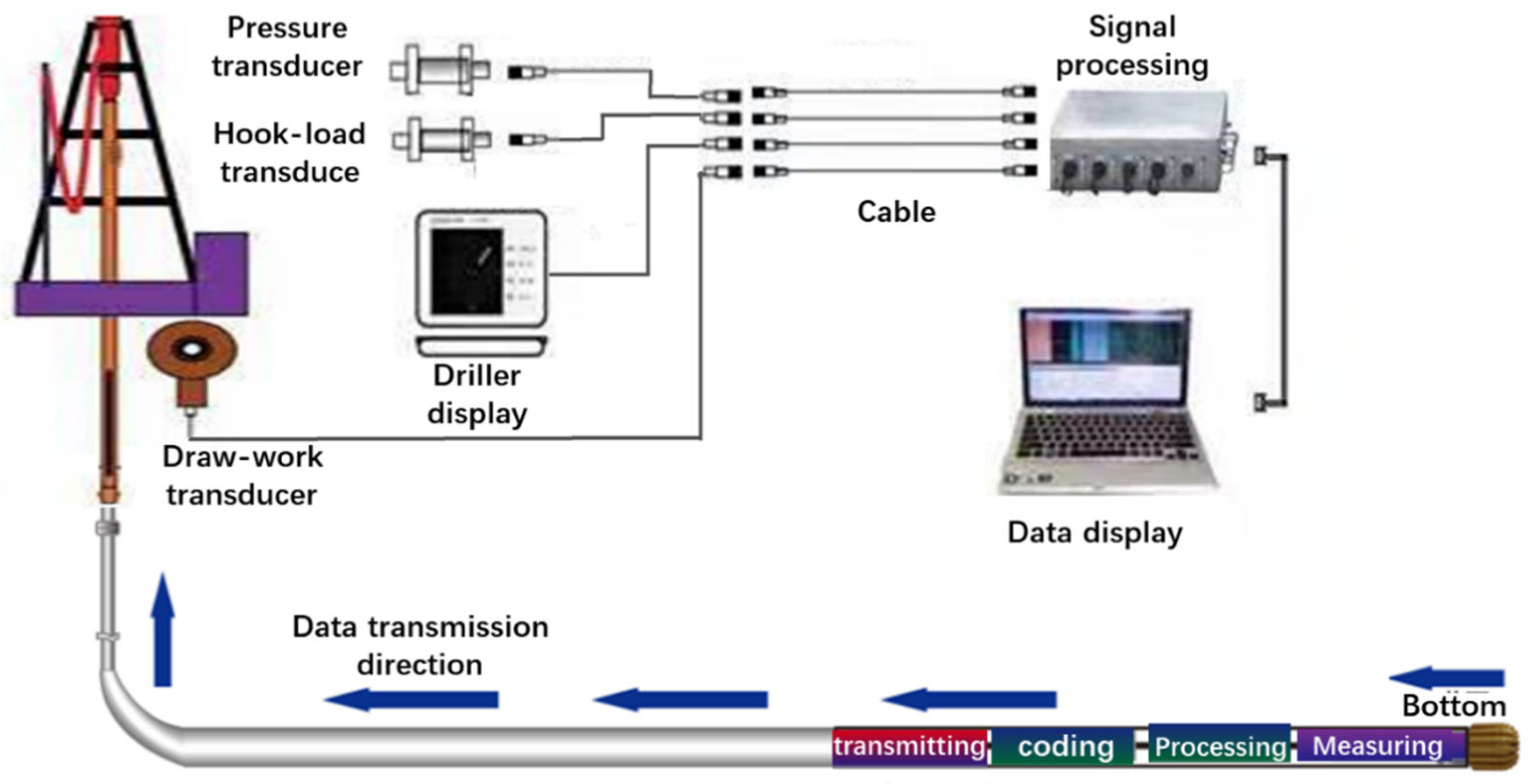
2.1. Measurement Composition
2.2. Working Principle of Measurement System
3. Key Technologies of Measurement Devices
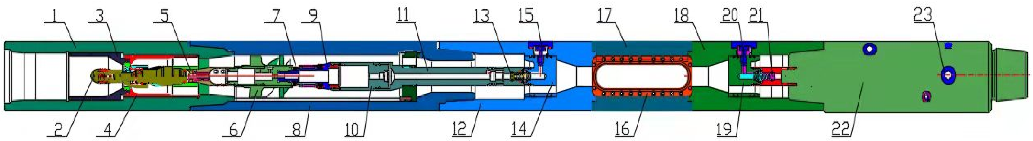
3.1. Mechanical Design
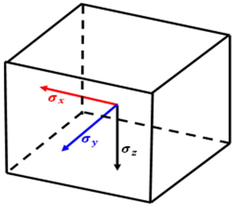
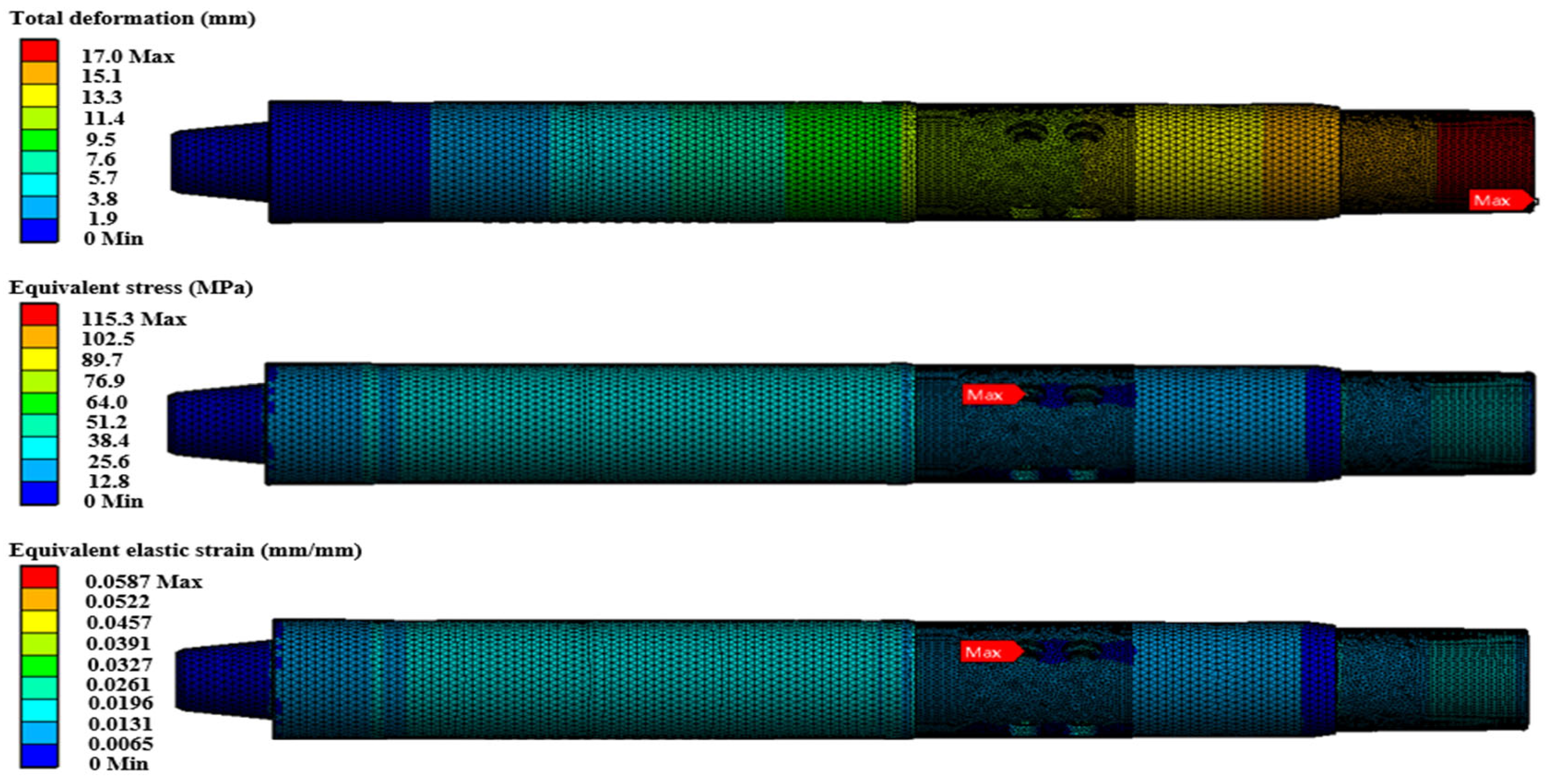
3.2. Strength Check
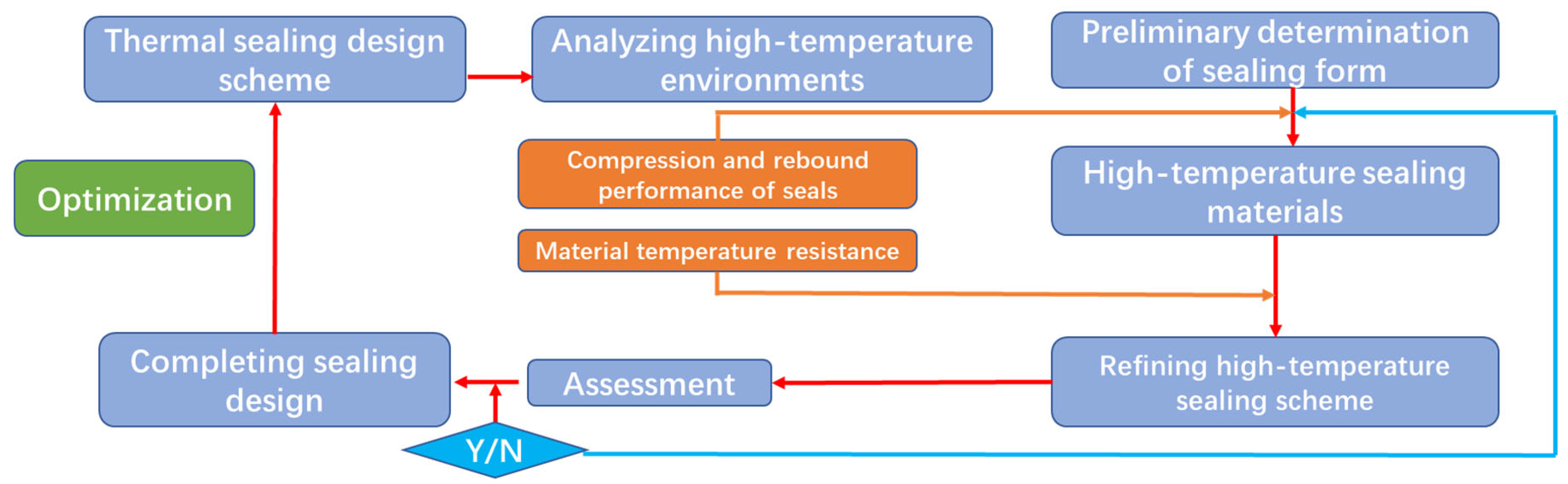
3.3. Seal Design
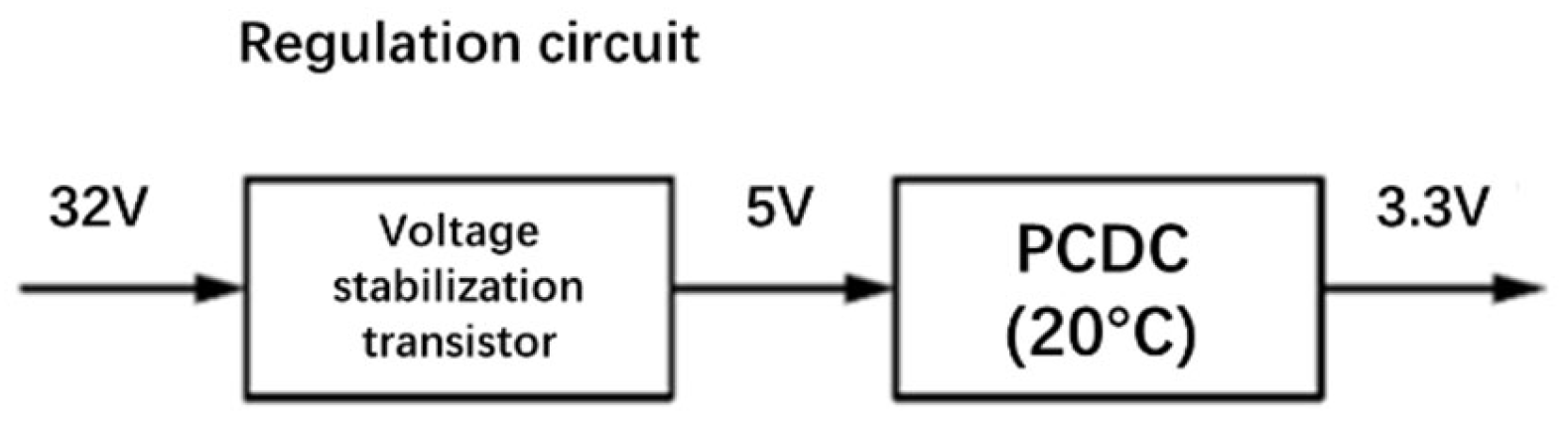
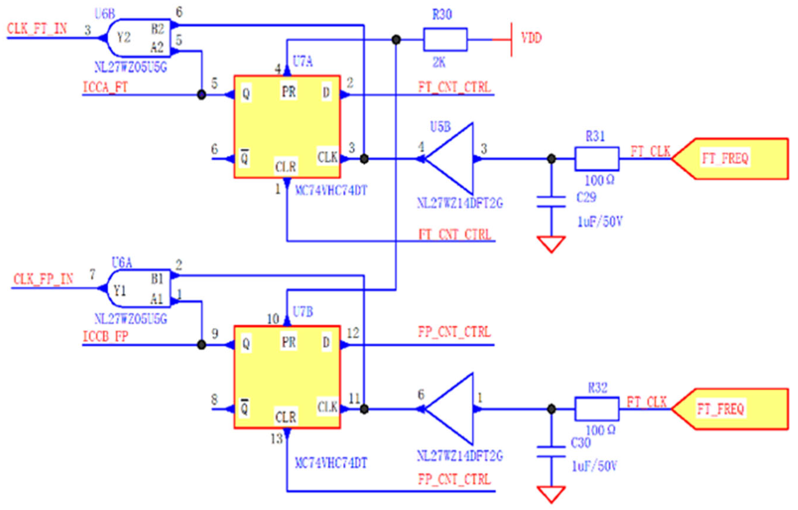
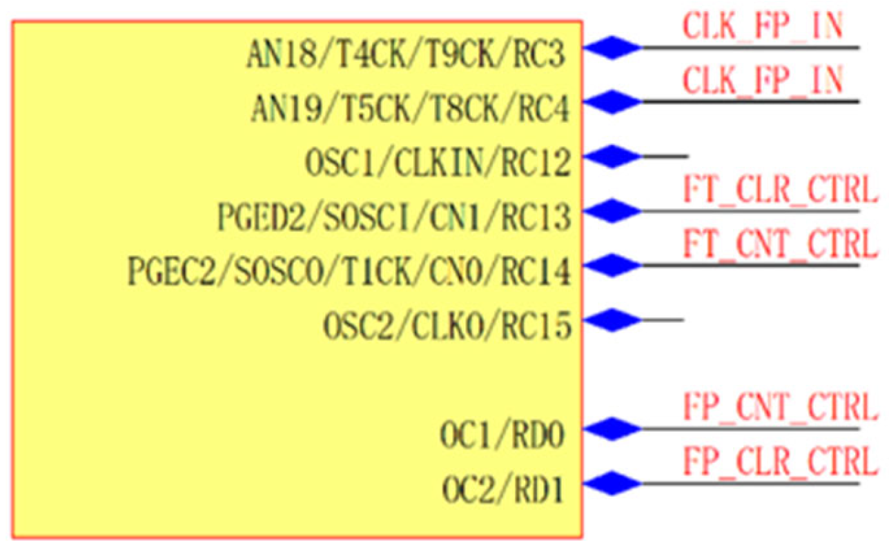
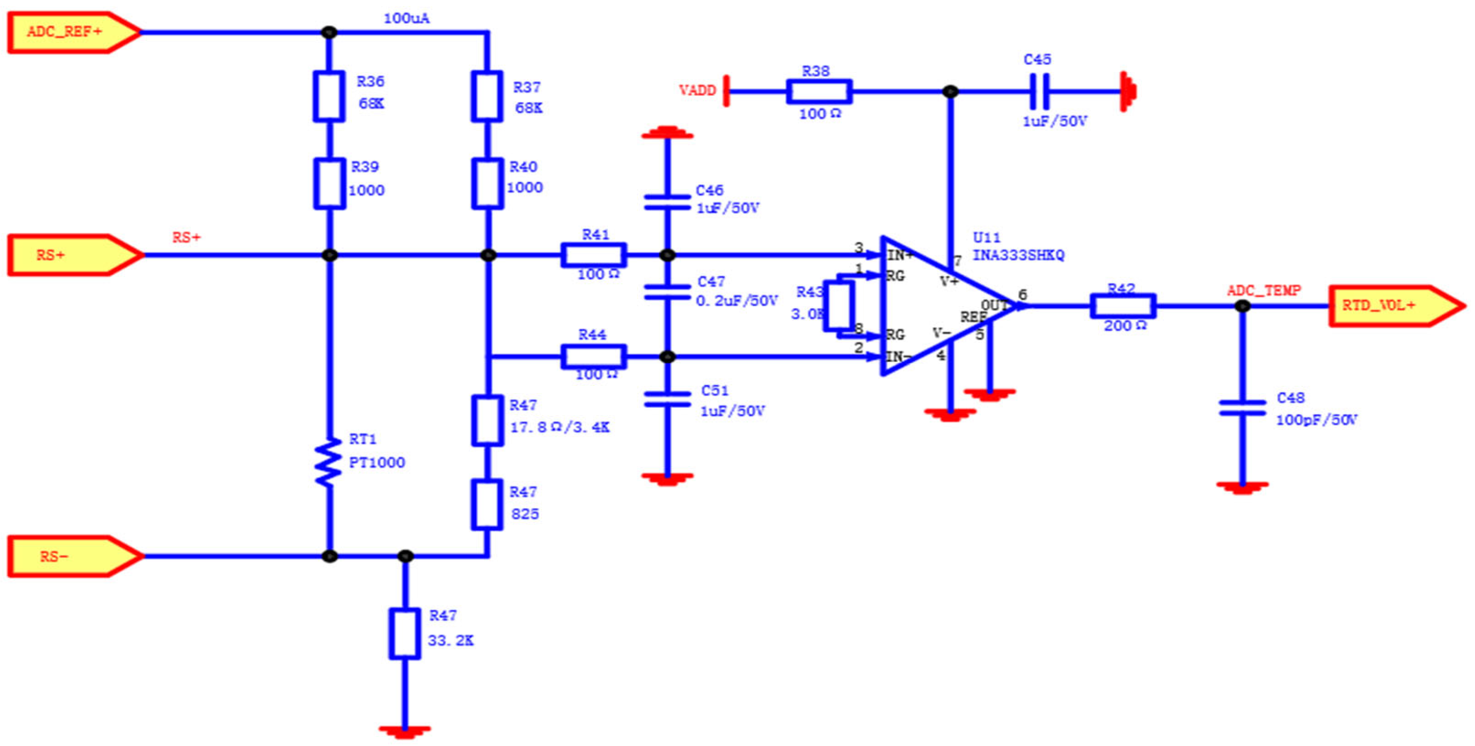
3.4. Design of Temperature and Pressure Measurement Circuit
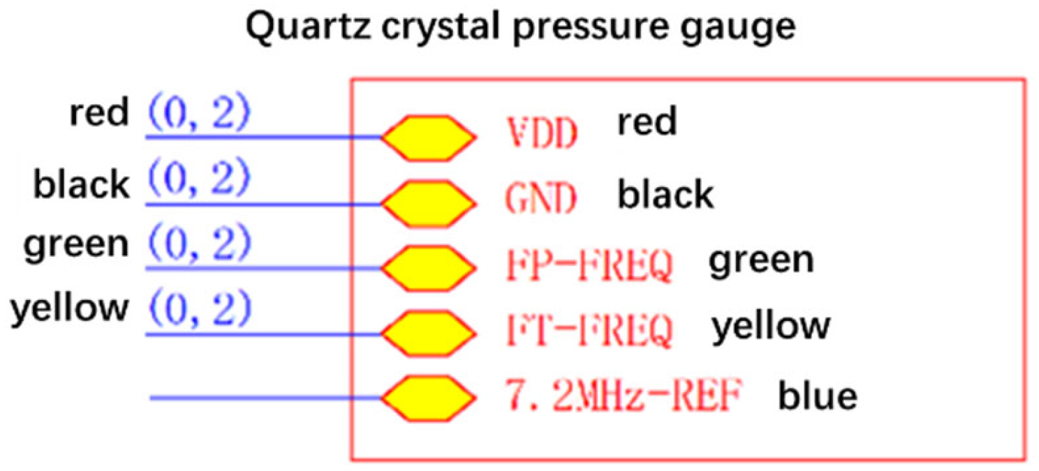
3.5. Selection of Pressure Sensors
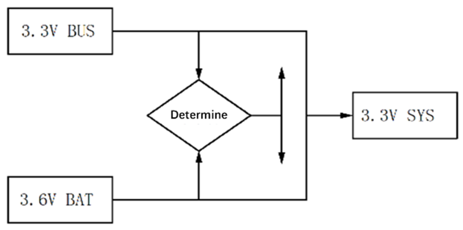
3.6. Data Transmission Module
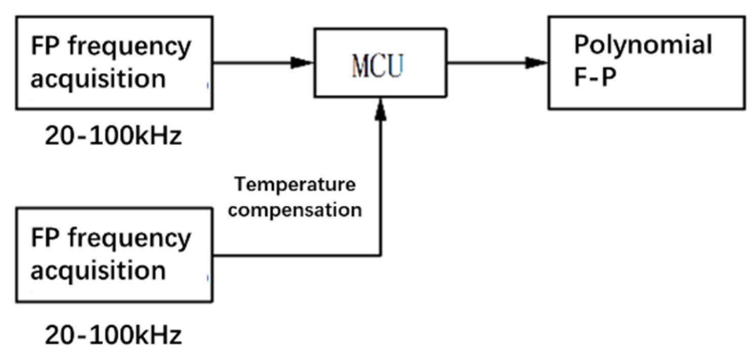
3.7. Signal Processing Methodology
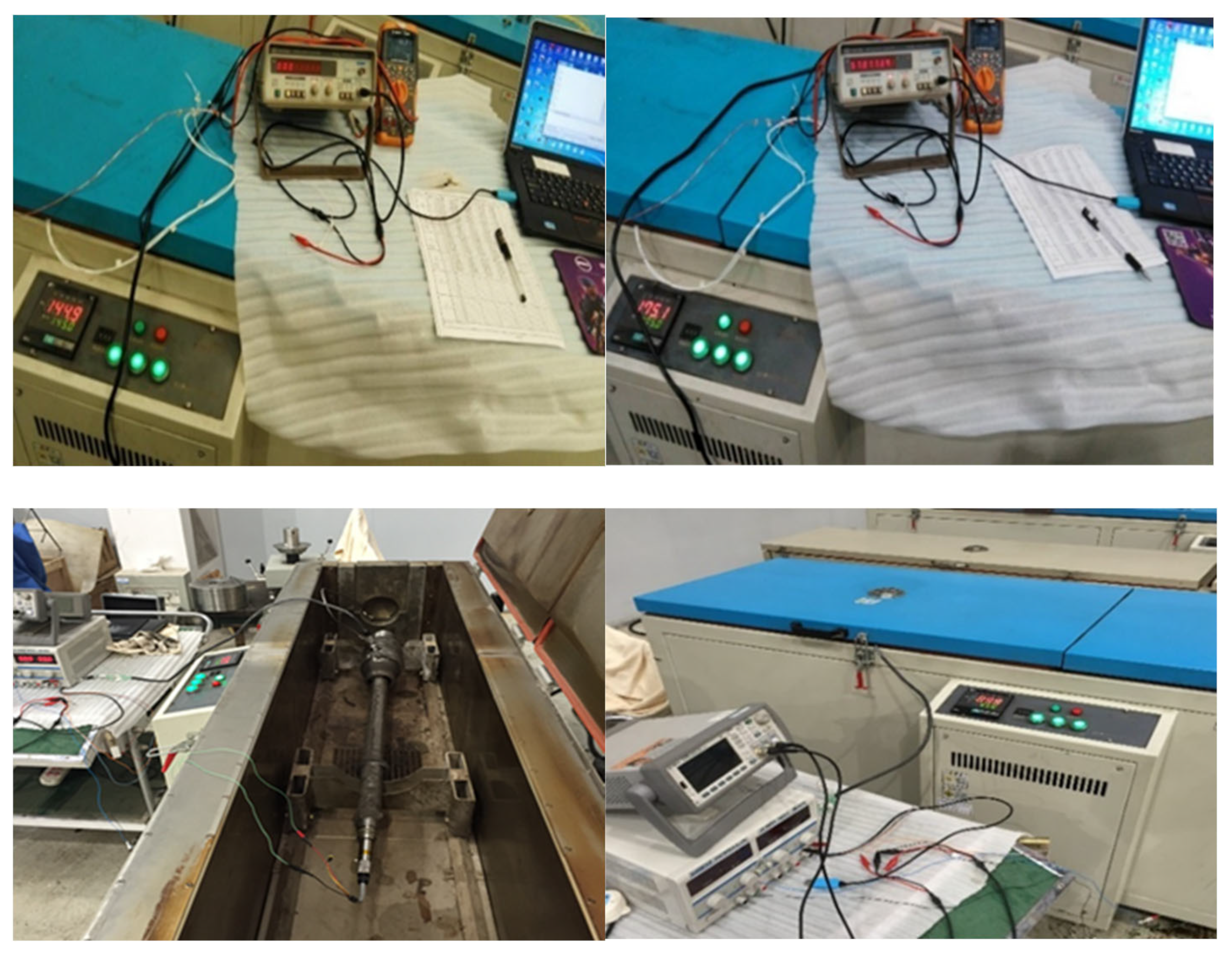
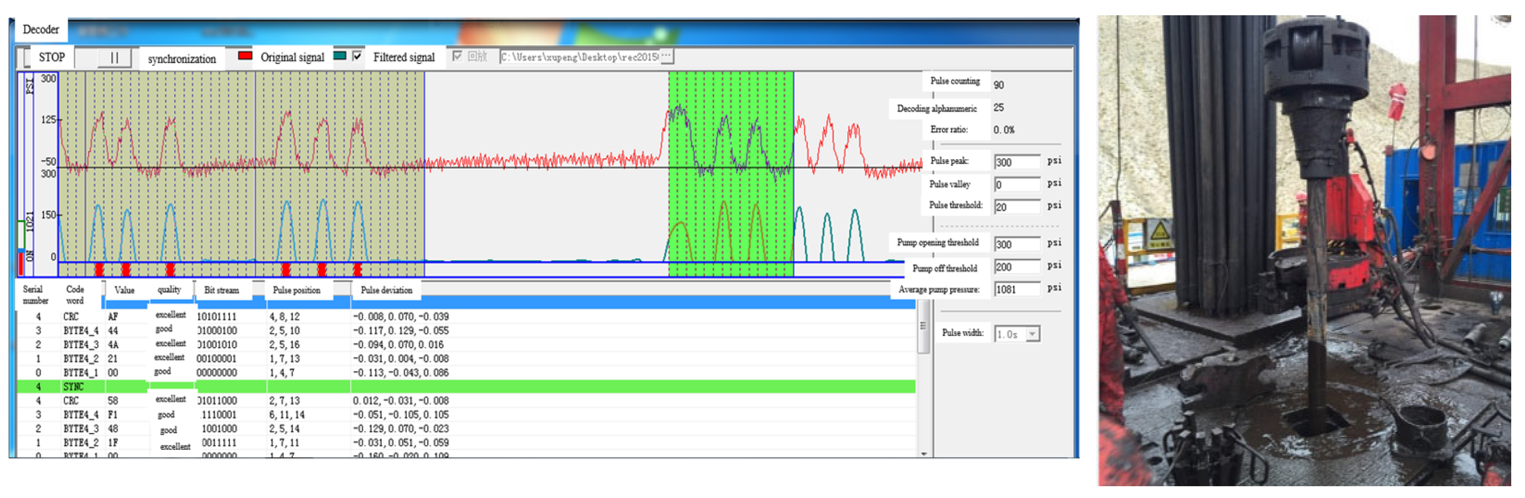
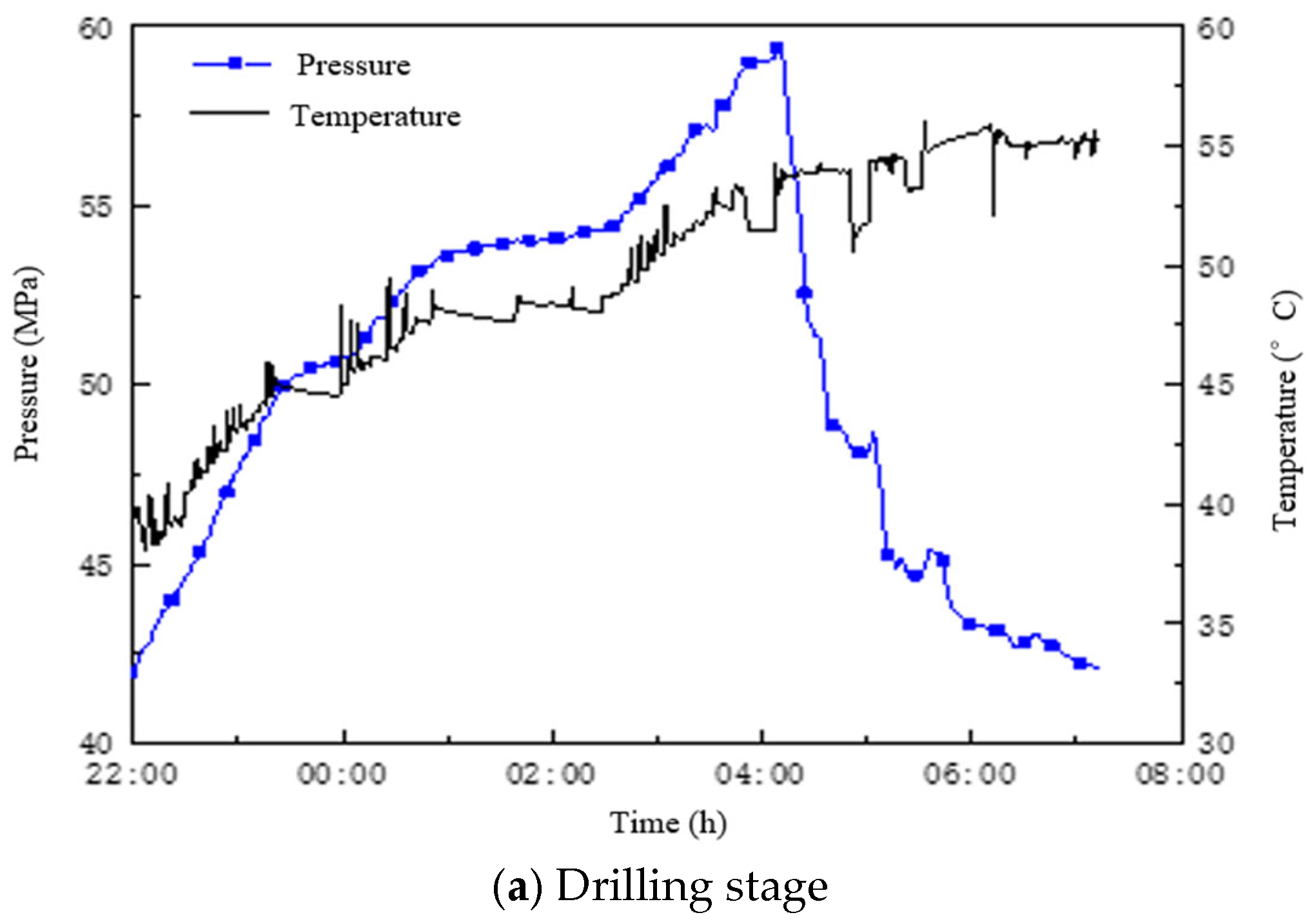
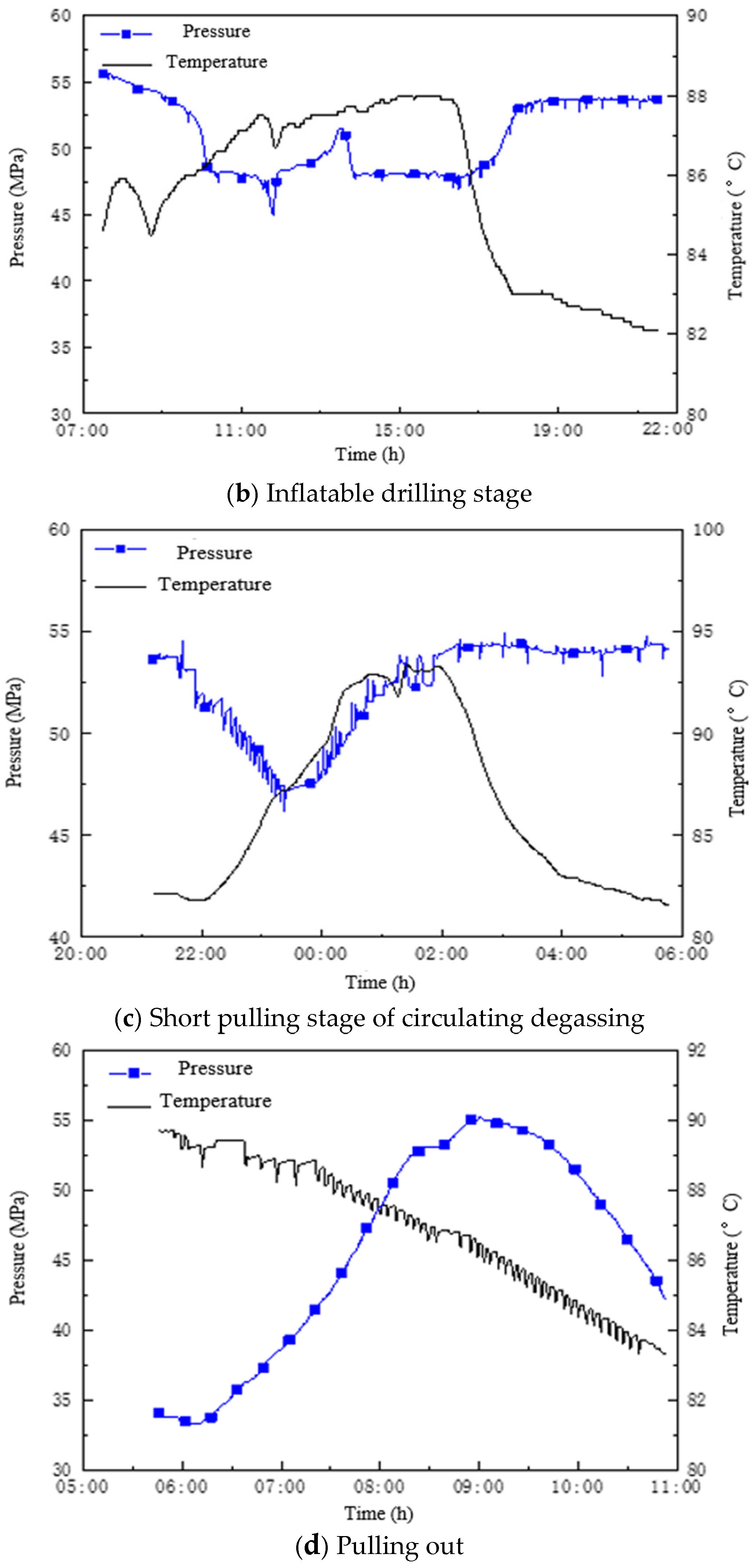
4. Field Test of Well Qing 2-76
5. Result and Discussion
Author Contributions
Funding
Data Availability Statement
Conflicts of Interest
References
- Guan, Z.; Han, Z.; Wang, Y. Development of a Kind of Device for Measuring the Force Acted on Drill String in Borehole. J. Univ. Pet. China 2002, 26, 30–35. [Google Scholar]
- Cui, X.; Guan, Z.; Han, Z.; Chen, Y.; Sun, C. Mechanical Structure Design and Manufacturing of Drill String Measurement Joints. J. Mach. Des. 2002, 30–32. [Google Scholar] [CrossRef]
- Wang, Y.; Guan, Z.; Li, Z.; Sun, C.; Han, Z. Development of an automatic measurement system for underground measurement joints. J. Pet. Univ. 2000, 24, 24–27. [Google Scholar]
- Wang, Y. A new intelligent bit design. Acta Pet. Sin. 2003, 24, 92–95. [Google Scholar]
- Wu, Z.; Yang, J.; Song, Y.; Yu, L. Measurement Instrument for Downhole Drilling Mechanical Parameters: China, 2003200105002.4. 28 June 2006. Available online: https://kns.cnki.net/kcms2/article/abstract?v=kxaUMs6x7-4I2jr5WTdXtkOSbVhUnTwoNPmGzaMv0X3fzdT73kQ5GKbPTJvGqefvCAfIAAx0ytYKCrCcDpkrfg%3d%3d&uniplatform=NZKPT (accessed on 5 May 2023).
- Wang, D.; Gao, D.; Gao, B.; Fu, Z.; Zhou, J. Research on the Function of the Mechanical Characteristics Measurement System for Drill String Near Drill Bit. Nat. Gas Ind. 2006, 26, 62–64. [Google Scholar]
- Yuan, X.; Liu, X.; Li, J.; Li, S. Preliminary Study on Improving the Drilling Speed of Deep and Large Wells by Drilling and Expanding Technology. West. Explor. Eng. 2010, 22, 78–81. [Google Scholar]
- Li, Y.; Wang, J.; Shan, Y.; Wang, C.; Hu, Y. Measurement and Analysis of Downhole Drill String Vibration Signal. Appl. Sci. 2021, 11, 11484. [Google Scholar] [CrossRef]
- Liu, M.B.; Liao, S.M.; Men, Y.Q.; Xing, H.; Liu, H.; Lian, Y. Field Monitoring of TBM Vibration During Excavating Changing Stratum: Patterns and Ground Identification. Rock Mech. Rock Eng. 2022, 55, 1481–1498. [Google Scholar] [CrossRef]
- Ma, H.; Yu, C.; Dong, L.; Fu, Y.; Shuai, C.; Sun, H.; Zhu, X. Review of intelligent well technology. Petroleum 2020, 6, 226–233. [Google Scholar]
- Pastorek, N.; Young, K.R.; Eustes, A. Downhole Sensors in Drilling Operations. In Proceedings of the 44th Workshop on Geothermal Reservoir Engineering Stanford University, Stanford, CA, USA, 11–13 February 2019; pp. 11–13. [Google Scholar]
- Lu, C.; Wu, M.; Chen, L.; Cao, W. An event-triggered approach to torsional vibration control of drill-string system using measurement-while-drilling data. Control Eng. Pract. 2021, 106, 104668. [Google Scholar] [CrossRef]
- Li, Y.W.; Ai, C.; Wang, Z.C.; Hu, C. Y; Hao M; Li S. Influencing factors of density window of safe drilling fluid in deep wells. Pet. Geol. Recovery Effic. 2013, 20, 107–110. [Google Scholar]
- Shen, J.W.; Wang, X.D.; Ding, J.X. Risk Recognition and Analysis of Drilling Accidents of Loss and Gush Stick in Deep Wells in Western Sichuan. Drill. Prod. Technol. 2017, 40, 10–12. [Google Scholar]
- Chen, S.Z. Research and Simulation of Dynamic Annular Pressure Control System; China University of Petroleum (East China): Dongying, China, 2011. [Google Scholar]
- He, Z.; Qiu, Y.; Liang, H.; Li, Y.; Yuan, X. Researchon remote intelligent control technology of throttling and back pressure in managed pressure drilling. Petroleum 2021, 7, 222–229. [Google Scholar]
- Sobie, C.; Capolungo, L.; McDowell, D.L.; Martinez, E. Thermal activation of dislocations in large scale obstacle bypass. J. Mech. Phys. Solids 2017, 105, 150–160. [Google Scholar] [CrossRef]
- Dunlap, P.H.; Steinetz, B.M.; De Mange, J.J. High Temperature Propulsion System Structural Seals for Future Space Launch Vehicles. In Proceedings of the 3rd Modeling and Simulation Joint Subcommittee Meeting, Colorado Springs, CO, USA, 1–5 December 2003; NASA/TM-2004-212907. [Google Scholar]
- Glass, D.; Dirling, R.; Croop, H.; Fry, T.; Frank, G. Materials Development for Hypersonic Flight Vehicles. In Proceedings of the 14th AIAA/AHI Space Planes and Hypersonic Systems and Technologies Conference, Canberra, Australia, 6–9 November 2006; AIAA-2006-8122. [Google Scholar]
- Zhu, W.; Shah, B.; Gorti, S.; Bhandari, M.; Adria, S.; Sabau, S.S. Effects of edge-seal design on the mechanical and thermal performance of vacuum-insulated glazing. Build. Environ. 2022, 224, 109572. [Google Scholar] [CrossRef]
- Proett, M.A.; Seifert, D.J.; Chin, W.C.; Lysen, S.; Sands, P. Formation testing in the dynamic drilling environment. In Proceedings of the PWLA 45th Annual Logging Symposium, Noordwijk, The Netherlands, 6–9 June 2004. [Google Scholar]
- Liu, Y.G.; Shao, T.B. Development and Application of Downhole Pressure and Temperature Testing Tools. Pet. Drill. Technol. 2004, 32, 27–31. [Google Scholar]
- Yang, H. Study on Determining Factors and Controlling Methods of Bottom Negative Pressure Difference in Underbalanced Drilling. Nat. Gas Ind. 2001, 21, 60–64. [Google Scholar]
- Liu, P.F.; Liu, L.Y.; Si, N.T.; Zhao, J.F.; Huang, Y.X.; Zuo, C.H. Application of Geo-Tap in Well E3S of Bozhong25-1 Oilfield. Pet. Drill. Technol. 2009, 37, 42–44. [Google Scholar]
- Wang, G.X.; Cao, H.P. Introduction and Application of Wireless Logging While Drilling System. Pet. Instrum. 2008, 22, 1–4. [Google Scholar]


| Number | Temperature/ ℃ | Pressure/ MPa | Pressure/ Psia | Temperature Frequency/ kHz | Pressure Frequency/ kHz | Temperature Value/ °C | Pressure Value/ Psia | Temperature Error/ °C | Pressure Error/ Psia |
|---|---|---|---|---|---|---|---|---|---|
| 1 | 22.8 | 0 | 14.6959 | 30.3177 | 27.5139 | 25.983 | 14.994 | 0.483 | 0.298 |
| 2 | 10 | 1465.0733 | 30.1345 | 31.0026 | 25.411 | 1464.958 | −0.089 | −0.115 | |
| 3 | 20 | 2915.4507 | 30.1218 | 34.4978 | 25.372 | 2914.807 | −0.128 | −0.644 | |
| 4 | 40 | 5816.2055 | 30.1154 | 41.5169 | 25.352 | 5814.760 | −0.148 | −1.445 | |
| 5 | 60 | 8716.9603 | 30.1148 | 48.5729 | 25.350 | 8714.907 | −0.150 | −2.053 | |
| 6 | 80 | 11,617.7151 | 30.1211 | 55.6640 | 25.370 | 11,615.322 | −0.130 | −2.393 | |
| 7 | 100 | 14,518.4699 | 30.1226 | 62.7881 | 25.374 | 14,515.556 | −0.126 | −2.914 | |
| 8 | 120 | 17,419.2247 | 30.1211 | 69.9436 | 25.370 | 17,415.717 | −0.130 | −3.508 | |
| 9 | 140 | 20,319.9795 | 30.1201 | 77.1222 | 25.367 | 20,313.363 | −0.133 | −6.617 | |
| 37 | 145 | 0 | 14.6959 | 74.0879 | 28.7700 | 145.153 | 16.429 | 0.153 | 1.733 |
| 38 | 10 | 1465.0733 | 74.1129 | 31.8531 | 145.210 | 1467.320 | 0.210 | 2.247 | |
| 39 | 20 | 2915.4507 | 74.1301 | 34.9426 | 145.249 | 2912.153 | 0.249 | −3.298 | |
| 40 | 40 | 5816.2055 | 74.1640 | 41.2021 | 145.326 | 5812.059 | 0.326 | −4.146 | |
| 41 | 60 | 8716.9603 | 74.1904 | 47.5468 | 145.386 | 8716.243 | 0.386 | −0.717 | |
| 42 | 80 | 11,617.7151 | 74.2244 | 53.9640 | 145.464 | 11,620.173 | 0.464 | 2.458 | |
| 43 | 100 | 14,518.4699 | 74.2496 | 60.4361 | 145.521 | 14,517.816 | 0.521 | −0.654 | |
| 44 | 120 | 17,419.2247 | 74.2748 | 66.9730 | 145.578 | 17,415.670 | 0.578 | −3.555 | |
| 45 | 140 | 20,319.9795 | 74.2925 | 73.5726 | 145.618 | 20,314.886 | 0.618 | −5.094 | |
| 46 | 175 | 0 | 14.6959 | 83.0425 | 29.5524 | 164.623 | 15.703 | −0.377 | 1.007 |
| 47 | 10 | 1465.0733 | 83.0763 | 32.5363 | 164.693 | 1466.826 | −0.307 | 1.753 | |
| 48 | 20 | 2915.4507 | 83.0947 | 35.5366 | 164.731 | 2915.696 | −0.269 | 0.245 | |
| 49 | 40 | 5816.2055 | 83.1267 | 41.6120 | 164.797 | 5817.589 | −0.203 | 1.383 | |
| 50 | 60 | 8716.9603 | 83.1636 | 47.7713 | 164.874 | 8718.270 | −0.126 | 1.310 | |
| 51 | 80 | 11,617.7151 | 83.1869 | 54.0092 | 164.922 | 11,617.294 | −0.078 | −0.421 | |
| 52 | 100 | 14,518.4699 | 83.2093 | 60.3259 | 164.968 | 14,516.555 | −0.032 | −1.915 | |
| 53 | 120 | 17,419.2247 | 83.2330 | 66.7156 | 165.017 | 17,415.848 | 0.017 | −3.377 | |
| 54 | 140 | 20,319.9795 | 83.2527 | 73.1731 | 165.058 | 20,315.555 | 0.058 | −4.425 |
| Density | 1.15 g/cm3 | Viscosity | 97 s |
|---|---|---|---|
| Sand-carrying capacity | 0.3% | Medium pressure dehydration | 3.8 mL |
| Shearing force | 6/17 | Mud cake thickness | 0.5 mm |
| PH | 9 | drilling footage | 15 m/h |
Disclaimer/Publisher’s Note: The statements, opinions and data contained in all publications are solely those of the individual author(s) and contributor(s) and not of MDPI and/or the editor(s). MDPI and/or the editor(s) disclaim responsibility for any injury to people or property resulting from any ideas, methods, instructions or products referred to in the content. |
© 2023 by the authors. Licensee MDPI, Basel, Switzerland. This article is an open access article distributed under the terms and conditions of the Creative Commons Attribution (CC BY) license (https://creativecommons.org/licenses/by/4.0/).
Share and Cite
Lu, M.; Liao, H.; Wang, H.; He, Y.; Liu, J.; Wang, Y.; Niu, W. Research and Test on the Device of Downhole Near-Bit Temperature and Pressure Measurement While Drilling. Processes 2023, 11, 2238. https://doi.org/10.3390/pr11082238
Lu M, Liao H, Wang H, He Y, Liu J, Wang Y, Niu W. Research and Test on the Device of Downhole Near-Bit Temperature and Pressure Measurement While Drilling. Processes. 2023; 11(8):2238. https://doi.org/10.3390/pr11082238
Chicago/Turabian StyleLu, Ming, Hualin Liao, Huajian Wang, Yuhang He, Jiansheng Liu, Yifan Wang, and Wenlong Niu. 2023. "Research and Test on the Device of Downhole Near-Bit Temperature and Pressure Measurement While Drilling" Processes 11, no. 8: 2238. https://doi.org/10.3390/pr11082238