A Mathematical Model for Force Prediction in Single Point Incremental Sheet Forming with Validation by Experiments and Simulation

Abstract

Incremental sheet forming (ISF) is an emerging technology that has shown great potential in forming customized three-dimensional (3D) parts without the use of product-specific dies. The forming force is reduced in ISF due to the localized nature of deformation and successive forming. Forming force plays an important role in modeling the process accurately, so it needs to be evaluated accurately. Some attempts have been made earlier to calculate the forming force; however, they are mostly limited to empirical formulae for evaluating the average forming force and its different components. The current work presents a mathematical model for force prediction during ISF in a 3D polar coordinate system. The model can be used to predict forces for axis-symmetric cones of different wall angles and also for incremental hole flanging. Axial force component, resultant force in the r-θ plane, and total force have been calculated using the developed mathematical model appearing at different forming depths. The cone with the same geometrical parameters and experimental conditions was modeled and simulated on ABAQUS, and finally, experiments were carried out using a six-axis industrial robot. The mathematical model can be used to calculate forces for any wall angle, but for comparison purposes, a 45° wall angle cone has been used for analytical, numerical, and experimental validation. The total force calculated from the mathematical model had a very high level of accuracy with the force measured experimentally, and the maximum error was 4.25%. The result obtained from the FEA model also had a good level of accuracy for calculating total force, and the maximum error was 4.89%.

1. Introduction

Incremental Sheet Forming (ISF) is a flexible manufacturing process because complex three-dimensional (3D) parts can be fabricated by using only specific tool path programming on the existing setup without the use of dedicated dies. It is widely used for small batches and customized production. Patented in 1967, the process has attracted the eyes of aerospace, automotive [1], and biomedical sectors [2] for manufacturing complex sheet metal components. The process was used by Iseki et al. [3] for small batch production of non-symmetrical shallow shells using path-controlled spherical rollers. Various shapes were produced using the process of ISF, and a bulging test was used to predict the forming limit of ISF. In ISF, necking is either suppressed or delayed, due to which higher strains can be induced than in conventional stamping, deep drawing, and stretching processes [4].

Since the establishment of the process, there have been numerous attempts to establish the mechanism of ISF. Several FEA and theoretical analyses have been done to understand the underlying mechanism of the process. Initially, it was understood that the underlying mechanism behind the process is near biaxial stretching, as confirmed by Shim and Park [5] by FEA modeling. They concluded that Near Biaxial Stretching occurs in the closed loop, and near plane strain occurs along the straight line. They further concluded that the Forming Limit Curve (FLC), which is a plot of major strain vs. minor strain for ISF, is a straight line with a negative slope in the positive direction of minor strain and recommended the straight groove test as a standard test for plotting FLC for ISF [5]. Kim and Park predicted the same results by performing a series of experiments to produce various shapes [6].

Sheet thickness in the ISF process can be approximated by the famous sine law $t=t_0\sin \theta$, where $\theta$ is the wall angle in the formed conical part. Since the thickness in the case of shear spinning is also given by the same sine law, the underlying deformation mechanism, as established by Avitzur and Yang [7] and demonstrated mathematically by Kim et al. [8], was initially considered to be pure shear through the thickness of the sheet and plane strain in the plane parallel to the undeformed sheet. Jackson et al. [9] found the presence of through-thickness shear along tool movement by measuring relative displacement in the sandwich panel. They took two pieces of 3 mm thick copper sheet, engraved their cross-section with square mesh, and brazed them. This method was adopted and suggested by Kalpakcioglu [10]. After deformation, they measured the mesh configuration and found the presence of through-thickness shear in the tool direction [11]. The presence of out-of-plane through-thickness stresses can lead to improved formability in the case of ISF, as suggested by Ma and Wang [12]. They further suggested that the conventional M-K model, which includes in-plane stresses only, needs to be extended and should also consider the through-thickness shear stresses. Allwood and Shoulder [13] proposed a generalized forming limit diagram (GFLD) that considered the out-of-plane stresses. It is evident that the stress state in ISF is complex, which was studied by Emmens and Boogard [14], and they presented an overview of the mechanisms responsible for higher strain in the single-point incremental forming (SPIF) process. They suggested that there are various factors responsible for higher strain in the ISF process. The nature of the complex stress state also plays a vital role in the higher strains in ISF [15]. Eyckens et al. [16] demonstrated, through finite element modeling, the presence of shear in the direction of tool movement but only a little shear in the perpendicular direction [8]. In addition to shear in the tool direction, Bending Under Tension (BUT) also plays a role in the enhancement of formability. Sawada et al. [17] performed a numerical study of stretch forming and ISF and found that bending and unbending happen along the meridional line, and shear happens along the circumferential direction. They also concluded that necking is induced on the part of the sheet which is in contact with the punch and stops after the punch surpasses the necking point. Recently, Li et al. [18] used the FE model to affirm that the deformation mechanism in ISF is a combination of bending, stretching, and shear.

Even after so many attempts, the underlying deformation mechanism of the process is still not clear due to the evolution of the complex stress state during the process. However, it can be said with affirmation that the stress state appearing during ISF consists of shear, normal, and bending stresses. Understanding of deformation mechanism is pivotal in developing an analytical model for force prediction in the process. Therefore, for developing such a model, all the stress components must be taken into consideration.

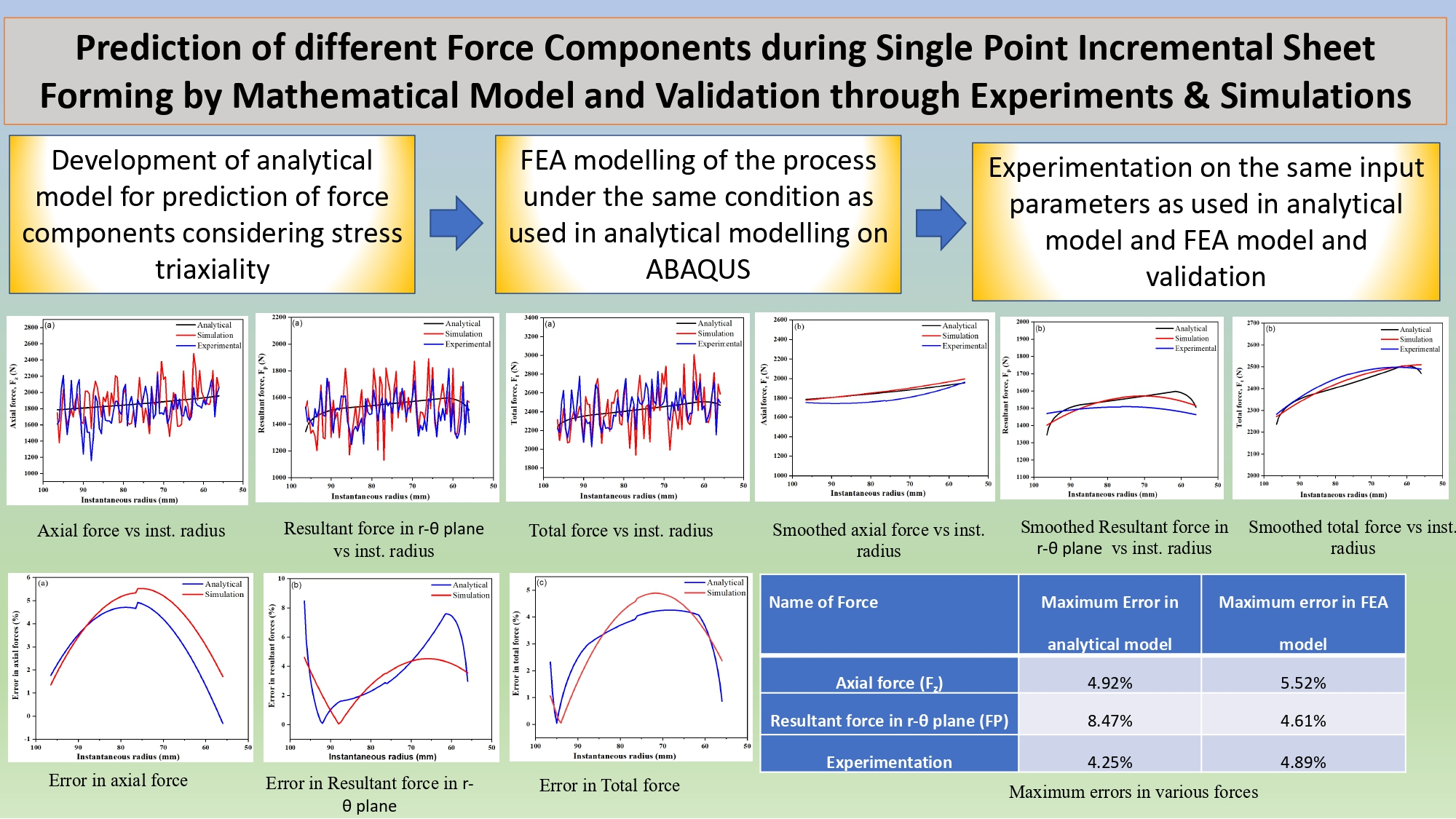
For in situ measurement of forces appearing during the ISF process, a dynamometer is fixed on the tool, and it measures the forces appearing during forming. The forces acting in ISF are (a) the axial force (F_z), acting in the direction along the tool axis, (b) force in the radial direction (F_r), and (c) force along the tangential direction (F_θ). The vector diagram of forces appearing during the process is given in Figure 1. Recently, Kumar et al. [19] presented a comprehensive review of the state of the arts of forming force and their effects on various forming outputs.

Duflou et al. [20] presented a model based on regression equations for force prediction during cone forming by SPIF as a function of step size, wall angle, tool diameter, and sheet thickness. Duflou et al. [21] performed a large set of experiments to form empirical relations for the calculation of force components for five different materials: AA3033, AA5754, DC01, AISI 304, and spring steel 65Cr₂. Saidi et al. [22] conducted a set of experiments on sheets of AA1050 and 304 steel and validated their results, as predicted by Jeswiet et al. [23] and Aerens et al. [21]. Xiao et al. [24] measured forming forces by an in situ force monitoring system and studied the effect of forming temperature on the forming of an AA7075-T6 sheet. They found that the peak force was reduced to 1300 N from 1900 N when forming temperature was increased from 140 to 200 °C.

In addition to various experimental measuring methodologies, numerous attempts have been made to develop analytical and FEA models, considering various deformation mechanisms based on available literature for the calculation of forces and other parameters like strain, thickness, etc., during the process.

Flores et al. [25] used the FEA simulation of SPIF and studied the effects of constitutive laws on force prediction. They concluded that the selection of constitutive laws plays a vital role in force prediction, as the results were different for elastoplastic laws with isotropic and kinematic hardening. Henrard et al. [26] used FEA simulation to predict the forces for 20° and 60° cones using the Lagamine model, first-order brick element model for various simulation parameters, and inverse method for material data fit. They also conducted experiments for the validation of results obtained from FE modeling. Honarpisheh et al. [27] performed FEM analysis on ABAQUS to predict forces appearing during forming of Al/Cu bimetals and studied the effects of various parameters in ISF.

Iseki [28] used the equilibrium of the shell element to model bulge height, strain, and load during the process. He also used FEA analysis for validation of the results of the theoretical model. Silva et al. [29] proposed membrane analysis to consider the friction between the tool and sheet for analysis of the small plastic zone created during forming of symmetrical axis shapes in SPIF. They proposed that friction stress at the contact between tool and sheet can be assumed to be made of a couple of in-plane components, viz. meridional component (${\mu }_{\Phi }{\sigma }_t$) and circumferential component (${\mu }_{\theta }{\sigma }_t$). They considered the thickness, meridional, and circumferential direction as principal directions and gave the following equations for the corresponding stresses:

$${\sigma }_t=-\frac{{\sigma }_{Y}t}{{(r}_{tool}+t)}$$

(1)

$${\sigma }_{\Phi }=\frac{{\sigma }_Y{r}_{tool}}{{(r}_{tool}+t)}$$

(2)

$${\sigma }_{\theta }=\frac{{\sigma }_Y{(r}_{tool}-t)}{2{(r}_{tool}+t)}$$

(3)

Further, Chang et al. [30] used membrane analysis for the analytical modeling of the single-pass and multi-pass incremental sheet forming process (MPISF) and incremental hole flanging process (IHF). Bansal et al. [31] used the above equations for force calculation for single-stage and multi-stage ISF, modeling the contact area and validating with experiments and the formula given by Duflou et al. [20]. Similarly, Fang et al. [32] did analytical modeling of the process and validated it with numerical modeling, and also studied the fracture behavior of the sheet in ISF. Liu et al. [33] modeled the process in the 3D polar coordinate system and validated it experimentally. They further extended their work [34] and gave a comprehensive analytical model for the prediction of forming forces in three directions and studied the effect of step depth, tool diameter, and sheet thickness on forming forces occurring in ISF.

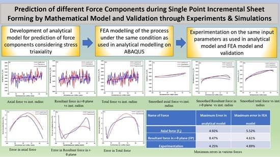
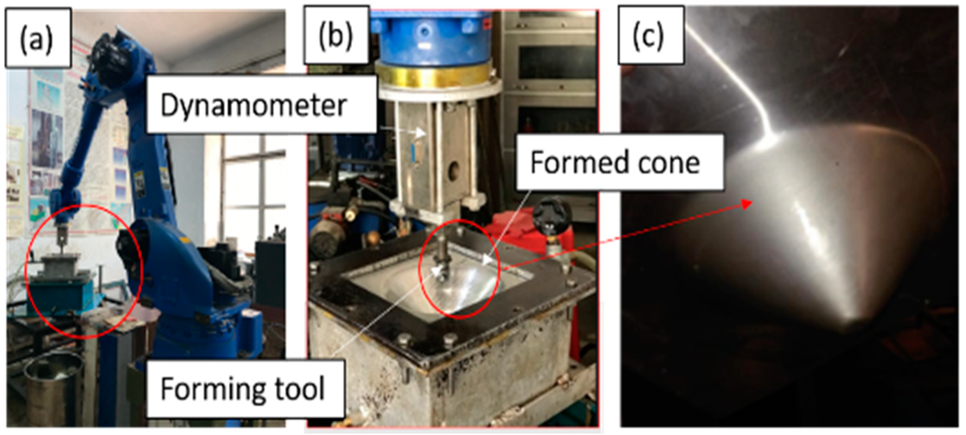
It can be concluded from the literature survey that although attempts have been made to develop a mathematical model of ISF, a comprehensive model for force prediction has not been established yet. Further, most of the models are empirical in nature, and they are used to calculate average forces during the process. Some other models consider only plane stresses in thickness, meridional, and circumferential direction and do not consider shear stresses. Very few works have been done considering all the six stress components to finally arrive at forces. In this current work, a simple mathematical model for the ISF process has been developed in a cylindrical coordinate system considering all the stress components. All force components have been calculated at different forming depths where the tool moves in different radii. The obtained results have been compared with the FEA model developed using the ABAQUS platform. Finally, experiments have been performed on aluminum alloy 6061 on a six-axis industrial robotic arm with the same experimental conditions as used for the analytical and FEA model. Different force components were measured using a dynamometer mounted on the robotic arm. The obtained results for various force components and total force have been compared.

2. Mathematical Model Development

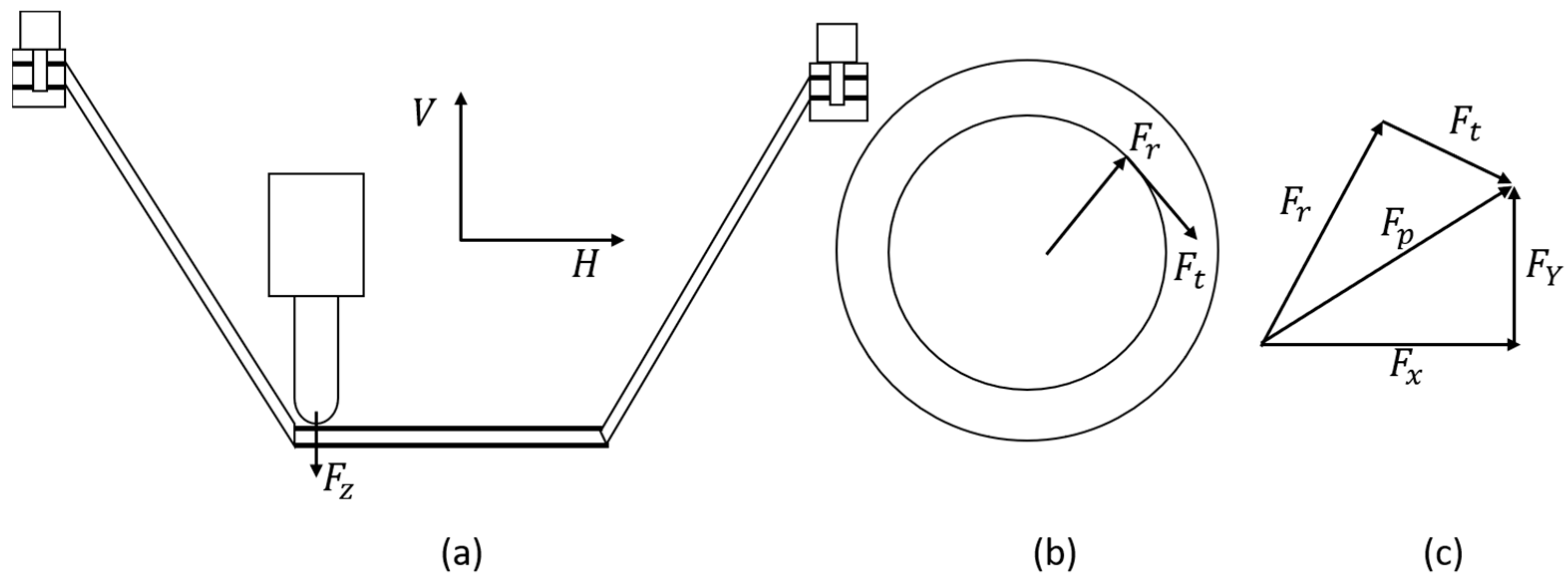
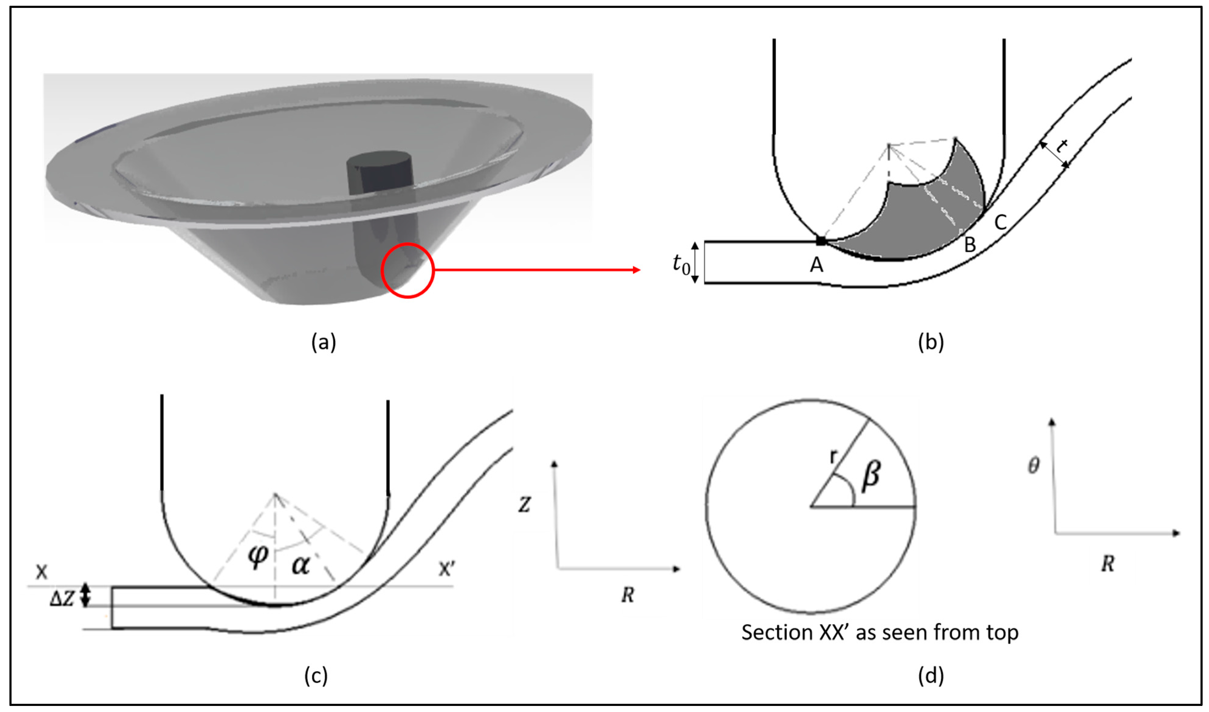
For solving the mathematical equations, the cylindrical 3D coordinate has been chosen as tool motion to give a conical shape that can be easily replicated in this coordinate system. The center of the undeformed sheet has been chosen as the origin of the global coordinate system. The element has been taken in a local 3D polar co-ordinate system which is at a forming depth h and of length rdθ in the radial direction at an angle θ in the circumferential direction on the surface of the sheet in contact with the tool in the local polar coordinate system, as shown in Figure 2a,b. It is worth noting that the three directions—radial (r-direction), circumferential (θ-direction), and axial (z-direction)—may not necessarily be the principal directions. Hence all the six-stress component has been considered.

A few assumptions listed below have been made to develop the model:

• All body forces have been neglected during the analysis;
• ${\tau }_{\theta z}$ has been neglected throughout the analysis;
• Normal stress in radial and z-directions are distributed in the same ratio as that of increments provided in this direction for forming a fixed wall angle cone. $\frac{\partial r}{\partial z}=\tan \alpha$, $\frac{{\sigma }_{rr}}{{\sigma }_{zz}}=\tan \alpha$, where $\alpha$ is the wall angle of the formed cone. The wall angle and step depths can be understood in Figure 3a;
• For a given radius in which the tool is moving, ${\tau }_{r\theta }$ varies only along $\theta$ direction. If the considered element is under static equilibrium, the equilibrium equations in the differential form can be written directly [35]. The free-body diagram of the considered element is given in Figure 3b. Neglecting body forces, the equilibrium equations in the respective directions are:

In radial direction

$$\frac{\partial {\sigma }_{rr}}{\partial r} + \frac{1}{r}\frac{\partial {\tau }_{r\theta }}{\partial \theta } + \frac{{\sigma }_{rr}-{\sigma }_{zz}}{r} + \frac{\partial {\tau }_{rz}}{\partial z}=0$$

(4)

In circumferential direction

$$\frac{\partial {\tau }_{r\theta }}{\partial r}+\frac{1}{r}\frac{\partial {\sigma }_{\theta \theta }}{{\partial }_{\theta }}+\frac{2}{r}{\tau }_{r\theta }=0$$

(5)

In z direction

$$\frac{\partial {\tau }_{rz}}{\partial r}+\frac{{\tau }_{rz}}{r}+\frac{1}{r}\frac{\partial {\tau }_{\theta z}}{\partial \theta }+\frac{\partial {\sigma }_{zz}}{\partial z}=0$$

(6)

The major shear component has been assumed to act only along the radial direction only. Hence ${\tau }_{\theta z}$ has been neglected throughout the model. Further, from membrane analysis, it can be said that

$${\tau }_{rz}=f{\sigma }_{rr},$$

(7)

Using the membrane analysis (4) and Equation (1) becomes

$$\frac{\partial {\sigma }_{rr}}{{\partial }_r} + \frac{1}{r}\frac{\partial {\tau }_{r\theta }}{\partial \theta } + \frac{{\sigma }_{rr}-{\sigma }_{\theta \theta }}{r} + f\frac{\partial {\sigma }_{rr}}{\partial z} = 0$$

(8)

Membrane analysis (4) and the assumption 2, Equation (3) becomes

$$f\frac{\partial {\tau }_{rr}}{{\partial }_r}+f\frac{{\partial }_{rr}}{r}+\frac{\partial {\sigma }_{zz}}{\partial z}=0$$

(9)

For any incremental sheet forming, the fabrication of 3D shapes is done by making the tool move over the sheet and providing increments to the tool so that it can perform fabrication in different passes. For fabricating a conical wall, the increments are provided in vertical and horizontal directions. In the current work, the increments are provided in radial and the vertically downward direction. These increments are generally small in comparison to r, and if the given assumption holds, then it can be assumed that, on neglecting spring back

$△z=△r \tan \alpha$, where $△z$ is the increment in the vertical direction and $△r$ is the increment in radial direction. If these are small, then

$$\partial r \tan \alpha = \partial z$$

(10)

Using assumption 3, it can be directly said that normal stress in radial and z-directions are distributed in the same ratio as that of increments.

$${\sigma }_{rr}\tan \alpha = {\sigma }_{zz}$$

(11)

Taking differentials on both sides, it can be said that

$$\partial {\sigma }_{rr}\tan \theta = \partial {\sigma }_{zz}$$

(12)

From (7) and (8), it can be said that

$$\frac{\partial {\sigma }_{rr}}{\partial r} = \frac{\partial {\sigma }_{zz}}{\partial z}$$

(13)

Using Equation (9), Equation (6) further converges to

$$f\frac{\partial {\sigma }_{rr}}{\partial r}+f\frac{{\sigma }_{rr}}{r}+\frac{\partial {\sigma }_{rr}}{\partial r}=0$$

(14)

$$\frac{\partial {\sigma }_{rr}}{\partial r}(1+f)=-f\frac{{\sigma }_{rr}}{r}$$

(15)

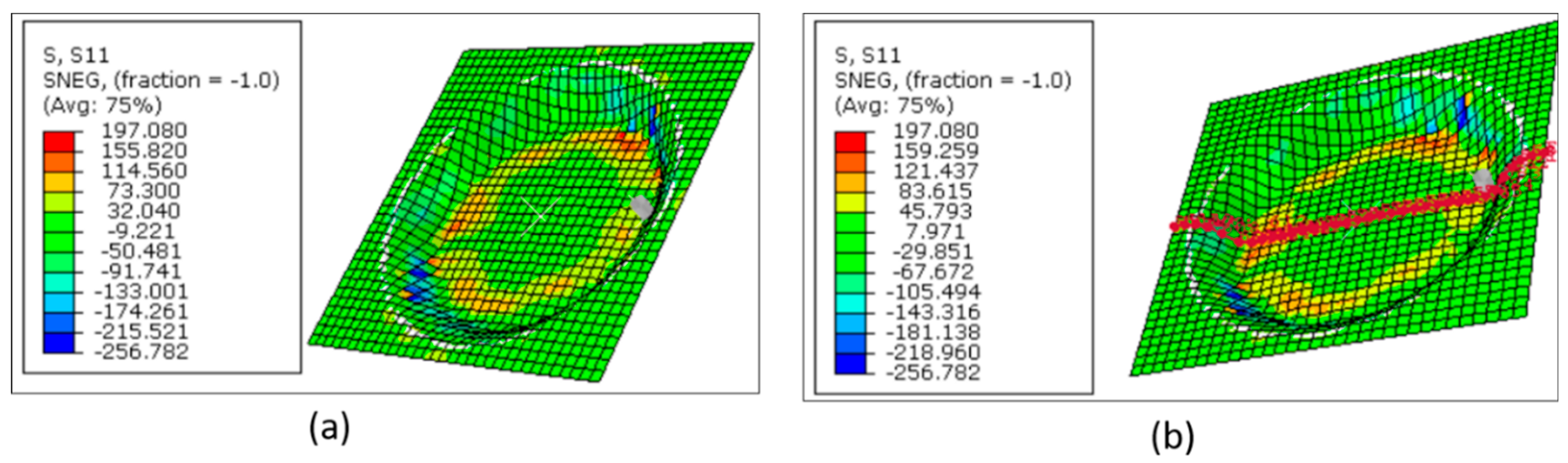
Taking integrals on both sides of the above relation

$$\int \frac{\partial {\sigma }_{rr}}{{\sigma }_{rr}}=\int \frac{\partial r}{r}\left\{\frac{-f}{1+f}\right\}$$

$${ln\sigma }_{rr}=ln{r}^{\frac{-f}{1+f}}+ln C$$

(16)

$${\sigma }_{rr}=\frac{c}{r^{\frac{f}{1+f}}}$$

(17)

From the above analysis, it is evident that for one complete cycle, the stress in the radial direction is constant. This analysis was performed on ABAQUS with the same parameters as used for the analytical model, and considering the element when the instantaneous radius of the undeformed part is 82.5 mm, the RMS value of the S₁₁ was found to be approximately equal to 140 MPa as shown in Figure 3.

For $f=\frac{1}{\sqrt{3}}$, C = 292.5

$${\sigma }_{rr}=\frac{292.5}{r^{0.1667}}$$

(18)

Since ${\sigma }_{rr}$ depends on instantaneous circle radius only, hence

$$\frac{\partial {\sigma }_{rr}}{\partial z}=0$$

(19)

From the equilibrium equation in the r-direction, we have

$$\frac{\partial {\sigma }_{rr}}{\partial r}+\frac{1}{r}\frac{\partial {\tau }_{r\theta }}{\partial z}+\frac{{\sigma }_{rr-}{\sigma }_{\theta \theta }}{r}+\frac{\partial {\sigma }_{rr}}{\partial z}=0$$

(20)

Using Equations (18) and (20)

$$\frac{\partial }{\partial r}\left\{\frac{C}{r^{\frac{f}{1+f}}}\right\}+\frac{1}{r}\frac{\partial {\tau }_{r\theta }}{{\partial }_{\theta }}+\frac{C}{r(r^{\frac{f}{1+f}})}=\frac{{\sigma }_{\theta \theta }}{r}$$

(21)

We can directly say this using Equation (17)

$${\sigma }_{rr}\left\{1-\frac{f}{f+1}\right\}+\frac{{\partial \tau }_{r\theta }}{{\partial }_{\theta }}={\sigma }_{\theta \theta }$$

(22)

$$\frac{\partial {\tau }_{r\theta }}{\partial \theta } = {\sigma }_{\theta \theta } - \frac{{\sigma }_{rr}}{(1+f)}$$

(23)

In the circumferential direction, using assumption 4, hence the equation in the circumferential direction converges to

$$\frac{1}{r}\frac{{\partial \sigma }_{\theta \theta }}{{\partial }_{\theta }}+\frac{2}{r}{\tau }_{r\theta }=0$$

(24)

$$\frac{{\partial \sigma }_{\theta \theta }}{{\partial }_{\theta }}=-2{\tau }_{r\theta }$$

(25)

From Equations (23) and (25), we have

$$\frac{{\partial \tau }_{r\theta }}{{\partial \sigma }_{\theta \theta }}=\left(\frac{{\sigma }_{\theta \theta }-\frac{{\sigma }_{rr}}{\left(1+f\right)}}{2{\tau }_{r\theta }}\right)$$

$$2\int {\tau }_{r\theta }{\partial \tau }_{r\theta }=-\int {\sigma }_{\theta \theta }{\partial \sigma }_{\theta \theta }+\frac{{\sigma }_{rr}}{(1+f)}\int {\partial \sigma }_{\theta \theta }$$

(26)

$${\left({\tau }_{r\theta }\right)}^2=\frac{{\sigma }_{rr}{\sigma }_{\theta \theta }}{(1+f)}-\frac{{\left({\sigma }_{\theta \theta }\right)}^2}{2}+k^{\prime }$$

(27)

$$\mathrm{If} {\sigma }_{\theta \theta }=0, {\tau }_{r\theta }=0, k^{\prime }=0$$

$${\left({\tau }_{r\theta }\right)}^2={\sigma }_{\theta \theta }\left\{\frac{{\sigma }_{rr}}{\left(1+f\right)}-\frac{{\sigma }_{\theta \theta }}{2}\right\}$$

(28)

From Von-Mises criteria, we have

$${({\sigma }_{rr}-{\sigma }_{\theta \theta })}^2+{({\sigma }_{rr}-{\sigma }_{zz})}^2+{({\sigma }_{\theta \theta }-{\sigma }_{zz})}^2+6\left[{{\tau }_{r\theta }}^2+{{\tau }_{rz}}^2+{{\tau }_{\theta z}}^2\right]={\stackrel{-}{\sigma }}^2$$

(29)

The model is valid for all wall angles; however, for validation purposes, a 45° wall angle has been chosen because of its simplicity.

$$\theta ={45}^{°},{\sigma }_{rr}={\sigma }_{zz},{\tau }_{\theta z}=0$$

$${2({\sigma }_{rr}-{\sigma }_{\theta \theta })}^2+6\left[{{\tau }_{r\theta }}^2+f^2{{\sigma }_{rr}}^2\right]={\stackrel{-}{\sigma }}^2$$

(30)

$${{\sigma }_{rr}}^2\left(2+6f^2\right)-{{\sigma }_{\theta \theta }}^2+{\sigma }_{\theta \theta }{\sigma }_{rr}\left(\frac{2-4f}{1+f}\right)={\stackrel{-}{\sigma }}^2$$

(31)

If we consider the strain to be acting from bending and stretching only [34], we have from volume conservation

$${\epsilon }_{\theta }+{\epsilon }_r+{\epsilon }_f=0$$

(32)

Total bending strain can be given by,$ln\left(\frac{r_{tool}}{R_m}\right)$

Whereas total tensile strain can be given as, ${\epsilon }_{stretching}=ln\left(\frac{t_0}{t}\right)$

Total strain can be given by

$$\epsilon =ln\left(\frac{r_{tool}}{R_m}\frac{t_0}{t}\right)$$

(33)

$${\left({\sigma }_{rr}\right)}^2\left(2+6f^2\right)-{{\sigma }_{\theta \theta }}^2+{\sigma }_{\theta \theta }{\sigma }_{rr}\left(\frac{2-4f}{1+f}\right)={\stackrel{-}{\sigma }}^2$$

(34)

Taking the simple power law for annealed sheet, we have $\stackrel{-}{\sigma }=$ ${K\epsilon }^n$. From tensile test we have K = 205 MPa, and n = 0.2

$${\left({\sigma }_{rr}\right)}^2\left(2+6f^2\right)-{{\sigma }_{\theta \theta }}^2+{\sigma }_{\theta \theta }{\sigma }_{rr}\left(\frac{2-4f}{1+f}\right)=K^2\left(\frac{4}{3}\right){\left[ln\frac{r_{tool}{t}_0}{R_{m}t}\right]}^{2n}$$

(35)

From the analytical model developed, it can be said that the stress state appearing during the process is complex, but a few simple conclusions can be summarized:

(a)

The largest stress component is normal stress on the theta plane along the tool movement direction. Appreciable shear stress appears in the direction perpendicular to the tool motion along the radial and z planes;

(b)

From the Equation (28), it is clear that

$$\frac{{\sigma }_{rr}}{\left(1+f\right)}>\frac{{\sigma }_{\theta \theta }}{2}$$

(36)

3. Contact Area Model

For contact area estimation, the approach of Bansal et al. [31] has been implemented. The contact area has been divided into two parts. The area directly below the tool in the region below the top of the undeformed sheet and the area above the undeformed sheet, as shown in Figure 4a,b. The area above the undeformed sheet leaves contact with the sheet tangentially in the circumferential direction. Let section XX′ be cut, and the top sectioned view is shown in Figure 4c.

From Figure 5b, it can be directly said that

$$\cos \phi =\frac{R-∆Z}{R}$$

(37)

The area of portion AB can be directly estimated by considering the concept of solid angle. The area can be given by

$$A_{AB}=2\pi R∆Z$$

(38)

The area of the portion above the top of the undeformed surface can be given by integrating the perimeters of the strips of width $d\theta$ taken at an angle $\theta$ the length of which will be rβ where r = R sin $\theta$

$$A_{AB}=\int PRd\theta =\int R^2\beta \sin \theta d\theta$$

(39)

As $\theta \mathrm{goes} \mathrm{from} \phi \mathrm{to} \alpha ,\beta \mathrm{goes} \mathrm{from}\raisebox{1ex}{$\pi $}\!\left/ \!\raisebox{-1ex}{$2$}\right.$ to 0.

Taking the variation of β to be linear with $\theta$, we have $(\beta -0)=\frac{-\pi }{2(\alpha -\phi )}(\theta -\alpha )$

$$\beta =\frac{\pi }{2\left(\phi -\alpha \right)}\left(\theta -\alpha \right)$$

(40)

From (39) and (40), we obtain

$$A_2=\frac{R^2\pi }{2\left(\phi -\alpha \right)}{\int }_{\phi }^{\alpha }(\theta -\alpha )\sin \theta d\theta$$

(41)

$$A_2=\frac{\pi R^2}{2\left(\phi -\alpha \right)}\left[\sin \alpha +\left(\phi -\alpha \right)\cos \phi -\sin \phi \right]$$

(42)

The total area of contact can be given by

$$A_T=\frac{\pi R^2}{2\left(\phi -\alpha \right)}\left[\sin \alpha +\left(\phi -\alpha \right)\cos \phi -\sin \phi \right]+2\pi R∆Z$$

(43)

$$A_T=\frac{\pi R}{2}\left(R+3∆z\right)-\frac{\pi R^2}{2\left(\alpha -\phi \right)}\left[\sin \alpha -\sin \phi \right]$$

(44)

Putting R = 5 mm, $∆z=0.5$, $\alpha =\frac{\mathsf{\pi }}{4}$ and $\phi =\frac{5\mathsf{\pi }}{36}, A_T=19.05$.

Considering the whole contact area as a rectangle of $\left(l\times b\right) \mathrm{area}$.

$l=R\left(\phi +\alpha \right)$ = 6.10 $\mathrm{mm}$ and b = 3.11 mm, the length of the portion above the top of the undeformed sheet is $l_{CD}=R\left(\alpha -\phi \right)=1.75\mathrm{mm}$.

$$\mathrm{Total} \mathrm{projected} \mathrm{area} \mathrm{in} Z - \mathrm{plane} = \left(R\sin \alpha \right)b \sin \alpha =7.775 {\mathrm{mm}}^2$$

(45)

$${\mathrm{Total} \mathrm{projected} \mathrm{area} \mathrm{in} r-\mathrm{plane}=A}_r=\left(\Delta Z+R\left(\cos \phi -\cos \alpha \right)\right)b\sin \alpha =3.28 {\mathrm{mm}}^2$$

(46)

$${\mathrm{Total} \mathrm{projected} \mathrm{area} \mathrm{in} \theta -\mathrm{plane}=A}_{\theta }=tl=4.52{\mathrm{mm}}^2$$

(47)

Different forces acting on the sheet in the contact region can be represented by the force diagram as given in Figure 1.

$$F_r={\sigma }_{rr}\times A_r+z_{r\theta }{A}_{\theta }+z_{rz}{A}_z$$

(48)

$$F_z={\sigma }_{zz}{A}_z+z_{rz}{A}_r$$

(49)

$$F_{\theta }={\sigma }_{\theta \theta }{A}_{\theta }+z_{r\theta }{A}_r$$

(50)

Once the relations for various force components were established, the calculation for forces using different developed equations was done on MATLAB for different instantaneous radii. The whole process was modeled on ABAQUS, and average forming forces were evaluated from the FEA model for the same instantaneous radii. The values obtained from the analytical model were compared with FEA and experimental results, as discussed in subsequent sections.

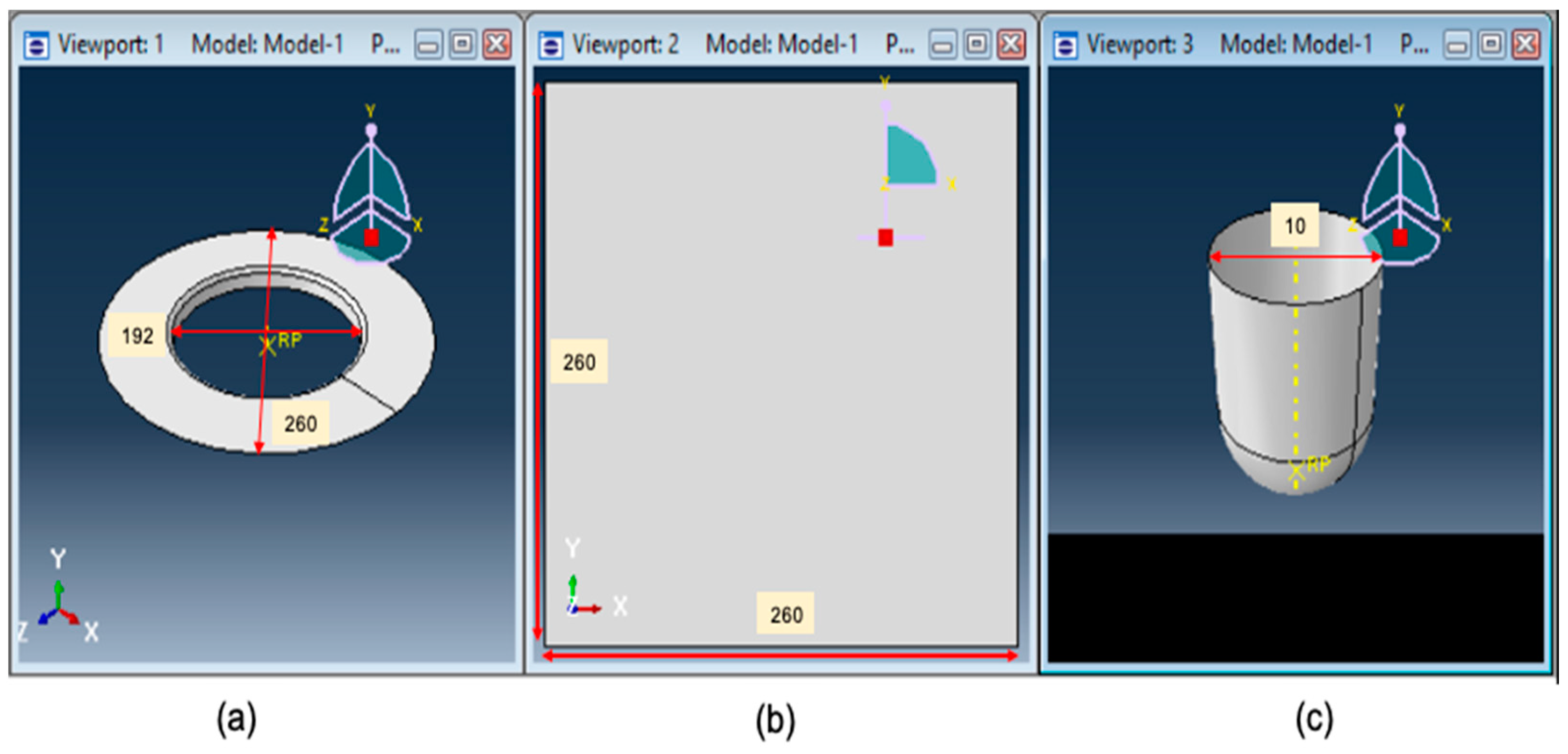
4. Simulation Study

The simulation analysis on the formed cone was carried out on ABAQUS. The finite element model was made on the software, which consisted of a rigid tool with a tool diameter of 10 mm, a deformable aluminum alloy 6061 sheet of thickness 1.05 mm, and a flange to hold the sheet. The geometry of the model used for simulation is given in Figure 5.

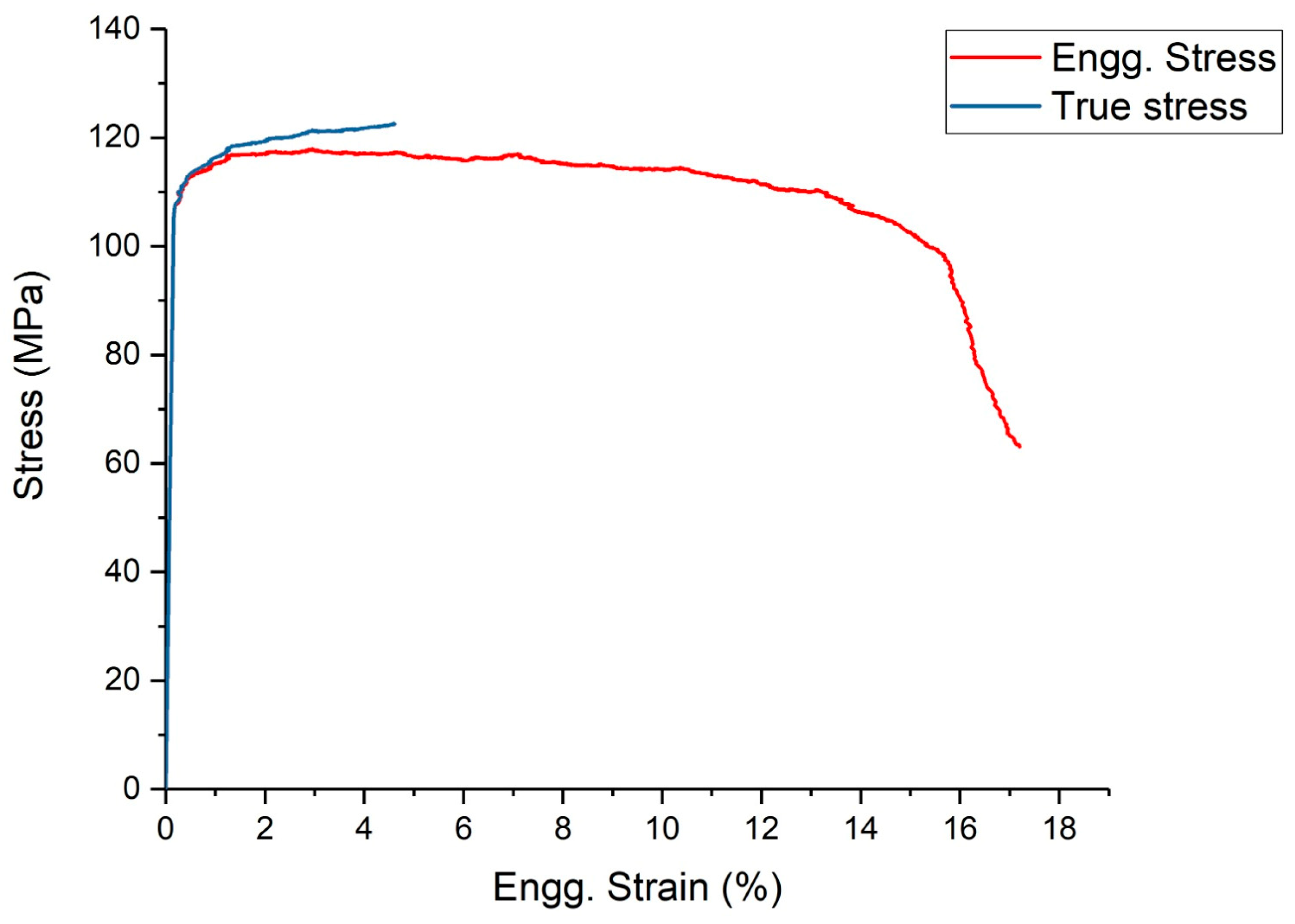
The properties of the material used in the simulation were obtained from the uniaxial tensile test and are given in

Table 1. Details of parameters used for simulation on ABAQUS.

Properties Used in Simulation	Corresponding Values
0.2% offset yield strength (MPa)	111
UTS(MPa)	119
Total Elongation	16.1%
Strength coefficient	205 MPa
Strain hardening exponent	0.2
Coefficient of Friction between tool and blank	0.2
Hardening model used	Isotropic
Mesh Size	6.96 mm
Mesh Type	Square
No. of elements taken	101 × 101
Simulation Run time	28 h

.

For simulation, a true stress-true strain curve up to maximum load was obtained from the tensile test. Since a large strain is obtained in ISF for post-necking values of true stress and true strain, the following method was adopted. The log-log plot of true stress and the true strain was made till necking. Thereafter, a linear relation was assumed between the logarithm of true stress and the logarithm of true strain from necking to fracture. The strain hardening exponent in this region can be evaluated by finding the slope of this linear portion of the plot from necking to fracture. In this way, the true stress-true strain data was obtained and fed in ABAQUS till fracture. The engineering and true stress-strain curve obtained after tensile testing is given in Figure 6.

The isotropic hardening model was used for analysis as the sheet was annealed. Square meshing was done on the plate and tool with an average mesh size of 6.96 mm.

Loading and Boundary condition:

Penalty contact between the tool and sheet was taken with the coefficient of friction between the tool and the sheet to be 0.2, which was obtained from the wear test. The boundary of the sheet was encastred, and the blank was made rigid and encastred. The tip of the tool was chosen as a reference point and was given corresponding motions as per the conical geometry. The tool path was generated on MATLAB, and the corresponding positions were fed in ABAQUS to obtain the conical shape. 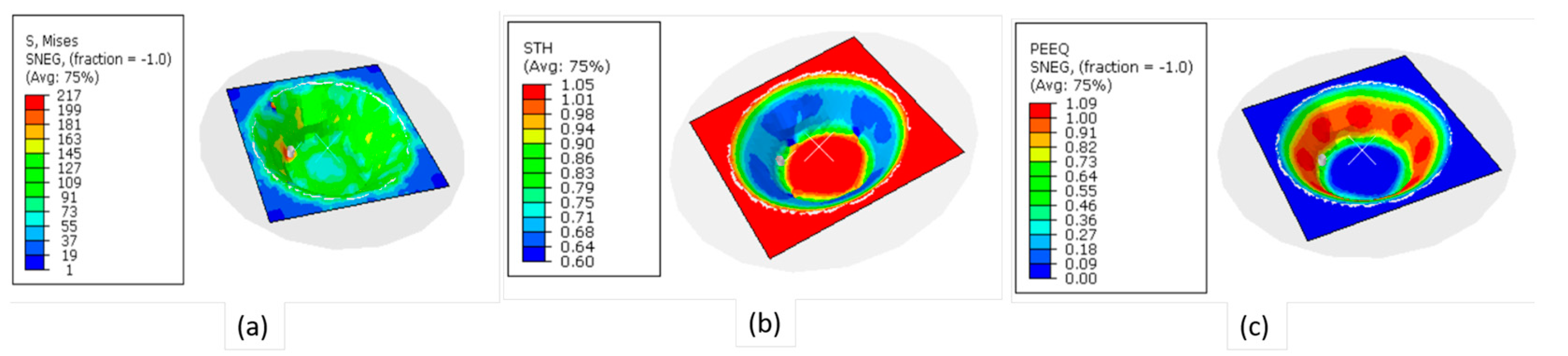The simulation was run, and dynamic analysis was done for stresses, strains, and tool forces arising during the tool motion, the results of which are given in Figure 7.

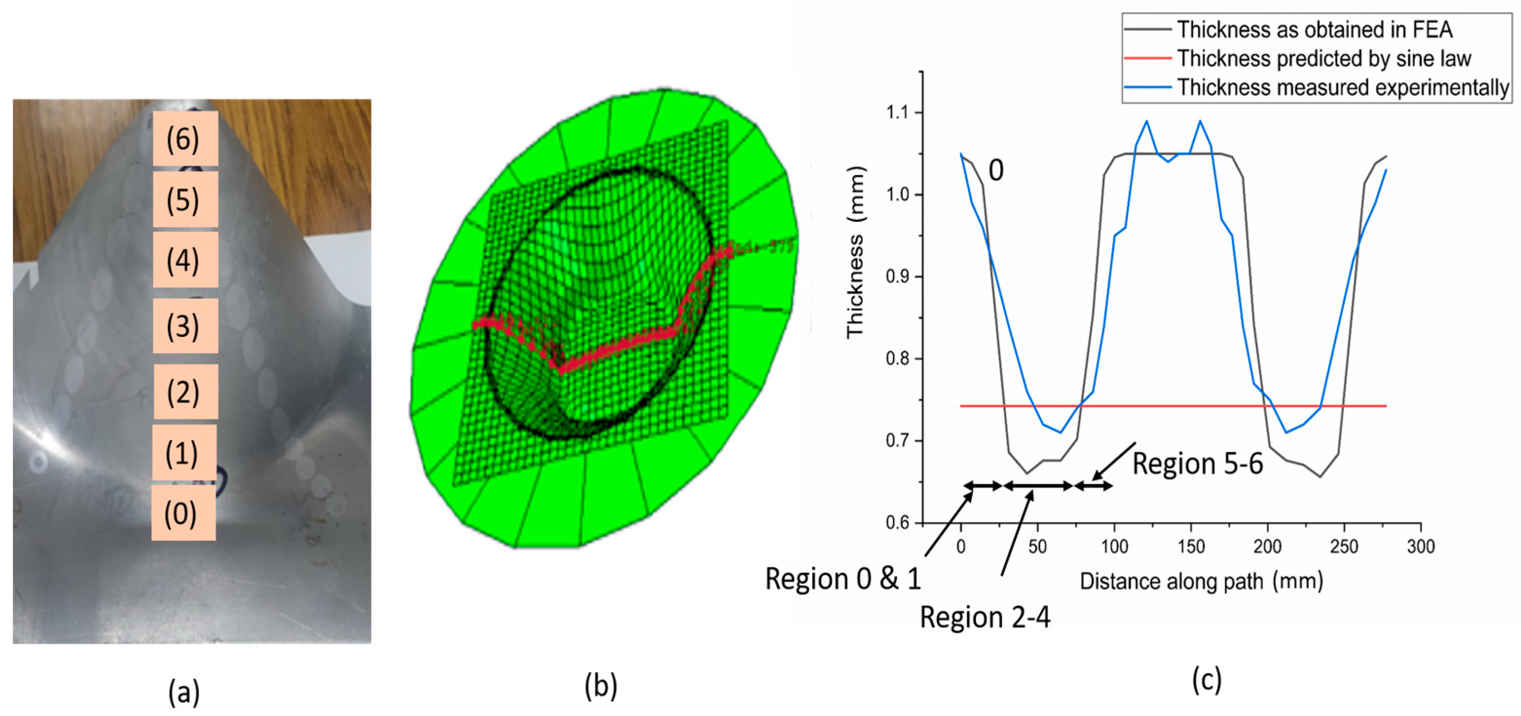
As can be seen from Figure 7a, the Von-Mises stress is maximum in the direct contact region between the undeformed sheet and the tool. The middle region of the cone is strained to the maximum value, as can be seen in Figure 7b. 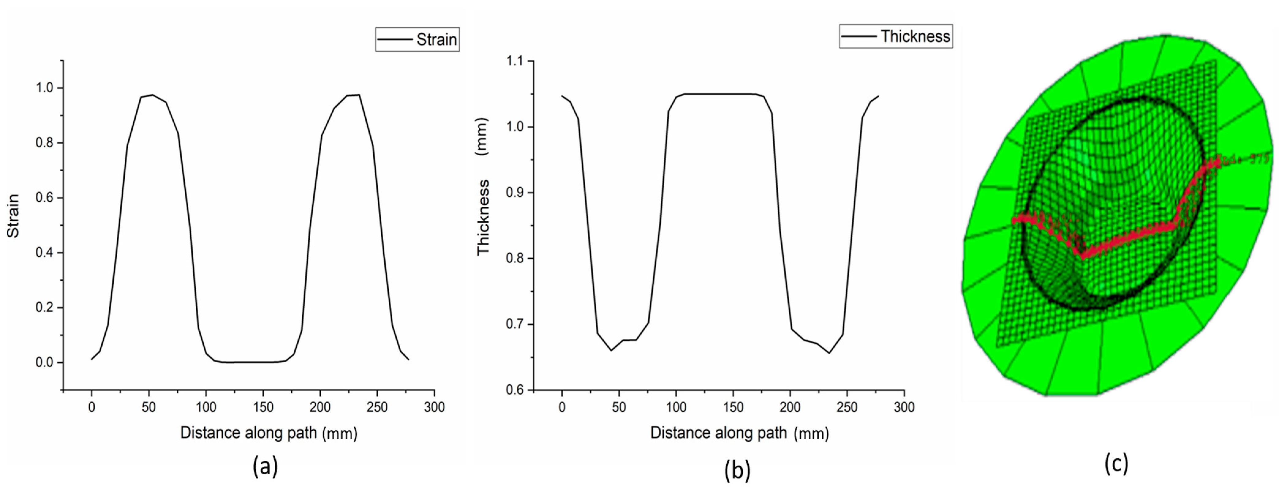Further, it can also be seen from Figure 7c that the middle region of the cone has the minimum thickness showing that this region has undergone the maximum amount of thinning, which also affirms the distribution as seen in Figure 7b. A path along the central meridional plane was chosen in the cone after deformation and strain occurred along the path, and the thickness of the sheet along the path was plotted, which is shown in Figure 8a,b.

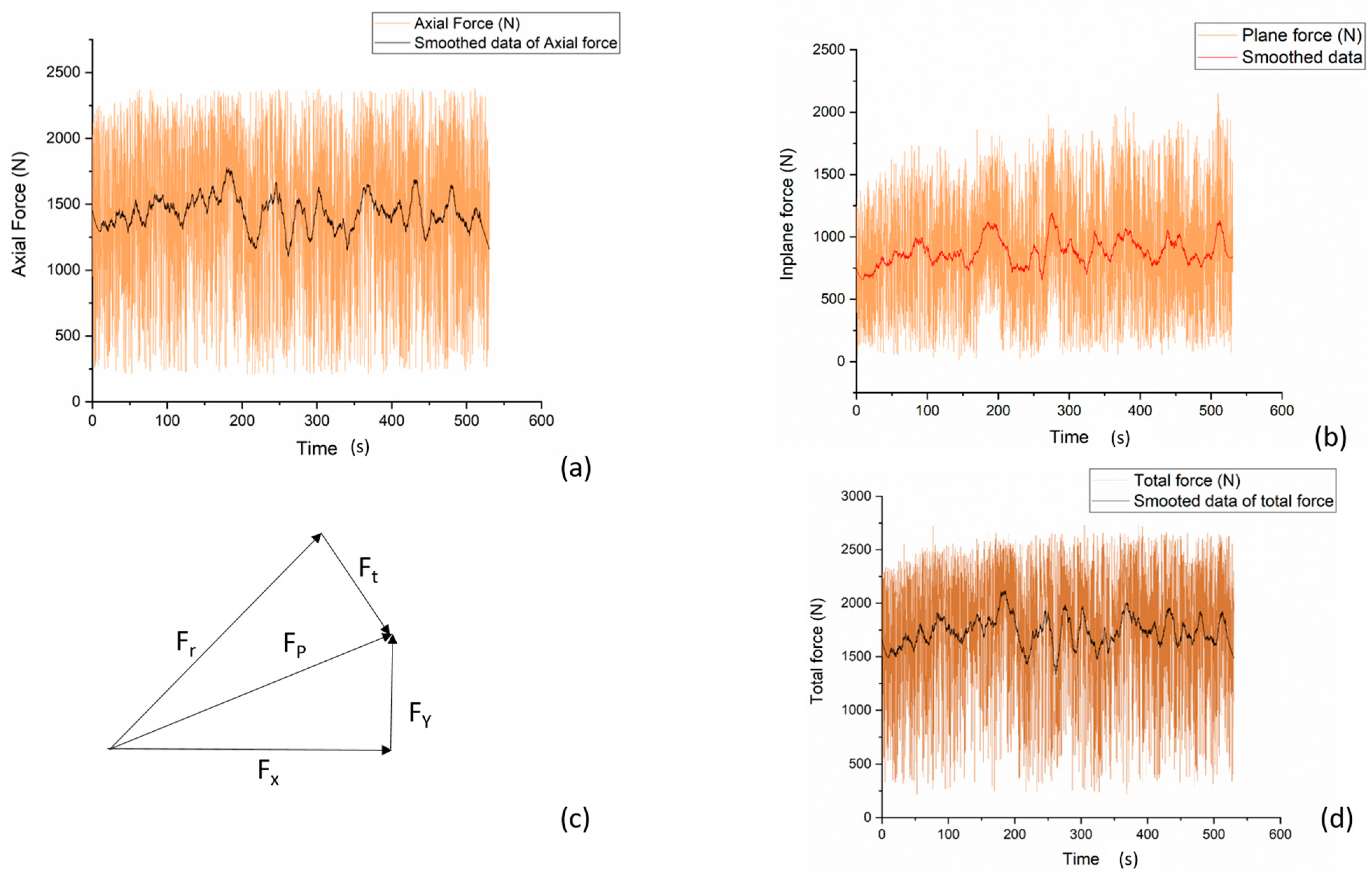
The simulation analysis was used to find out the forces appearing on the tool during the deformation. The tool force has been assumed to have two components. The axial components of the force F_zz and the resultant of in-plane X and Y components of forces is also equal to the resultant of tangential and radial force components.

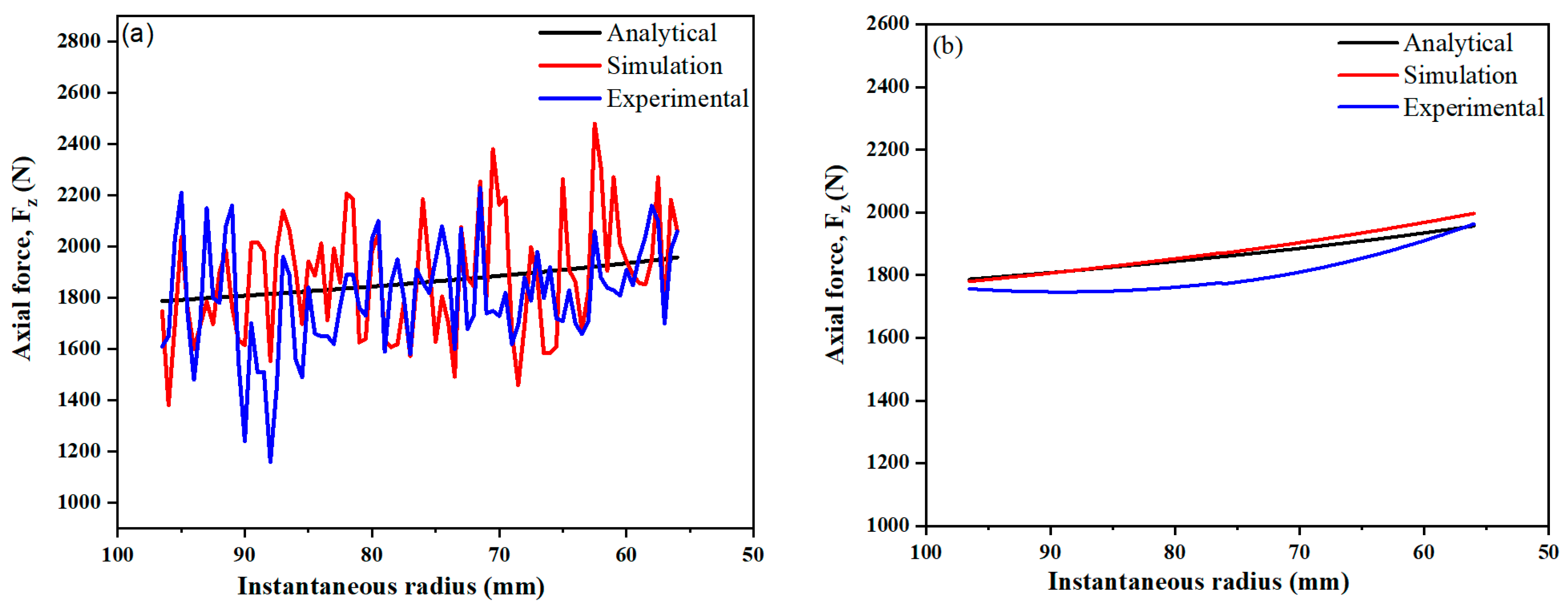
As can be seen from Figure 9, the largest force component arising during the deformation is in the axial direction, as was reported by Duflou et al. [20] as well. Additionally, it was observed that the largest axial force appearing in the axial direction was found to be 2629.11 N. The mean force was found to be 1512.24 N. The variation of in-plane force, that is, the resultant of the forces appearing in the plane of the undeformed sheet with time, has been shown in Figure 9b, and the force diagram for the same has been given in Figure 9c. The largest value corresponding to in-plane forming force was found to be 2172.31 N, and the average force during forming was found to be 1109.3 N. Finally, the variation of total forming force with time has been given in Figure 9d. The maximum forming force appearing on the tool was found to be 2747.46 N, and the average tool force was found to be 1812 N.

5. Experimental Validation

Once the analytical model was developed and force calculations were done, a simulation was carried out for preliminary validation of obtained forces analytically. Finally, experiments were carried out on a six-axis industrial robotic arm. 1.05 mm thick aluminum 6061 alloy sheets were taken for experimentation. The material composition is given in

Table 2. Chemical composition of 6061 Al alloy sheet used for experiments (wt%).

Elements	Al	Si	Fe	Zn	Cu	Cr	Mn	Mg	Ti
wt%	97.350	0.510	0.410	0.060	0.490	0.051	0.020	0.950	0.050

.

Tensile tests and Erichsen cup tests were carried out for the determination of material properties before conducting the experiments. The sample was considered to be isotropic. The tensile test was carried out on the 100 kN INSTRON 8801 model. ASTM/E8/E8M standards were followed for the making of the specimens [36]. The sample after the test is shown in Figure 10.

Once the test was conducted, the results were calculated using the data obtained from the test, which are summarized in

Table 3. Tensile properties of 6061 Al sheet.

Properties	Corresponding Values
Young’s modulus (GPa)	69.4
Yield strength (MPa)	111.6
Ultimate tensile strength (MPa)	118.2
Strain hardening exponent	0.2
Strength coefficient (MPa)	205

.

Before selecting a material, it is very crucial to have an idea of its formability. For the formability prediction of the sheet to be formed, the Erichsen cup test setup was used. The diameter of the used indenter was 20 mm. The main scale division was 1 mm, and the circular scale division was 50/5 MSD. The measured depth (H_E) for all the domes was measured, which is given in

Table 4. Data obtained from the Erichsen cup test.

Parameters	Al6061
	Dome 1	Dome 2	Dome 3
Measured depth (HE)	9.34	9.12	8.92
Dome height (Hd)	9.02	8.82	8.61
Average value of HE	9.13
Average value of Hd	8.81

. The domes are made as a result of indentation made by the indenter, as shown in Figure 11.

After obtaining the mechanical parameters from the uniaxial tensile test and Erichsen cup test, experiments were performed for which the chosen parameters are given in

Table 5. Various parameters used for forming the axis-symmetric cone.

Parameters	Corresponding Values
Tool speed	200 mm/s
Tool diameter	10 mm
Step depth	0.5 mm
Initial circle radius	96 mm
No. of cycles run	100
Measured depth of cone	47.6 mm
%ge spring back	4.8%

. The parameters were obtained using surface regression models. Dimension of the undeformed workpiece was taken as 250 mm × 250 mm × 1.05 mm. The sheet was deformed into a cone with a radius of the top circle 96 mm. The whole setup, the forming tool with the tool dynamometer, and the deformed axis-symmetric cone are shown in Figure 12a–c.

6. Results and Discussion

6.1. Thickness Distribution

The instantaneous thickness has a role to play in Equation (18). Hence the state of stress and the force are affected by the instantaneous sheet thickness, so the value of the sheet thickness was obtained from the FEA model and was validated by measuring the values after the experiments.

Once the experiments had been carried out, the thickness of the sheet was measured. The measurement was done by a micrometer with conical tips of least count 0.001 mm. The sheet was found to have the minimum thickness in the middle of the cone. The trend was also shown in previous work by Ambrogio et al. [37], who showed that the thickness prediction by the sine law is most accurate in the middle region of the deformed sheet. The conical region was divided into seven sub-regions (0–6), as shown in Figure 13a, and the thickness in the different regions was measured. Region-0 is the un-deformed region where thickness is 1.05 mm, and Region-6 is the region where the material gets accumulated because the tool moving along the sheet drags the material with it, and finally, it gets accumulated in the lowest region of the sheet; hence, the sheet thickness exceeds the original sheet thickness. However, Region-1–5 is the region in which sheet thinning occurs. The thickness plot for ISF in FEA and experiments are given in Figure 13c. For thickness prediction using FEA analysis, a path was chosen in the meridional direction, as shown in Figure 13b. The thickness variation obtained from FEA is shown in Figure 13c. All three thickness variations, obtained experimentally by FEA and by sine law [4], are plotted along the meridional path, as shown in Figure 13.

Force Measurement

For the measurement of forces, the cone was divided into seven zones. Zone 0 was taken as the zone of the upper undeformed cone, the middle region was taken as Zones 1–5 in which near uniform thinning occurs, and the sheet thinning followed the sine law, and Zone 6 was the region between the lower undeformed sheet and the cone, as shown in Figure 13a. The force was measured during deformation using a drill tool dynamometer. The setup is shown in Figure 12a,b. The capacity of the dynamometer is 500 kgf having a strain gauge based 350 Ω bridge sensor. The force was measured in X, Y, and Z directions, and the resultant of the forces in X and Y directions was calculated. Three forces were defined as F_z, F_p (resultant of forces in X and Y directions), and total force (F_t). Average values of F_z, F_p, and F_t were calculated for one complete cycle and were compared with the values obtained analytically. For comparison with the forces obtained from ABAQUS analysis, the average of forces for one complete circular cycle was calculated. Thus, all the components of forces were obtained from the analytical model, as well as the FEA model, using ABAQUS, and final validation was done by experimental results. The corresponding values of forces were plotted against the values of the instantaneous radius of the cone.

6.2. Variation of Axial Force

This force acts in the vertical direction. The force was calculated via an analytical model as well as the FEA model. Both were validated using final experimentation. The peak and the average value of the axial forces obtained in all three cases are given in

Table 6. Comparison of peak forces and average forces obtained analytically, by FEA model, and determined experimentally.

Model	Average Value (N)	Peak Value (N)
Analytical	1863.45	1957.15
FEA	1876.69	1997.01
Experimentation	1802.21	1963.41

.

The axial force increased with decreasing radius, as observed in the analytical model. The force in the axial direction is given by $F_{zz}={\sigma }_{zz}{A}_z+z_{rz}{A}_r$. The values of forces were calculated for different radii of the undeformed sheet using the formula, and the force was found to increase with the decreasing radius. The variation of the axial force with decreasing radii was almost linear. The same trend was seen in the FEA model, and experimentally, it was seen to increase with decreasing radii, but the shape of the plot departed from linearity slightly in the middle zone, as shown in Figure 14a,b. This can be due to sheet thinning, which can give rise to inaccurate sheet thickness at different points for a given radius. Nevertheless, the model gives a very good approximation of axial forming force during deformation. The error function for the error of the forces obtained analytically was defined as

$$\mathrm{Percentage}\mathrm{error}=\frac{{\mathrm{F}}_{\mathrm{analytical}}-{\mathrm{F}}_{\mathrm{experimental}}}{{\mathrm{F}}_{\mathrm{experimental}}}\times 100$$

(51)

The maximum error was found to be 4.92%. The force trends, as observed in ABAQUS, also closely matched the data obtained experimentally. The maximum error obtained in this case was 5.52%. The error in the axial force with respect to the experimental force calculated at every value of radius is shown in Section 6.4.

6.3. Variation of Resultant Force in r-θ Plane

The force in the r-θ plane has two components. For the mathematical model, the two components of forces evaluated were the ones in the r and θ planes. However, the components of the forces measured by the dynamometer and the forces observed in the ABAQUS analysis are in X and Y directions. So, the resultant of F_r and F_θ was calculated, which was equal to the resultant of F_X and F_Y. Finally, the force obtained analytically, and that obtained in FEA was compared with the experimental force. The peak and the average value of the resultant force in r-θ obtained in all three cases are given in

Table 7. Comparison of peak and average forces resultant force in r-θ plane obtained analytically, by FEA model, and determined experimentally.

Model	Average Value (N)	Peak Value (N)
Analytical	1538.63	1597.54
FEA	1526.26	1570.94
Experimentation	1493.88	1509.53

.

The plot of forces obtained in the r-θ plane from the analytical model, FEA, and experiment is given in Figure 15. The force obtained analytically had a good level of accuracy with experimental force. The largest error was found to be 8.47%, and the force obtained on FEA was found to have a maximum deviation of 4.61% from the values measured experimentally. The error in the axial force with respect to the experimental force calculated at every value of radius is shown in Section 6.4.

6.4. Variation of Total Force

In the analytical model, the total force appearing on the forming tool-sheet interface was calculated by the formula $F_t=\sqrt{{F_p}^2+{F_z}^2}$. Once the force was calculated, it was compared with the total force obtained experimentally and the one obtained in the FEA model. The peak and the average value of the total force obtained in all three cases are given in

Table 8. Comparison of peak and average value of total forces obtained analytically, by FEA model, and determined experimentally.

Model	Average Value (N)	Peak Value (N)
Analytical	2416.70	2504.13
FEA	1526.26	1570.94
Experimentation	1493.88	1509.53

.

The plot of total force obtained analytically, by the FEA model, and experimentally is given in Figure 16. The computed axial force from the mathematical model has a good level of accuracy as far as the total force is concerned. The maximum error in the calculated force from the total experimental force was found to be 4.25%.

The total force was also obtained from the FEA model on ABAQUS. The force obtained from the FEA model was also in close agreement with the total force obtained experimentally. The maximum error in obtained total force in the FEA model from the experimental model was found to be 4.89%, as shown in Figure 17c.

6.5. Error in Calculated and Experimentally Determined Forces

The forces calculated from the analytical model were compared with forces obtained by the FEA model and experimentally. For validation purposes, the true value of force was taken as the one which was obtained experimentally. The values of the forces were obtained from the analytical model for different instantaneous radii, and the corresponding values of the forces were also obtained from ABAQUS data. Both the values were compared with experimental values. So, validation of the mathematical model was done by comparing the values of the forces with the experimental values.

$$\mathrm{The}\mathrm{error}\mathrm{function}\mathrm{was}\mathrm{defined}\mathrm{as}\mathrm{percentage}\mathrm{error}=\frac{{\mathrm{F}}_{\mathrm{calculated}}-{\mathrm{F}}_{\mathrm{experimental}}}{{\mathrm{F}}_{\mathrm{experimental}}}\times 100$$

For axial forces and the total forces, the error was maximized in Zone 2, i.e., the middle region of the cone. However, for the resultant force in the r-θ plane, the error was maximum in Region-1, which decreased, and then the error was increased in Region-2 before finally decreasing in Region-3.

As far as the FEA model is concerned, the validation was done by comparing the forces obtained experimentally. The error for all three forces followed the same trend. The percentage error vs. instantaneous radius followed a bell curve pattern. It was maximized in Region-2 and was minimal in Region-1 and Region-3. The error curves are given in Figure 17a–c.

7. Conclusions

This paper presents an analytical model to predict the forming forces during incremental sheet forming. The modeling was done in a polar 3D coordinate system. All six stress components were taken into consideration initially before neglecting ${\tau }_{\theta z}$. Analytical formulae were developed for all the stress components. The contact area was modeled analytically before finally developing the equations for all forces. The three force components for which the equations were developed were F_r, F_θ, and F_z. The result of the three components is the total force F_t. The resultant of F_r and F_θ is the resultant force in the r-θ plane, represented as F_p. The material used in the mathematical model was AA6061. The process was modeled in FEA using the same experimental parameters, and the force components F_z and F_p were calculated before finally calculating the total force (F_t). Finally, the process was carried out on a six-axis industrial robot, and forces were measured using a tool dynamometer. The data obtained from the analytical model and FEA were validated by the experimental results. The model is for all wall angle cones; however, in this work, the validation has been done for a 45° cone. The results obtained from the analytical model and FEA were in good agreement with the experimental result. The maximum error in the analytically calculated total force was found to be 4.25%. Similarly, the results obtained from the FEA model were also in agreement with the experimental results. The maximum error in evaluated total force from the FEA model was found to be 4.89% with respect to the experimental results. It can be concluded that the mathematical model developed can be used for a force calculation to a good level of accuracy.

References

1. Edward, L. Apparatus and Process for Incremental Dieless Forming. U.S. Patent 3,342,051, 19 September 1967. [Google Scholar]
2. Jeswiet, J.; Micari, F.; Hirt, G.; Bramley, A.; Duflou, J.; Allwood, J. Asymmetric Single Point Incremental Forming of Sheet Metal. CIRP Ann. 2005, 54, 88–114. [Google Scholar] [CrossRef]
3. Iseki, H. Flexible and incremental sheet metal bulging using a few spherical rollers. Trans. Jpn. Soc. Mech. Eng. 1993, 59, 2849. [Google Scholar] [CrossRef]
4. Kim, T.; Yang, D.-Y. Improvement of formability for the incremental sheet metal forming process. Int. J. Mech. Sci. 2000, 42, 1271–1286. [Google Scholar] [CrossRef]
5. Shim, M.-S.; Park, J.-J. The formability of aluminum sheet in incremental forming. J. Mater. Process. Technol. 2001, 113, 654–658. [Google Scholar] [CrossRef]
6. Kim, Y.H.; Park, J.J. Effect of process parameters on formability in incremental forming of sheet metal. J. Mater. Process. Technol. 2002, 130, 42–46. [Google Scholar] [CrossRef]
7. Avitzur, B.; Yang, C. Analysis of power spinning of cones. J. Eng. Ind. Aug. 1960, 82, 231–244. [Google Scholar] [CrossRef]
8. Kim, J.H.; Park, J.H.; Kim, C. A Study on the mechanics of shear spinning of cones. J. Mech. Sci. Technol. 2006, 20, 806–818. [Google Scholar] [CrossRef]
9. Jackson, K.; Allwood, J.; Landert, M. Incremental forming of sandwich panels. J. Mater. Process. Technol. 2008, 204, 290–303. [Google Scholar] [CrossRef]
10. Kalpakcioglu, S. On the Mechanics of Shear Spinning. J. Eng. Ind. 1961, 83, 125–130. [Google Scholar] [CrossRef]
11. Jackson, K.; Allwood, J. The mechanics of incremental sheet forming. J. Mater. Process. Technol. 2009, 209, 1158–1174. [Google Scholar] [CrossRef]
12. Ma, L.; Wang, Z. The effects of through-thickness shear stress on the formability of sheet metal—A review. J. Manuf. Process. 2021, 71, 269–289. [Google Scholar] [CrossRef]
13. Allwood, J.M.; Shouler, D.R. Generalised forming limit diagrams showing increased forming limits with non-planar stress states. Int. J. Plast. 2009, 25, 1207–1230. [Google Scholar] [CrossRef]
14. Emmens, W.; Boogaard, A.V.D. An overview of stabilizing deformation mechanisms in incremental sheet forming. J. Mater. Process. Technol. 2009, 209, 3688–3695. [Google Scholar] [CrossRef]
15. Emmens, W.; Boogaard, A.V.D. Incremental forming by continuous bending under tension—An experimental investigation. J. Mater. Process. Technol. 2009, 209, 5456–5463. [Google Scholar] [CrossRef]
16. Eyckens, P.; Van Bael, A.; Aerens, R.; Duflou, J.; Van Houtte, P. Small-scale Finite Element Modelling of the Plastic Deformation Zone in the Incremental Forming Process. Int. J. Mater. Form. 2008, 1, 1159–1162. [Google Scholar] [CrossRef]
17. Sawada, T.; Fukuhara, G.; Sakamoto, M. Deformation mechanism of sheet metal in stretch forming with computer numerical control machine tools. J. Jpn. Soc. Technol. Plast. 2001, 42, 1067–1069. [Google Scholar]
18. Li, Y.; Daniel, W.J.T.; Meehan, P.A. Deformation analysis in single-point incremental forming through finite element simulation. Int. J. Adv. Manuf. Technol. 2017, 88, 255–267. [Google Scholar] [CrossRef]
19. Kumar, A.; Gulati, V.; Kumar, P.; Singh, H. Forming force in incremental sheet forming: A comparative analysis of the state of the art. J. Braz. Soc. Mech. Sci. Eng. 2019, 41, 251. [Google Scholar] [CrossRef]
20. Duflou, J.R.; Tunckol, Y.; Aerens, R. Force Analysis for Single Point Incremental Forming. Key Eng. Mater. 2007, 344, 543–550. [Google Scholar] [CrossRef]
21. Aerens, R.; Eyckens, P.; Van Bael, A.; Duflou, J.R. Force prediction for single point incremental forming deduced from experimental and FEM observations. Int. J. Adv. Manuf. Technol. 2010, 46, 969–982. [Google Scholar] [CrossRef]
22. Saidi, B.; Boulila, A.; Ayadi, M.; Nasri, R. Experimental force measurements in single point incremental sheet forming SPIF. Mech. Ind. 2015, 16, 410. [Google Scholar] [CrossRef]
23. Jeswiet, J.; Duflou, J.R.; Szekeres, A. Forces in Single Point and Two Point Incremental Forming. Adv. Mater. Res. 2005, 6–8, 449–456. [Google Scholar] [CrossRef]
24. Xiao, X.; Kim, C.-I.; Lv, X.-D.; Hwang, T.-S.; Kim, Y.-S. Formability and forming force in incremental sheet forming of AA7075-T6 at different temperatures. J. Mech. Sci. Technol. 2019, 33, 3795–3802. [Google Scholar] [CrossRef]
25. Flores, P.; Duchêne, L.; Bouffioux, C.; Lelotte, T.; Henrard, C.; Pernin, N.; Van Bael, A.; He, S.; Duflou, J.; Habraken, A. Model identification and FE simulations: Effect of different yield loci and hardening laws in sheet forming. Int. J. Plast. 2007, 23, 420–449. [Google Scholar] [CrossRef]
26. Henrard, C.; Bouffioux, C.; Eyckens, P.; Soly, H.; Duflou, J.; Van Houtte, P.; Van Bael, A.; Duchêne, L.; Habraken, A. Forming forces in single point incremental forming: Prediction by finite element simulations, validation and sensitivity. Comput. Mech. 2011, 47, 573–590. [Google Scholar] [CrossRef]
27. Honarpisheh, M.; Keimasi, M.; Alinaghian, I. Numerical and experimental study on incremental forming process of Al/Cu bimetals: Influ-ence of process parameters on the forming force, dimensional accuracy and thickness variations. J. Mech. Mater. Struct. 2018, 13, 35–51. [Google Scholar] [CrossRef]
28. Iseki, H. An approximate deformation analysis and FEM analysis for the incremental bulging of sheet metal using a spherical roller. J. Mater. Process. Technol. 2001, 111, 150–154. [Google Scholar] [CrossRef]
29. Silva, M.; Skjoedt, M.; Martins, P.; Bay, N. Revisiting the fundamentals of single point incremental forming by means of membrane analysis. Int. J. Mach. Tools Manuf. 2008, 48, 73–83. [Google Scholar] [CrossRef]
30. Chang, Z.; Li, M.; Chen, J. Analytical modeling and experimental validation of the forming force in several typical incremental sheet forming processes. Int. J. Mach. Tools Manuf. 2019, 140, 62–76. [Google Scholar] [CrossRef]
31. Bansal, A.; Lingam, R.; Yadav, S.K.; Reddy, N.V. Prediction of forming forces in single point incremental forming. J. Manuf. Process. 2017, 28, 486–493. [Google Scholar] [CrossRef]
32. Fang, Y.; Lu, B.; Chen, J.; Xu, D.; Ou, H. Analytical and experimental investigations on deformation mechanism and fracture behavior in single point incremental forming. J. Mater. Process. Technol. 2014, 214, 1503–1515. [Google Scholar] [CrossRef]
33. Liu, F.; Li, Y.; Cheng, Z.; Wang, Z.; Li, F.; Li, J. Preliminary modelling of forming forces in three directions for incremental sheet forming process based on the contact area. Procedia Manuf. 2020, 50, 630–636. [Google Scholar] [CrossRef]
34. Liu, F.; Li, Y.; Yuan, H.; Sun, R.; Li, F.; Li, J. Comprehensive modeling of forming forces in three directions for incremental sheet forming process based on the contact area. J. Manuf. Process. 2022, 84, 986–1000. [Google Scholar] [CrossRef]
35. Dalir, M.A.; Seifi, R. Direct method for deriving equilibrium equations in solid continuous systems. Eng. Solid Mech. 2014, 2, 321–330. [Google Scholar] [CrossRef]
36. E8/E8M-16a; Standard Test Methods for Tension Testing of Metallic Materials. ASTM International: West Conshohocken, PA, USA, 2016.
37. Ambrogio, G.; Filice, L.; Gagliardi, F.; Micari, F. Sheet Thinning Prediction in Single Point Incremental Forming. Adv. Mater. Res. 2005, 6–8, 479–486. [Google Scholar] [CrossRef]
Figure 1. (a) Schematic diagram of ISF (b) Forming forces in the plane of an undeformed sheet (c) Vector diagram of forming forces in the plane of an undeformed sheet.
Processes 11 01688 g001
Figure 2. (a) Definition of the 3D polar coordinate for considering an element, and (b) representation of the taken element. (c) Definition of wall angle in terms of step depth. (d) Stresses acting on the taken element.
Processes 11 01688 g002
Figure 3. The process simulated under the same condition on ABAQUS: (a) the radial stress distribution at a radius of 82.5 mm and (b) the chosen path on the radial line for stress distribution.
Processes 11 01688 g003
Figure 4. (a) Three-dimensional view of the contact area, (b) contact area in rz plane, and (c) top view of (d) section XX′.
Processes 11 01688 g004
Figure 5. Parts used in ABAQUS with dimensions in mm (a) tool holder (b) sheet (c) forming tool [32].
Processes 11 01688 g005
Figure 6. Engineering and true stress and strain curve for Aluminum 6061 alloy.
Processes 11 01688 g006
Figure 7. Simulation results of formed part on ABAQUS: (a) stress distribution (MPa) in the deformed cone, (b) strain distribution in the deformed cone, and (c) thickness variation (mm) within the deformed cone.
Processes 11 01688 g007
Figure 8. (a) Strain vs. true distance along the path, (b) true thickness vs. true distance along the path, and (c) chosen path.
Processes 11 01688 g008
Figure 9. (a) Axial force with a smoothened curve, (b) in plane force with a smoothened curve, (c) decomposition of plane forces, and (d) total force with a smoothened curve.
Processes 11 01688 g009
Figure 10. (a) Setup for tensile testing, (b) sample under tension, and (c) tensile test sample.
Processes 11 01688 g010
Figure 11. Domes made after the Erichsen cup test.
Processes 11 01688 g011
Figure 12. (a) Setup with tool dynamometer, (b) tool used for sheet deformation, (c) deformed sheet.
Processes 11 01688 g012
Figure 13. (a) Different regions defined on the formed cone, (b) path chosen on formed cone in FEA model, and (c) thickness variation evaluated experimentally by FEA model and by sine law.
Processes 11 01688 g013
Figure 14. (a) Variation of axial force and (b) fit curve of axial force with the instantaneous radius of the undeformed sheet as observed from the mathematical model, FEA, and experiments.
Processes 11 01688 g014
Figure 15. (a) Variation of Fp and (b) fit curve of Fp with an instantaneous radius of the undeformed sheet as observed from the mathematical model, FEA, and experiments.
Processes 11 01688 g015
Figure 16. (a) Variation of total force and (b) fit curve of total force with an instantaneous radius of the undeformed sheet as observed from the mathematical model, FEA, and experiments.
Processes 11 01688 g016
Figure 17. Percentage error in (a) axial force, (b) resultant force, and (c) total force.
Processes 11 01688 g017