Article

Design of Photovoltaic Power Generation Servo System Based on Discrete Adaptive Network Dynamic Surface Control Technology

Yunnan Electric Power Grid Research Institute, Kunming 650217, China
*
Author to whom correspondence should be addressed.
Processes 2023, 11(6), 1667; https://doi.org/10.3390/pr11061667
Submission received: 4 April 2023 / Revised: 25 May 2023 / Accepted: 25 May 2023 / Published: 30 May 2023
(This article belongs to the Special Issue Photovoltaic (PV) Systems: Modelling, Measurement and Assessment)

Abstract

:
In recent years, under the development of the dual carbon goal, the energy crisis has become increasingly serious, and China has also experienced serious power rationing. However, the research on dynamic surface control technology in solar tracking systems in nonlinear control systems is mostly based on continuous-time systems, while adaptive dynamic surface control based on discrete-time nonlinear control systems can describe an actual control system more accurately in the production process. It can effectively suppress interference with extremely high stability and safety. To solve the problem of low efficiency in photovoltaic power generation, this research first built a photovoltaic power generation servo system model based on the parameter of uncertainty. Then, a discrete adaptive neural network dynamic surface (DANNDS) controller was designed to solve the problems in the design of the traditional backstepping method. Finally, based on the designed method of a dynamic surface controller, a discrete adaptive neural network quantization controller (DANNQC) for the photovoltaic power generation servo system was designed by introducing external disturbance. The control parameters and their studied ranges were as follows: The reference signals were o r 1 = sin ( 0.1 t ) and o r 2 = cos ( 0.1 t ) . The parameters of the virtual control law and the final control law were m 11 = 0.01 , m 22 = 0.01 , m 12 = 0.02 , m 13 = 0.02 , and m 23 = 0.02 . The time constant of the low-pass filter was ζ 12 = ζ 13 = ζ 22 = ζ 23 = 0.005 . The parameters of the parameter regulation law were ρ 12 = ρ 13 = ρ 22 = ρ 23 = 0.0005 and a 12 = a 13 = 20 , a 22 = a 23 = 22 . The research results show that the MTE, RMSTE, and 2NTE scores of the height angle servo motor of the DANNDS control method were 0.0026, 7.0279 × 10⁻⁴, and 0.3552, respectively. The scores for each index of the azimuth servo motor were 0.0028, 8.9237 × 10⁻⁴, and 0.4511, respectively. The height angle tracking error for the DANNQC control method was [−0.02,0.022]. The azimuth tracking error was [−0.03,0.03]. In summary, the photovoltaic power generation servo system based on the DANNQC has a better control performance. By controlling the height angle and azimuth angles, it can better track the position of the sun and adjust the position of the photovoltaic panel in real time. The sun’s rays illuminate the photovoltaic panel at an appropriate angle to achieve maximum power generation efficiency, which is of great practical significance for the development of solar technology.

1. Introduction

Energy is the foundation and driving force for the progress of human civilization. The national economy, people’s livelihoods, and national security are crucial for improving people’s well-being and promoting economic and social development [1]. However, in recent years, the demand for energy in human society has increased, and the energy problem has attracted the attention of people around the world. Although the use of energy has promoted economic growth in all countries, it also poses great challenges to mankind [2]. At present, there is very little research on the technology of energy transformation. Although the use of renewable energy can alleviate the energy crisis, its infrastructure construction is not advanced enough, which still causes China to experience large-scale power rationing [3]. In addition, human misuse of energy resources leads to an insufficient sustainable energy supply, resource shortage, ecological pollution, and other problems that seriously affect human survival and development [
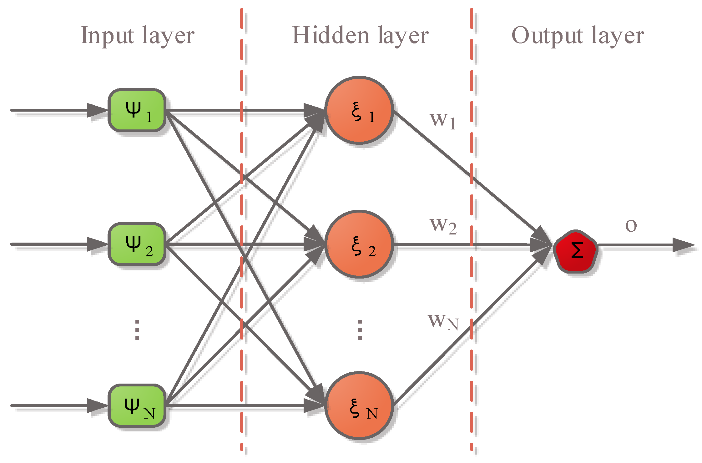
4]. A photovoltaic power generation servo system can track the position of the sun and adjust the position of the photovoltaic panel in real time, achieving maximum power generation efficiency by shining sunlight at an appropriate angle onto the photovoltaic panel. Servo motors can convert voltage signals into torque and speed to drive control objects, accurately controlling the position of the motor, and they are widely used in various fields. However, photovoltaic power generation servo control systems have many unknown parameters and complex controls, making it difficult to achieve precise tracking control. Therefore, how to improve the daily tracking progress of photovoltaic power generation systems is a widely concerning issue for many scholars. Dynamic surface (DS) control technology was developed based on backstepping technology, which overcomes the computational complexity of the traditional backstepping design and makes the controller and parameter design simpler. This technology can effectively reduce the number of input variables for neural networks and fuzzy systems used for modeling [5]. However, the research on DS technology in nonlinear control systems is mostly based on continuous-time systems, and there is less research on adaptive DS control technology based on discrete-time nonlinear control systems. The digital correction effect used in a discrete-time system is better than that in a continuous correction device. Its software is more convenient for the realization of control law modification, flexible control, and a more accurate description of the actual production process [6]. In addition, the information transmission in discrete-time control (DTC) systems can effectively suppress interference and have better stability [
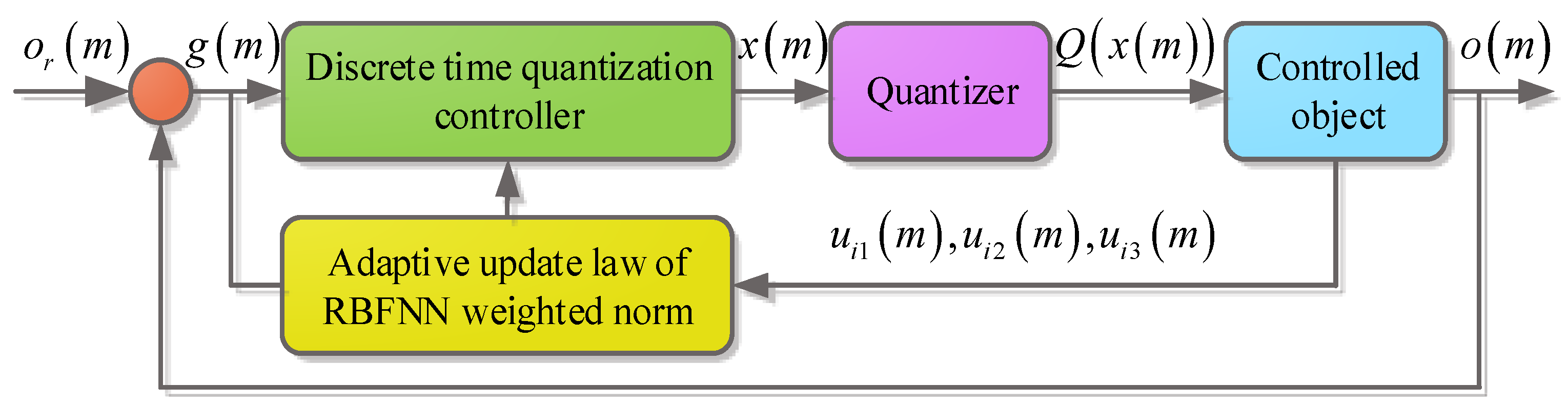
7]. In order to solve the problem of two-axis tracking in a photovoltaic power generation system and using adaptive DS technology based on a discrete-time system, a discrete adaptive neural network dynamic surface (DANNDS) controller was designed. Then, based on this DANNDS controller, a photovoltaic power generation servo system based on a discrete adaptive neural network quantization controller (DANNQC) was established in this research.
This research aims to improve the tracking efficiency of solar power generation systems and better develop new energy power generation so as to make it correspond to the goal of carbon neutrality and carbon peak shaving. In addition, the application fields for DS control technology are very extensive, and currently, there are related applications in power systems, aircraft control, and the shipbuilding industry. The research on DS control technology can further promote its development. Finally, most of the research on DS control technology in nonlinear control systems is based on continuous-time systems. The adaptive DS control of discrete-time nonlinear control systems proposed in this study can provide more accurate descriptions of actual control systems in the production process and can effectively suppress drying. Its stability and safety are extremely high, which can increase the development of nonlinear control fields and have important practical significance. The innovation points of this research are as follows: the first point is to propose an adaptive dynamic surface control scheme based on discrete systems, and the second point is to design an adaptive neural network tracking control scheme with state quantization considering the uncertainty of system parameters and external disturbances.

2. Related Work

A photovoltaic power generation servo system realizes the tracking control of a solar track by simultaneously controlling the height angle motor and the azimuth angle motor. The two servo systems in the system are the same and independent of each other [8]. Servo motor control has important practical significance for improving the control and tracking accuracy of photovoltaic power generation servo systems and ensuring the safe and stable operation of power systems [9]. However, a photovoltaic power generation servo control system has many unknown parameters, and the control is complex. It is difficult to achieve accurate tracking control. Therefore, many scholars have conducted in-depth discussions about photovoltaic power generation systems and improving the sun-seeking accuracy of photovoltaic power generation systems. In order to improve the power quality of a three-phase power system, Panigrahi et al. designed a model using a multi-level inverter to optimize a photovoltaic microgrid to improve the power quality. The research showed that the model was helpful for managing reactive power by controlling the direct current (DC) bus voltage through the photovoltaic system, and it also helped to reduce harmonics and provide additional active power to the load in case of electrical interference on the grid side [10]. Mathivanan proposed using an appropriate controller in a solar photovoltaic flywheel energy storage system for new energy storage and power regulation. The flywheel is responsible for the dynamic stability of the system, and the reliability of the system is guaranteed with a good controller unit. The solar photovoltaic power generation device and its controller were simulated and tested using MATLAB software, and the results verified the performance of the system [11]. To achieve reliable power system dispatching, Mei et al. built a set of non-parametric probability prediction models for photovoltaic power generation. The quantile regression average was used to integrate a group of independent long-term and short-term deterministic prediction models to obtain the probability prediction of the PV output. Experimental data verified the effectiveness of the model. Compared with the benchmark method, the proposed method has better prediction performance [12]. Shi et al. designed a high-gain soft-switching boost CLLC converter with PWM and pulse frequency modulation hybrid modulation control for photovoltaic power generation in order to maximize the energy generated with the photovoltaic power generation system and improve the conversion efficiency. They verified the efficiency of the converter and the feasibility of this method through experiments [13].
A solar tracking system is widely used in solar photovoltaic applications. It is an electrical device that allows a solar panel to always face the sun so that the sunlight always shines in a vertical direction on the solar panel. However, the tracker in solar tracking systems has a shorter lifespan and lower reliability, so many scholars have conducted in-depth discussions. Umer et al. proposed an extended TOPSIS technology based on interval type-II Pythagorean fuzzy numbers for the efficient utilization of solar energy and applied this technology to solar tracking systems. The experimental results showed that the performance of the solar tracking system applied to TOPSIS technology was superior [14]. Saeedi M. et al. designed a double-axis solar tracker based on a Wheatstone bridge circuit and LDR sensor to improve the output power of photovoltaic panels. The simulation results confirmed that the output power of the photovoltaic panel using a biaxial solar tracker was higher than that of the fixed panel [15]. Anuraj et al. discussed the design of a solar tracking system using a stepper motor based on LDR sensors and an ATMaga16 microcontroller to reduce the initial cost of establishing a solar tracking system. The research results indicated that the system achieved precise automatic tracking of the sun [16]. Fb et al. selected phase change materials, thermoelectric materials, and aluminum fins to cool the photovoltaic panels of solar tracking systems using different cooling methods, and they compared the surface temperatures and output powers of the photovoltaic panels. Simulation experiments demonstrated that under the same environmental conditions, using aluminum fins as the cooling method for the photovoltaic panels of the solar tracking system could effectively reduce the surface temperature of the panels and increase the output power [17]. Bashar designed a solar dual tracking system with intelligent power and tracking performance data monitoring to improve the efficiency of photovoltaic panels. Through the test results of the system at different time periods, it is known that the dual tracking system has good feasibility [18]. Abir Muntacir et al. constructed a self-powered dual-axis tracking system for solar panels based on Arduino controllers to address the growing demand for electricity. The system always maintains the alignment of solar panels with the sun for energy regeneration. When the light intensity decreases due to changes in the position of the sun, the system automatically changes direction to achieve the maximum light intensity. Simulation experiments have proven that this system can improve the utilization efficiency of photovoltaic panels or any solar energy device [19].
To sum up, there are many research results about photovoltaic power generation systems and nonlinear control technology, but there is relatively little research on adaptive DS control based on a discrete-time nonlinear control system. For solving the efficiency problem of photovoltaic power generation systems and how to combine DS technology with photovoltaic power generation systems, a DANNDS controller and a photovoltaic power generation servo system based on a DANNQC were proposed.

3. Design of Photovoltaic Power Generation Servo System Based on DANNQC

3.1. Modeling Pretreatment of Photovoltaic Power Generation Servo System Based on DANNQC

A photovoltaic power generation servo system is an automatic control system, and its stability is the most important aspect. Lyapunov stability (LS) [20] is the most widely used method to judge the stability of systems. LS theory is used to describe the stability of a dynamic system. If the trajectory of the dynamic system near the equilibrium state can be maintained near the equilibrium state under any initial condition, it is Lyapunov stable. If the trajectory of any initial condition near the equilibrium finally approaches it, the system is said to be asymptotically stable. Global asymptotic stability is when all non-zeros in the state space are taken as initial perturbations, and the perturbed motion system is asymptotically stable. This is the most desirable feature of a system in control engineering. The necessary condition for a system to not be globally asymptotically stable is only having one equilibrium state in the state space. If there is a selected sphere, no matter how small the radius of the sphere is, there is always at least one point in the sphere. If the perturbed motion trajectory starting from this state is separated from the sphere, the system origin equilibrium state is said to be unstable. In classical control theory, only asymptotically stable systems are considered stable systems. A system that is stable only in the Lyapunov sense but is not asymptotically stable is called a critically stable system, which is unstable in engineering. Considering a DTC system, the difference equation is as follows (1).
{ u ( m + 1 ) = f ( m , u ( m ) ) f ( m , 0 ) = 0 m N
u ( m ) in Equation (1) represents the state variable of the system. f ( m , u ( m ) ) is a N -dimensional vector function. Letting u ( m ) be the solution sequence of Equation (1), Equation (2) can then be obtained.
Δ V ( m , u ( m ) ) = V ( m + 1 , f ( m , u ( m ) ) ) V ( m , u ( m ) )
Equation (2) is the difference of the solution of function V ( m , u ( m ) ) via Equation (1). In the design of a DTC system, the traditional backstepping control method needs to multiple differential calculations on the virtual controller. As the order of the system increases, the order of the difference also increases. The designed virtual controller contains information about the future time, which will cause non-causal problems and then cause the virtual controller to fail. In order to solve the problem of the traditional backstepping control method, the DS control method introduces a first-order low-pass filter to avoid the complex system model from being converted into a special form. This simplifies the design of controllers and parameters [21]. Equation (3) is the DS controller of the DTC system.
{ a i ( m + 1 ) = b i ( a ¯ i ( m ) ) a i + 1 ( m ) + f i ( a ¯ i ( m ) ) , i = 1 , 2 , , n 1 a n ( m + 1 ) = b n ( a ¯ n ( m ) ) x ( m ) + f n ( a ¯ n ( m ) ) o ( m ) = a 1 ( m )
a ¯ i ( m ) = [ a 1 ( m ) , a 2 ( m ) , , a i ( m ) ] T R i in Equation (3) is the state variable of the system. x ( m ) and o ( m ) are the control inputs and outputs of the system. b i ( a ¯ i ( m ) ) and f i ( a ¯ i ( m ) ) are unknown nonlinear functions in the system. The control objective is to assume that a d ( m ) is a smooth function. Through the control design, o ( m ) can continuously track the desired signal o r ( m ) . The design steps of the DS controller of the DTC system are as follows: first, defining the first error surface g 1 ( m ) ; designing the virtual control law u 1 ( m ) ; and letting g 1 ( m ) pass through a low-pass filter. Eventually, a new state variable u 1 d ( m ) can be obtained. See Equation (4) for the calculation.
{ u 1 d ( m ) + ζ f 1 u 1 d ( m + 1 ) = u 1 ( m ) u 1 d ( 0 ) = u 1 ( 0 )
In Equation (4) of ζ f 1 = ζ 1 Δ t , ζ 1 is the time constant. Then, the above steps are repeated until the n -th error surface g n ( m ) is defined. Letting u n 1 ( m ) pass through a low-pass filter to obtain a new state variable u ( n 1 ) d ( m ) , the final actual control law is then obtained as calculated using Equation (5).
u ( m ) = f n ( a ¯ n ( m ) ) u n 1 ( m + 1 ) b n ( a ¯ n ( m ) )
Due to the introduction of a first-order low-pass filter, the problem of filtering error o i ( m ) arises. The calculation of o i ( m ) is shown in Equation (6).
o i ( m ) = u i d ( m ) u i ( m )
When analyzing the stability of the Lyapunov function, o i ( m ) needs to be considered. The problem in the design of the above DTC system is that linear partitioning is not possible. A radial basis function neural network (RBFNN) can approach any nonlinear function, has an excellent generalization ability and learning speed, and easily deals with the problem of impossible linear partitioning in low dimensions [22]. The principle of an RBFNN is as follows. By using the radial basis function as the activation function of a neural network, the neural network can map the input data nonlinearly and better adapt to the complex relationships within or between the data. Compared with traditional activation functions such as sigmoid and ReLU, the radial basis function has better smoothness and locality so it can better fit the local characteristics of data. This outer diameter basis function also has good scalability and interpretability, which can provide interpretability for the output of a neural network and aid in the decision-making process of the neural network. The structure of an RBFNN is shown in Figure 1.
In Figure 1, the RBFNN is a three-layer forward network from the input layer, the hidden layer, to the output layer. ψ = [ ψ 1 , ψ 2 , , ψ N , ] T R N is the input of the network. ξ = [ ξ 1 , ξ 2 , , ζ N , ] T R N represents the output of the hidden layer. W = [ w 1 , w 2 , , w N , ] T R N represents the weight vector of the network. o R is the output of the network. The output calculation of the j -th neuron in the hidden layer is shown in Equation (7).
ξ j ( ψ ) = exp ( ψ c j 2 2 h j 2 )
In Equation (7), c j and h j represent the center vector and width of the j -th basis function, respectively, and the basis function is a Gaussian function. The final output of the RBFNN is shown in Equation (8).
o j = i = 1 a w i j exp ( 1 2 β 2 u p c i ) , j = 1 , 2 , , n
β in Equation (8) represents the Gaussian function. The training methods of the RBFNN are mainly divided into two categories: linear least squares (LLS) and orthogonal least squares (OLS). The LLS method can minimize the sum of squares of errors between the output and input of the network. The OLS rule is to construct an orthogonal matrix by rotating the input and output coordinate systems into mutually orthogonal coordinate systems and then use the least squares method to solve the eigenvectors and eigenvalues of the matrix. By selecting the least squares solution to train the neural network, the ideal model output can be obtained. Although the computational complexity of the OLS method can further improve the stability and generalization ability of neural network models compared with the LLS method, this study chose the OLS method as the training method for the RBFNN. The control system used in this study is a DTC system. The signal between the controller and the system is transmitted through the network medium with limited bandwidth. The transmission of digital signals is not limited by broadband and can effectively suppress noise, optimizing the anti-interference performance of the DTC system [23]. At present, the commonly used non-uniform quantizers include the hysteresis quantizer and the logarithmic quantizer. The logarithmic quantizer can quantize signals of different sizes with different quantization intervals. This makes the system need less information to reach a stable state and occupy less network bandwidth, so it is widely used. However, in the control process, the logarithmic quantizer generates buffeting signals. To avoid buffeting, the hysteresis quantizer is selected. The hysteresis quantizer has an additional quantization level. When the output is converted from one value to another, it passes a certain dwell time before the new conversion, which can effectively reduce chattering [24]. The hysteresis quantizer at time x ( m ) 0 is shown in Figure 2.
δ i = ( 1 ρ i ) / ( 1 + ρ i ) , ρ i ( 0 , 1 ) in Figure 2, and ρ i is used to measure the quantitative density. Assuming that the maximum values of l i ( t ) and ρ i ( t ) are l ¯ i and ρ ¯ i , and the minimum values are l i and ρ i , Equation (9) can be obtained.
{ 0 < l i l i ( t ) l ¯ i 0 < l i l i ( t ) l ¯ i t 0
In Equation (8), l i is the parameter that determines the size of dead band Q i ( X i ( m ) ) , and t 0 is any t 0 .

3.2. Design of Photovoltaic Power Generation Servo System Based on DANNQC

Solar energy belongs to clean and renewable energy and has a very broad development prospect. In addition, photovoltaic power generation technology in solar power generation has attracted the attention of countries around the world due to its simple structure and operation, low operation and maintenance costs in later stages, and wide development areas. However, photovoltaic power generation is easily affected by a variety of factors and has characteristics such as nonlinearity and volatility. Large-scale photovoltaic grid connection easily has a huge impact on a power grid. Therefore, stably and reliably integrating solar energy into power grids is currently a very urgent demand [25]. Based on the uncertainty of the system parameters, the photovoltaic power generation servo system model is built first. It realizes the tracking control of the sun track by simultaneously controlling the height angle motor and the azimuth angle motor. The two servo motors in the system are the same and independent of each other. The servo system model is defined as [ θ i r   w i r   i i q ] T = [ u i 1   u i 2   u i 3 ] T , as listed in Equation (10).
{ u ˙ i 1 = u i 2 u ˙ i 2 = α i u i 3 + θ i u i 2 + Δ i ( u i 1 , t ) u ˙ i 3 = l 1 u i 2 + l 2 u i 3 + χ i u i o i = u i 1 l 1 = n L m L 1 q L 2 λ 2 l 2 = R 1 q L 1 q
In Equation (10), θ i r represents the rotor angle. w i r is the rotor angular velocity. i i q is the stator current. α i , θ i , and χ i represent the position parameters of the system. Δ i ( u i 1 , t ) is the uncertain part of the system. o i is the system output, and u i is the control signal. L m , L 1 , and L 2 are the mutual inductance, stator inductance, and rotor inductance, respectively. n is the number of poles. R 1 is the stator resistance, and λ 2 is the flux linkage. Through the Euler method, the system model based on discrete time can be obtained, as shown in Equation (11).
{ u ˙ i 1 ( m + 1 ) = u i 2 ( m ) + Δ t u i 2 ( m ) u ˙ i 2 ( m + 1 ) = Δ t α i u i 3 ( m ) + ( Δ t Δ i [ u i 1 ( m ) , m ] + ( 1 + Δ t θ i ) u i 2 ( m ) ) u ˙ i 3 ( m + 1 ) = Δ t χ i ( m ) + f i 3 ( u ¯ i 3 ( m ) ) o i ( m ) = u i 1 ( m )
The structure of the DANNDS control scheme is shown in Figure 3.
In Figure 3, the local solar height angle and azimuth information are used as the reference signal o r ( m ) of the photovoltaic power generation servo system and the signal o ( m ) of the photovoltaic panel height angle to form an error signal e ( m ) . Next, according to the adaptive dynamic panel controller design method and the RBFNN, the adaptive discrete control law, u ( m ) , is obtained. Finally, the hysteresis quantizer is used to quantify the control signal in terms of amplitude to obtain Q ( x ( m ) ) , and then, the attitude tracking control of the photovoltaic panel can be completed. The controller design steps are as follows. The first step is to define the first error surface g i 1 ( m ) = o i ( m ) o r i ( m ) , and Equation (12) can be obtained from Equation (11).
g i 1 ( m + 1 ) = u i 1 ( m ) + Δ t u i 2 ( m ) o r i ( m + 1 )
The first step of the Lyapunov function is defined as Equation (13).
L V i 1 ( m ) = g i 1 2 ( m )
The first-order forward difference in Equation (13) is calculated, and the virtual control law u i 2 d ( m ) is designed as shown in Equation (14).
u i 2 d ( m ) = m i 1 Δ t [ y i 1 + o r i ( m + 1 ) ] 2 g i 1 2 ( m )
In Equation (14), q i 1 represents the positive design parameters. u i 2 d ( m ) is passed through a low-pass filter to obtain a new state variable, y i 2 ( m + 1 ) . By defining the second error surface as g i 2 ( m ) = o i 2 ( m ) o i 2 ( m ) , Equation (15) is able to be obtained through Equation (11).
g i 2 ( m + 1 ) = ( 1 + Δ t θ i ) u i 2 ( m ) + Δ t Δ i [ u i 1 ( m ) , m ] y i 2 ( m + 1 )
The above steps are repeated until the third step of the Lyapunov function is defined. The first-order forward difference is obtained, and the control law u i ( m ) and adaptive law γ ^ i 3 ( m + 1 ) are designed, as shown in Equation (16).
{ u i ( m ) = m i 3 γ ^ i 3 T ϑ i 3 ( λ i 3 ( m ) ) γ ˜ i 3 ( m + 1 ) = γ ˜ i 3 ( m ) ρ i 3 ( ϑ i 3 ( λ i 3 ( m ) ) g i 3 ( m + 1 ) + σ i 3 γ ^ i 3 ( m ) )
In Equation (16), σ i 3 represents the positive design function, and ϑ i 3 ( λ i 3 ( m ) ) represents the basis function vector. The discrete adaptive DS controller based on the DANNQC photovoltaic power generation servo system is designed on the basis of the above controller. The discrete adaptive DS control structure scheme based on the DANNQC is shown in Figure 4.
In Figure 4, because there is a state quantizer in the controller system, the real system state cannot be measured. The available signal that can be applied to the control design is the quantized state received by the state quantizer. The steps of the discrete adaptive DS controller based on the DANNQC photovoltaic power generation servo system are as follows. First, the first error surface g i 1 ( m ) is defined and substituted into Equation (11). The virtual control law φ i 1 ( m ) is designed as shown in Equation (17).
φ i 1 ( m ) = [ u 1 q ( m ) + o o i ( m + 1 ) ] c i 1 g i 1 ( m ) Δ t
φ i 1 ( m ) is passed through a first-order filter with a time constant of ζ i 2 to obtain a new variable, y i 2 ( m + 1 ) . Then, the second error surface g i 2 ( m ) is defined, and an approximate a i 2 ( m ) from the RBFNN is obtained through Equation (18).
a i 2 ( m ) = γ ^ i 2 T ϑ i 2 ( u ¯ i 2 q ( m ) ) + τ i 2 ( u ¯ i 2 q ( m ) )
In Equation (18), γ ^ i 2 T represents the ideal weight. ϑ i 2 ( u ¯ i 2 q ( m ) ) represents the basis function vector g i 2 ( m ) , which is the optimal approximation error. Then, the control law u i 2 ( m ) and the adaptive law γ ^ i 2 ( m + 1 ) are designed so that τ i 2 ( u ¯ i 2 q ( m ) ) passes through the first-order filter with the time constant ζ i 3 , and the new variable y i 3 ( m + 1 ) is obtained. Since all the states of the system are quantified with a unified quantizer, the actual control law can only be designed using the quantized states of the system. The virtual control law that is studied and designed is different from the actual controller and only used for the subsequent stability analysis. In order to design practical control laws with quantized states, g i 1 q ( m ) = u i 1 q ( m ) o r i ( u ) , φ i 1 q ( m ) = c i 1 Δ t [ u 1 q ( m ) + o r i ( m + 1 ) ] c i 1 g i 1 q ( m ) and φ i 2 q ( m ) = γ ^ i 2 T ( m ) ϑ i 2 ( u ¯ i 2 q ( m ) ) c i 2 g i 2 q ( m ) are defined. The third error surface g i 3 ( m ) is defined and substituted into Equation (11). a i 3 ( m ) is approximated with the RBFNN, and finally, the control law u i ( m ) and adaptive law γ ^ i 3 ( m + 1 ) are designed. However, the DS control technology used in this controller has filtering errors, which can have adverse effects on the accuracy and reliability of the system. Therefore, this research added control methods based on filter disturbance and additional compensation. When the system is in the expected stable state, the filter disturbance controller signal Δ v c o n disappears, and then, the transfer function G S ( j ω ) of the filter disturbance controller can be obtained. Secondly, by cascading a second-order filter with a proportional controller G S ( j ω ) , the requirements that the disturbance controller needs to meet can be achieved. When a filter disturbance controller is added to the system, the inverter system generates a new closed-loop gain. The closed-loop poles T ( S ) of the photovoltaic power generation system based on the filter disturbance control of single-phase voltage source inverters can be obtained via Equation (19).
F ( S ) = 1 1 + T ( S )
In order to evaluate the stability of the proposed method, the maximum tracking error (MTE), root-mean-square tracking error (RMSTE), and tracking error 2 norm (2NTE) were selected.

4. Performance Analysis of Photovoltaic Power Generation Servo System Based on DANNQC

To verify the effectiveness and performance of the proposed DANNDS controller and the photovoltaic power generation servo system based on the DANNQC, a stability analysis of the DANNDS controller and the DANNQC was carried out. The stability analysis of the DANNDS controller shows that when g i 2 ( m ) > χ i 1 , g i 2 2 ( m ) > Δ t α ¯ i χ i 2 / 1 3 Δ t 3 α ¯ i , and when g i 3 2 ( m ) > Δ t χ ¯ i t ¯ i 1 , Δ V i 0 . The stability analysis of the DANNQC shows that when g i 2 2 ( m ) ρ i 2 ι i 2 Δ t α ¯ i / ρ i 2 Δ t α ¯ i and g i 3 2 ( m ) ρ i 2 ι i 3 Δ t χ ¯ i / ρ i 2 2 Δ t 2 α ¯ i χ ¯ i , Δ V i 0 . The research parameters were set as follows: the reference signals were o r 1 = sin ( 0.1 t ) and o r 2 = cos ( 0.1 t ) . The parameters of the virtual control law and the final control law were m 11 = 0.01 , m 22 = 0.01 , m 12 = 0.02 , m 13 = 0.02 , and m 23 = 0.02 . The time constant of the low-pass filter was ζ 12 = ζ 13 = ζ 22 = ζ 23 = 0.005 . The parameters of the parameter regulation law were ρ 12 = ρ 13 = ρ 22 = ρ 23 = 0.0005 and a 12 = a 13 = 20 , a 22 = a 23 = 22 . The experimental platform was the Modeling Tech real-time simulation experimental platform for power electronics. The height angle motor and azimuth angle motor parameters of the photovoltaic power generation servo system were as follows. The stator resistance was 0.34 Ω, the rotor resistance was 0.195 Ω, the magnetic linkage was 0.9378 Wb, the number of pole pairs was 1, the stator inductance was 0.1078 H, the rotor inductance was 0.1077 H, and the mutual inductance was 0.1042 H.
To more scientifically verify the effectiveness of the proposed DANNDS control method, comparative experiments were conducted using the commonly used control methods in the literature [26,27], and the tracking error results were obtained, as shown in Table 1. In Table 1, G represents the height angle servo motor, and F represents the azimuth angle servo motor. In Table 1, compared with the control methods in the literature [26,27], the proposed DANNDS control method has lower scores for G and F for the MTE, RMSTE, and 2NTE indicators, with values of 0.0026, 7.0279 × 10⁻⁴, 0.3552, 0.0028, 8.9237 × 10⁻⁴, and 0.4511, respectively. This indicates that the steady-state performance of the DANNDS control method is better. For G and F, the control method designed in the literature [26] has scores of 0.0123, 0.0072, 3.6400, 0.0128, 0.0068, and 3.4539 for the MTE, RMSTE, and 2NTE, respectively. For G and F, the control method designed in the literature [27] has scores of 0.0137, 0.0069, and 3.8241 for the MTE, RMSTE, and 2NTE, respectively, compared with 0.0139, 0.0062, and 3.7967.
Figure 5 shows the height angle tracking performance and tracking error results for the three control methods. In Figure 5a, as the step size increases, the height angle tracking performance of the three control methods shows a periodic change curve. The DANNDS control method almost coincides with the change in the reference signal. The curve of the control inverse method designed in the literature [26] changes significantly with the reference curve, and the difference between the control method proposed in the literature [27] and the change in the reference curve is the largest. This indicates that the proposed DANNDS control method has the best performance in terms of height angle tracking and can achieve precise tracking with changes in sunlight. In Figure 5b, as the step size increases, there is no significant fluctuation in the tracking error for the DANNDS control method, and the tracking error is stable at [−0.003,0.003]. The tracking error of the control method proposed in the literature [26] fluctuates significantly and exhibits periodic fluctuations within [−0.013,0.013]. The tracking error of the control method designed in the literature [27] is the largest, with fluctuations within [−0.1,0.1]. This indicates that the tracking performance of the DANNDS control method proposed in this study is superior to that of the mainstream control methods for current Taiyang tracking systems.
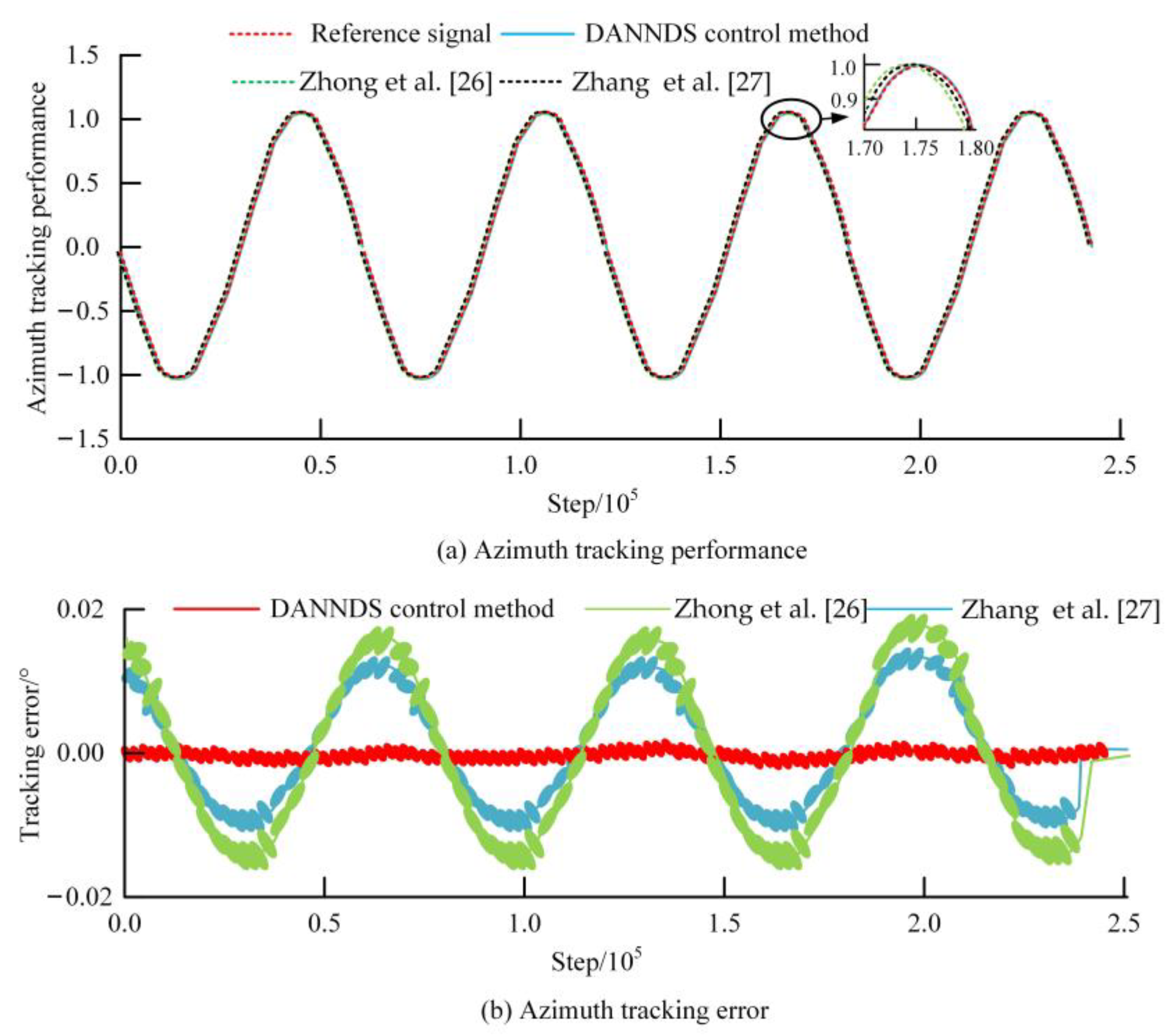
Figure 6 shows the azimuth tracking performance and tracking error results of the three control methods. Figure 6a shows the variation curves of the azimuth tracking performance of the three control methods. As the step size increases, the tracking performance of the three methods shows periodic variation curves, and the DANNDS control method is more in line with the change in the reference signal. The variation curves of the other two control methods have a certain gap with the curve of the reference signal. This indicates that the proposed method can more efficiently track changes in solar light. According to Figure 6b, as the step size increases, the tracking error of the DANNDS control method changes slightly, ranging within [−0.003,0.003]. The tracking error curve of the control method proposed in the literature [26] shows periodic fluctuations with a large amplitude. The control method designed in the literature [27] has the maximum tracking error, with a range of variations within [−0.17,0.017]. In summary, the tracking effect and performance of the DANNDS control method are superior to those of the other two mainstream control methods.
Figure 7 shows the variation curves of the height angle quantization control signals for the two quantization methods, wherein random interference signals were introduced at steps 0.4 × 10⁵ and 1.7 × 10⁵. The variation curves of the two methods exhibit the same periodic variation, with logarithmic quantization within the range of [−20,20] and more frequent fluctuations. The hysteresis quantification method proposed in this study varies with step size within the range of [−8,8], and the fluctuations are smoother. At the two points where the random interference signals were introduced, the proposed hysteresis quantizer can better alleviate the adverse effects caused by the introduction of random interference.
Figure 8 shows the comparison of the azimuth quantization control signals of the two quantization methods. Both quantization methods exhibit similar periodic trends, and the fluctuation range of the logarithmic quantization change curve is [−20,20], with corresponding changes fluctuating more frequently. The fluctuation range for the change curve of the hysteresis quantification method is [−19,19], and the corresponding change fluctuation is relatively flat. To sum up, the proposed hysteresis quantizer can effectively suppress the chattering phenomenon of the controller, and its performance is better than that of the logarithmic quantizer.
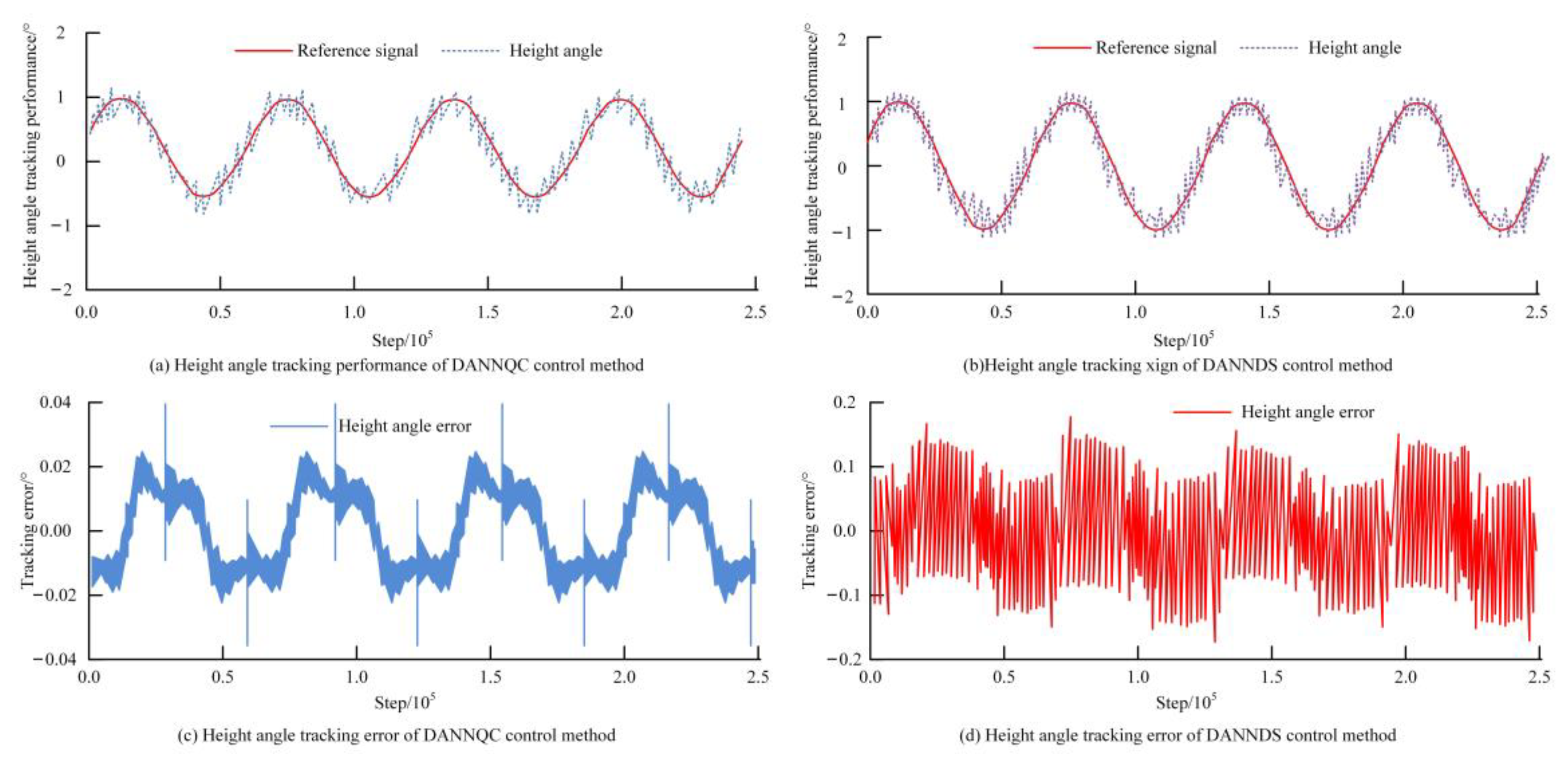
In order to verify the control effect of the DANNQC control method of the photovoltaic power generation servo system, this research carried out experiments on the test platform to obtain the results of the height angle tracking performance and tracking error, as shown in Figure 9. Figure 9a shows the height angle tracking performance change curve of the DANNQC control method, which is very close to the change curve of the reference signal, and the change range is [−1.1,1.1]. Figure 9b shows the height angle tracking performance change curve of the DANNDS control method, which fluctuates more frequently, and the corresponding change range is [−1.2,1.1]. Figure 9c shows the height angle tracking error change curve of the DANNQC control method, which changes periodically on the whole, within the range of [−0.02,0.022]. Figure 9d shows the height angle tracking error change curve of the DANNDS control method, which fluctuates very frequently, and the fluctuation range is [−0.2,0.2].
Figure 10 shows the azimuth tracking performance and tracking error change curve for the DANNQC control method. Figure 10a shows the azimuth tracking performance change curve for the DANNQC control method, which fits well with the reference signal, and the change range is [−1.2,1.1]. Figure 10b shows the azimuth tracking performance change curve for the DANNDS control method, within the range of [−1.2,1.2]. As can be observed in Figure 10c, as the step size increases, the azimuth tracking error for the DANNQC control method presents periodic changes, and the range of these changes is [−0.03,0.03]. Figure 10d shows the azimuth tracking error for the DANNDS control method, which fluctuates frequently and varies in the range of [−1.8,1.8]. In conclusion, the control performance of the DANNQC control method is superior.
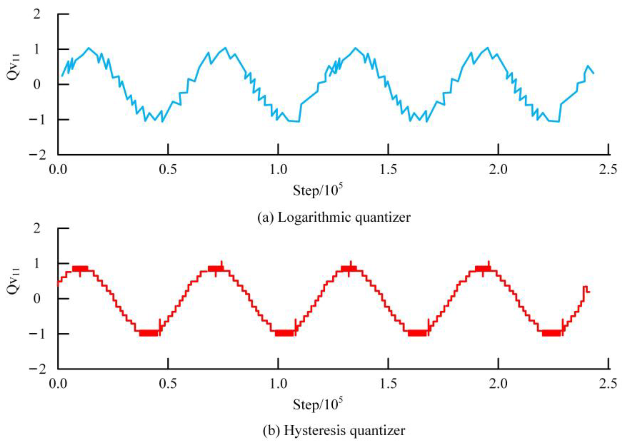
Figure 11 shows the comparison between the hysteresis quantization curve and the logarithmic quantization curve of the output of the photovoltaic power generation servo system based on the DANNQC. Figure 11a shows the quantization effect of the logarithmic quantizer, which fluctuates more frequently. Figure 11b shows the quantization effect of the hysteresis quantizer, which fluctuates more regularly and has a small fluctuation. To sum up, the influence of the quantization effect on the control performance of the photovoltaic power generation servo system is based on the DANNQC.

5. Conclusions

As the energy problem has become increasingly serious in recent years, to achieve the sustainable use of resources, countries around the world are committed to researching new energy. Photovoltaic power generation is an important direction in the development of new energy, but it has shortcomings such as low power generation efficiency. To improve the efficiency of photovoltaic power generation, a DANNDS controller was proposed, and then a DANNQC photovoltaic power generation servo system was constructed based on the DANNDS controller. The experimental results demonstrate the MTE, RMSTE, and 2NTE scores of the height angle servo motor of the DANNDS control method, which were 0.0026, 7.0279 × 10⁻⁴, and 0.3552, respectively. The scores for the various indicators of the azimuth servo motor were 0.3552, 0.0028, 8.9237 × 10⁻⁴, and 0.4511, respectively, which are lower than the scores of the other two mainstream control methods. In the height angle tracking error variation curves, the variation range for the DANNQC control method was [−0.02,0.022]. The fluctuation range for the DANNDS control method was [−0.2,0.2]. In the azimuth tracking error variation curves, the variation range for the DANNQC control method was [−0.03,0.03]. The range for the DANNDS control method was [−1.8,1.8]. To sum up, the DANNDS controller proposed in this study has good steady-state performance, and the photovoltaic power generation servo system based on the DANNQC has better control performance. However, there are still shortcomings in this research. The control schemes proposed in this study are all based on a single photovoltaic power generation servo system. In future research, the collaborative control of multiple photovoltaic power generation servo systems can be studied.

Author Contributions

Conceptualization, original draft preparation, X.X. and W.X. (Wenhua Xu); methodology, writing—original draft preparation, D.N. and K.W.; software, data curation, S.C.; validation, formal analysis, Y.N. and X.F.; investigation, resources, W.X. (Wan Xu). All authors have read and agreed to the published version of the manuscript.

Funding

This research received no external funding.

Data Availability Statement

The datasets used and/or analyzed during the current study are available from the corresponding author on reasonable request.

Conflicts of Interest

The authors declare no conflict of interest.

References

  1. Mathi, R.; Jayalalitha, S. Influence of renewable energy sources on the scheduling on thermal power stations and its optimization for CO2 reduction. Comput. Intell. 2022, 38, 903–920. [Google Scholar] [CrossRef]
  2. Sun, Q.; Yu, L.; Zheng, Y.; Tao, J.; Sun, H.; Dehmer, M.; Chen, Z. Trajectory tracking control of powered parafoil system based on sliding mode control in a complex environment. Aerosp. Sci. Technol. 2022, 122, 107406. [Google Scholar] [CrossRef]
  3. Celikel, R.; Yilmaz, M.; Gundogdu, A. A voltage scanning-based MPPT method for PV power systems under complex partial shading conditions. Renew. Energy 2022, 184, 361–373. [Google Scholar] [CrossRef]
  4. Khaki, B.; Kili, H.; Yilmaz, M.; Shafie, M.; Catalo JP, S. Active Fault Tolerant Control of Grid-Connected DER: Diagnosis and Reconfiguration. In Proceedings of the IECON 2019—45th Annual Conference of the IEEE Industrial Electronics Society, Lisbon, Portugal, 14–17 October 2019; IEEE: New York, NY, USA, 2019. [Google Scholar]
  5. Tong, M.; Lin, W.; Huo, X.; Jin, Z.; Miao, C. A model-free fuzzy adaptive trajectory tracking control algorithm based on dynamic surface control. Int. J. Adv. Robot. Syst. 2020, 17, 578–587. [Google Scholar] [CrossRef]
  6. Wang, M.; Wang, Z.; Chen, Y.; Sheng, W. Observer-based fuzzy output-feedback control for discrete-time strict-feedback nonlinear systems with stochastic noises. IEEE Trans. Cybern. 2020, 50, 3766–3777. [Google Scholar] [CrossRef] [PubMed]
  7. Galtung, S.T.; Raynaud, X. A semi-discrete scheme derived from variational principles for global conservative solutions of a Camassa-Holm system. Nonlinearity 2021, 34, 2220–2274. [Google Scholar] [CrossRef]
  8. Lt, A.; Yh, A.; Shuang, L.B.; Ss, A.; Jd, C.; Hz, D. Application of photovoltaic power generation in rail transit power supply system under the background of energy low carbon transformation. Alex. Eng. J. 2021, 60, 5167–5174. [Google Scholar]
  9. Güllü, E.; Demirdelen, T.; Gurdal, Y.; Mert, B.D.; Nazligul, H. Experimental and theoretical study: Design and implementation of a floating photovoltaic system for hydrogen production. Int. J. Energy Res. 2022, 46, 5083–5098. [Google Scholar] [CrossRef]
  10. Panigrahi, P.K.; Mishra, D.P.; Das, B.; Das, S.R.; Salkuti, S.R. Power quality improvement in a photovoltaic based microgrid integrated network using multilevel inverter. Int. J. Emerg. Electr. Power Syst. 2021, 23, 197–209. [Google Scholar]
  11. Mathivanan, V.; Ramabadran, R. Development and control of a photovoltaic fed flywheel energy storage system for power conditioning. ECS Trans. 2022, 107, 5917–5926. [Google Scholar] [CrossRef]
  12. Mei, F.; Gu, J.; Lu, J.; Zhegn, J. Day-ahead nonparametric probabilistic forecasting of photovoltaic power generation based on the LSTM-QRA ensemble model. IEEE Access 2020, 8, 166138–166149. [Google Scholar] [CrossRef]
  13. Liu, H.; Yuan, H.; Liu, Q.; Hou, J.; Zeng, H.; Kwong, S. A hybrid compression framework for color attributes of static 3D Point Clouds. IEEE Trans. Circuits Syst. Video Technol. 2022, 32, 1564–1577. [Google Scholar] [CrossRef]
  14. Umer, R.; Touqeer, M.; Omar, A.H.; Ahmadian, A.; Salahshour, S.; Ferrara, M. Selection of solar tracking system using extended TOPSIS technique with interval type-2 pythagorean fuzzy numbers. Optim. Eng. 2021, 22, 2205–2231. [Google Scholar] [CrossRef]
  15. Saeedi, M.; Effatnejad, R. A New Design of Dual-Axis Solar Tracking System with LDR sensors by Using the Wheatstone Bridge Circuit. IEEE Sens. J. 2021, 21, 14915–14922. [Google Scholar] [CrossRef]
  16. Anuraj, A.; Gandhi, R. Solar Tracking System Using Stepper Motor. Int. J. Electron. Eng. Res. 2021, 13, 133–138. [Google Scholar]
  17. Fb, A.; Hfo, B.; Fs, C. Experimental study for the application of different cooling techniques in photovoltaic (PV) panels—ScienceDirect. Energy Convers. Manag. 2020, 212, 112789.1–112789.9. [Google Scholar]
  18. Bashar, H.; Ahmed, M.; Ahmed, G. Design and Practical Implementation of Dual-Axis Solar Tracking System with Smart Monitoring System. Prz. Elektrotechniczny 2020, 1, 153–157. [Google Scholar]
  19. Abir Muntacir, A.; Ariful, A.; Umme, H. Design, construct and Performance Study of Microcontroller Based Self-Powered Dual-Axis Solar Tracking System for Photovoltaic Panel. IOSR J. Electr. Electron. Eng. 2020, 15, 40–47. [Google Scholar]
  20. Faydasicok, O. An improved Lyapunov functional with application to stability of Cohen-Grossberg neural networks of neutral-type with multiple delays. Neural Netw. 2020, 132, 532–539. [Google Scholar] [CrossRef]
  21. Ge, L.; Du, T.; Li, C.; Li, Y.; Yan, J.; Rafiq, M.U. Virtual collection for distributed photovoltaic data: Challenges, methodologies, and applications. Energies 2022, 15, 8783. [Google Scholar] [CrossRef]
  22. Bae, J.S.; Oh, S.K.; Pedrycz, W.; Fu, Z. Design of fuzzy radial basis function neural network classifier based on information data preprocessing for recycling black plastic wastes: Comparative studies of ATR FT-IR and Raman spectroscopy. Appl. Intell. 2019, 49, 929–949. [Google Scholar] [CrossRef]
  23. Zhang, W.; Zheng, Z.; Liu, H. Droop control method to achieve maximum power output of photovoltaic for parallel inverter system. CSEE J. Power Energy Syst. 2022, 8, 1636–1645. [Google Scholar]
  24. Xu, B.; Guo, Y. A novel DVL calibration method based on robust invariant extended Kalman filter. IEEE Trans. Veh. Technol. 2022, 71, 9422–9434. [Google Scholar] [CrossRef]
  25. Kim, J.; Tianshu, X.U.; Tsuneoka, Y.; Tanabe, S.; Morito, N. Empirical study on effective utilization of photovoltaic power generation by precooling and preheating operation in house. J. Environ. Eng. Trans. AIJ 2019, 84, 73–81. [Google Scholar] [CrossRef]
  26. Zhong, C.; Zhou, Y.; Zhang, X.P.; Yan, G. Flexible power-point-tracking-based frequency regulation strategy for PV system. IET Renew. Power Gener. 2020, 14, 1797–1807. [Google Scholar] [CrossRef]
  27. Zhang, X.; Shi, R. Research on adaptive non-singular fast terminal sliding mode control based on variable exponential power reaching law in manipulators. Proc. Inst. Mech. Eng. Part I J. Syst. Control. Eng. 2022, 236, 567–578. [Google Scholar] [CrossRef]
Figure 1. Structure of RBFNN.
Processes 11 01667 g001
Figure 2. Hysteresis quantizer at x ( m ) 0 .
Processes 11 01667 g002
Figure 3. Structure of DANNDS control scheme.
Processes 11 01667 g003
Figure 4. Discrete adaptive dynamic surface control structure scheme based on DANNQC.
Processes 11 01667 g004
Figure 5. Height angle tracking performance and tracking error results of three control methods.
Processes 11 01667 g005
Figure 6. Azimuth tracking performance and tracking error results of three control methods.
Processes 11 01667 g006
Figure 7. Height angle quantization control signals of two quantization methods.
Processes 11 01667 g007
Figure 8. Azimuth quantization control signals of two quantization methods.
Processes 11 01667 g008
Figure 9. Height angle tracking performance and tracking error change curve of DANNDS control method and DANNQC control method.
Processes 11 01667 g009
Figure 10. Azimuth tracking performance and tracking error change curve of DANNDS control method and DANNQC control method.
Processes 11 01667 g010
Figure 11. Comparison of two quantization methods in terms of u 11 .
Processes 11 01667 g011
Table 1. Tracking error results of two control methods.
Error TypeMTERMSTE2NTE
DANNDS control methodG0.00267.0279 × 10−40.3552
F0.00288.9237 × 10−40.4511
Zhong et al. [26]G0.01230.00723.6400
F0.01280.00683.4539
Zhang et al. [27]G0.01370.00693.8241
F0.01390.00623.7967
Disclaimer/Publisher’s Note: The statements, opinions and data contained in all publications are solely those of the individual author(s) and contributor(s) and not of MDPI and/or the editor(s). MDPI and/or the editor(s) disclaim responsibility for any injury to people or property resulting from any ideas, methods, instructions or products referred to in the content.

