Article

Study on Internal Flow Characteristics and Abrasive Wear of Pelton Turbine in Sand Laden Water

1
Key Laboratory of Fluid and Power Machinery, Ministry of Education, Xihua University, Chengdu 610039, China
2
CHN Energy Dadu River Geshizha Hydropower Development Co., Ltd., Ganzi 626300, China
3
College of Water Resources and Civil Engineering, China Agricultural University, Beijing 100083, China
*
Authors to whom correspondence should be addressed.
Processes 2023, 11(5), 1570; https://doi.org/10.3390/pr11051570
Submission received: 30 March 2023 / Revised: 18 May 2023 / Accepted: 19 May 2023 / Published: 21 May 2023
(This article belongs to the Section Chemical Processes and Systems)

Abstract

:
When a Pelton turbine operates in sand laden water, the abrasive wear of its overflow components by high-speed jets is serious. Based on the VOF (volume of fluid) multiphase flow model, the SST (shear stress transfer) k-ω turbulence model, the particle motion Lagrangian model, the generic wear model, and the SIMPLEC (Semi-Implicit Method for Pressure Linked Equations Consistent) algorithm, the liquid–air–solid three-phase flow in the key overflow components of a Pelton turbine were simulated, the abrasive wear was predicted, and the internal sand-water flow characteristics and the abrasive wear of the overflow components were analyzed. The results show that the trailing edge at the root of the runner bucket, the leading face of the bucket near the root, the notch, and the splitter are severely worn. The abrasive wear of the splitter and the notch is more severe than that of the leading face of the bucket. The wear rate from the splitter to the trailing edge increases first and then decreases. The wear pattern of the needle tip is mainly “dotted”, while that of the nozzle opening is “flaky”, and the abrasive wear of the nozzle opening is more severe than that of the needle. The predicted results are consistent with the actual conditions at the site of the power station. This study provides a technical method for the prediction of abrasive wear of the Pelton turbine and a technical basis for the operation and maintenance of the power station.

1. Introduction

The Pelton turbine is the optimal choice for power generation on rivers with ultra-high head in Southwest China. However, the rivers in this region carry sand particles which will flow through the operating turbine units, especially during the flood season. The overflow components of the turbine will be worn and eroded, which will reduce the power generation efficiency and increase the maintenance frequency, resulting in huge economic losses. Characterized by the high velocity jet, the wear and tear of the overflow components of the Pelton turbine will be much more serious, so great importance is attached to the site selection and the abrasive wear resistance design of the Pelton turbine.
The operation of turbines in turbid water, due to the serious soil erosion in recent years, has drawn the attention of scholars to study the abrasive wear of turbine components. Bajracharya et al. [1] predicted that the wear rate for the needle and the buckets is 3.4 mm/year, resulting in a 1.21% reduction in efficiency. Rai et al. [2,3,4,5] scaled down the bucket of a Pelton turbine and conducted experiments with different sand sizes and concentrations, obtained a wear model for the bucket by the multiple regression analysis, and found that the velocity had a greater effect on abrasive wear than other parameters. Leguizamon et al. [6,7] proposed a multiscale model of abrasive wear to predict the wear depth and rate at three impingement angles and performed an error propagation analysis of the comparison between simulation and field data, yielding an uncertainty of ±22%. Based on the experimental data collected for different parameters, Padhy et al. [8,9] developed a correlation for the wear rate and the efficiency loss with the size and concentration of silt particles, jet velocity, and operating hours, and found that the calculated wear rate deviates from the experimental data within 6.7%. On the basis of measurement of material removed by the process of erosion, Din et al. [10] quantified the hydro-abrasive wear of the spear and nozzle as 3.71% and 5%, respectively. Tarodiya et al. [11] found that the wear resistance of the Pelton injector improves by an order of 100 with a coating of WC-CoCr, and the coated surface improves the uniformity in wear distribution.
Some scholars have studied the Pelton turbine model optimization, jet interaction, secondary flow, and wear characteristics of overflow components by numerical simulation. Kim et al. [12] developed a theoretical formula for determining the optimal number of buckets required for achieving the maximum possible efficiency of a Pelton turbine and validated the formula by conducting a performance test on a pico-scale Pelton turbine by using runners with different numbers of buckets. Židonis et al. [13] found that the number, the radial position, and the angular position of buckets were interrelated. Benzon et al. [14] optimized the design of the injector and found that the improved geometry produces a jet profile which induces better overall runner performance, giving a 0.5% increase in total hydraulic efficiency for the Pelton case and 0.7% for the Turgo case. Anagnostopoulos et al. [15] used a stochastic optimizer based on an evolutionary algorithm to numerically optimize the bucket shape. Jeon et al. [16] found that a large friction loss is generated in an injector if the spear is closed too tightly for a low flow rate below the critical value, and the head loss is doubled. Jung et al. [17] found that pressure deviation caused by jet eccentricity and jet velocity imbalance are the main causes of jet diffusion. Nedelcu et al. [18] found that the largest effect on flow variation is the head, followed by the opening and the nozzle diameter. Alimirzazadeh et al. [19] simulated the interaction between two adjacent jets under eight operating conditions based on the finite volume particle method and found that jet perturbations produce load fluctuations and may exacerbate fatigue at speeds below and above the optimum efficiency point. Gupta et al. [20] estimated the efficiency, bucket load, water velocity, and water phase distribution at different rotational speeds. Egusquiza et al. [21] developed a theoretical model to simulate the dynamic behavior of the Pelton turbine from which the deformations and stresses of the runner can be computed. Chongji Zeng et al. [22,23] found, by numerical prediction, that the residual kinetic energy carried by the outflow at non-design heads is the main cause of efficiency loss in Pelton turbines, and that a reduction in the head or the angle between two jets leads to flow interference between adjacent jets. Rossetti et al. [24] analyzed the time-varying effect of water bucket geometry on energy exchange based on a hybrid Euler-Lagrange approach. Han et al. [25,26,27] found that the particles were more concentrated in the inner side of the nozzle after the contraction section, analyzed the vortex structure and secondary flow in the distributor and nozzle, and found that sand particles interfered with the water distribution, thus reducing the total torque and the hydraulic efficiency by about 9%. Xiao Yexiang et al. [28,29] proposed a new algorithm to predict the impact behavior of particles and analyzed the flow and wear characteristics of the water bucket during rotation.
This work combines the numerical simulation with the actual wear of the power station for a comprehensive analysis and with the actual situation to ensure the accuracy of the numerical simulation results. This study was based on the VOF multiphase flow model, the SST k-ω turbulence model, the particle motion Lagrangian model, and the generic wear model [30]. The liquid–air–solid three-phase flow in the whole Pelton turbine was numerically simulated, the abrasive wear of key overflow components was predicted, and then the sand-water flow characteristics and the wear conditions of the overflow components were analyzed.

2. Mathematical Models

2.1. Multiphase Flow Model

The internal flow of a Pelton turbine in sand laden water is actually a liquid–gas–solid three-phase flow. The VOF model can simulate the multiple immiscible fluids by solving a single momentum equation and tracking the volume fraction of each fluid in the region [31]. In each control body, the sum of the volume fractions α of all phases is 1, i.e., Σαi = 1, and:
ρ = α i ρ i
μ = α i u i
t α i ρ i + α i ρ i v i = 0
where α is the volume fraction, ρ is the density, μ is the dynamic viscosity, and the subscript i is the tensor coordinate (indicating the liquid, gas, or solid phase).

2.2. Turbulence Model

The SST k-ω model is an improved version of the standard k-ω model, which combines the advantages of the k-ω and k-ε models to simulate rotating shear flows at high Reynolds numbers and are applicable to the Pelton turbine. The transport equation of the SST k-ω model is as follows:
t ρ k + x i ρ k u i = x j Γ k k x j + G k Y k + S k
t ρ ω + x i ρ ω u i = x j Γ ω ω x j + G ω Y ω + D ω + S ω
where Gk is the turbulent kinetic energy k-generation term, Gω is the ω-generation term Γ k , and Γ ω are effective diffusion terms for k and ω, Yk and Yω are turbulent dissipation terms for k and ω, respectively, Dω is the orthogonal divergence term, Sk and Sω are the user-defined source terms.

2.3. Particle Trajectory Model

The trajectory of discrete-phase particles in multiphase flow were tracked by using a particle motion Lagrangian equation model [32]. The control equation for the discrete-phase particles is as follows:
m p d u p d t = m p u u p τ r + m p g ρ p ρ ρ p + F
F = 3 4 d p C D u V u p V u i u p i + 3 2 d p K B v π t d u i d τ d u p i d τ d τ t τ + 6 π d p K S v u j x i 1 2 u j u p j sgn u j x i + 3 4 C M Ω i × u i u p i + K M d u i d t 1 ρ p x i
where mp is the particle mass, u is the fluid phase velocity, u p is the particle velocity, ρ p ρ is the density difference term between the particle and the fluid, F is an additional force, m p u u p τ r is the drag force, and τ r is the droplet or particle relaxation time calculated by: τ r = ρ p d p 2 18 μ 24 C d Re . Re is the relative Reynolds number, which is defined as: Re = ρ d p u p u μ . m p g ρ p ρ ρ p is the particle buoyancy; CD is the particle drag coefficient, CD = 0.44; dp is the particle size, dp = 0.1 mm; KB is the Basset force coefficient, KB ≈ 6.0; ν is the fluid kinematic viscosity; KS is the Saffman lift coefficient, KS ≈ 1.615; Km is the virtual mass force coefficient, Km ≈ 0.5; CM is the Magnus lift coefficient, CM ≈ 1.0; ωp is the angular velocity of the particle’s own rotation; p is the pressure; g is the acceleration of gravity; sgn is the sign function; and ρ ¯ is a ratio, representing the ratio of the density of sediment particles to the density of water.
The momentum transfer from the continuous phase to the discrete phase is computed in Ansys Fluent by examining the change in momentum of a particle as it passes through each control volume in the Ansys Fluent model. This momentum change is computed as:
F = 18 μ C D R e 24 ρ p d p 2 u p u + F o t h e r m ˙ p t
where m ˙ p is the mass flow rate of the particles, Δt is the time step, Fother is other interaction forces. This momentum exchange appears as a momentum source in the continuous phase momentum balance in any subsequent calculations of the continuous phase flow field.

2.4. Wear Model

When sand laden water flows through the injector, the nozzle and the needle are subjected to abrasive wear, and when the jet impacts the bucket, the bucket surface will also be worn. The generic wear model was used to predict the wear distribution and wear rate of the overflow components [33]; the expression is as follows:
R e = p = 1 N P m ˙ p c d p f α 1 w b w A f
where Re is the wear rate, NP is the total number of particles, m ˙ p is the particle mass flow rate, c(dp) is the particle size function, f(α1) is the angle function (α1 is the angle at which the particles impact the wall), b(w) is a function of the relative velocity of the particles (w is the relative velocity of the particles to the wall), and Af is the wall area. The wear rate in Ansys Fluent is shown in units of material removed/(area—time), i.e., mass flux. This study calculates the wear rate based on length/time (mm/s) by dividing the wear rate by the density of the wall material.

3. Computational Geometry Physical Model and Boundary Conditions

3.1. 3D Geometric Physical Modeling of Overflow Components

The Jiniu Hydropower Station on the main stream of the Geshizha River in Danba County, Sichuan Province, China, was taken as the research object. A computational geometric model of the turbine overflow components was established based on the turbine design and other data. The basic design parameters of the turbine are listed in Table 1, in which the metal materials of the overflow components are as follows: the nozzle and needle material is made of 00Cr13Ni5Mo and the runner material is made of X3CrNi13-4. The solid structure of the runner is shown in Figure 1.
The three-dimensional geometric model of the computational domain of the turbine is shown in Figure 2. It mainly consists of the following four parts: ① the rotating domain of the bucket, ② the annular stationary domain outside the rotating domain, ③ the jet domain at the nozzle outlet, and ④ the injector consisting of the nozzle and needle.

3.2. Geometric Model Meshing

The Pelton turbine has a complex structure, so a polyhedral unstructured grid is used to mesh the rotor while a structured grid is used for the injector. The grid division of bucket and injector is shown in Figure 3. Since the number of grids has a large impact on the results of numerical simulation, the grid of the whole flow field was verified to be irrelevant, and the results are listed in Table 2. With the increasing of the number of grids, the predicted efficiency gradually approaches the design efficiency. Considering the computational resources and the accuracy of numerical simulation, Option 2 was chosen.

3.3. Computational Boundary Conditions

Ansys Fluent was used for this numerical simulation. The inlet boundary was adopted as the velocity inlet with a flow velocity rate of 7.51 m/s, while the outlet boundary was set as pressure outlet with a pressure of 0 Pa. The rotating domain was connected with the stationary domain by a cross interface. The fixed wall surface was adopted as the no-slip boundary condition, and the standard wall surface function was used to simulate the flow in the near-wall surface region. The discrete phase adopts bidirectional coupling, considering the interaction between the discrete phase and the continuous phase, and the effect of turbulence on the particles is also taken into account to turn on the discrete random walk model. Additionally, the discrete phase particles were simplified as spherical particles, which were injected perpendicular to the inlet surface, the incidence velocity was kept consistent with the water flow velocity, and the contact mode with the wall surface were set as rebound. The normal and tangential bounce coefficients of the particles on the wall are defined as polynomial functions of the impact angle of the particles. The normal bounce coefficient εN and the tangential bounce coefficient εT are defined as follows:
ε N = 0.993 0.0307 α 1 + 4.75 × 10 4 α 1 2 2.61 × 10 6 α 1 3
ε T = 0.998 0.029 α 1 + 6.43 × 10 4 α 1 2 3.56 × 10 6 α 1 3

4. Numerical Calculation and Results Analysis

The SIMPLEC algorithm was used for calculation, the time step was set as 1.11 × 10⁻⁴ s, and each time step was iterated 20 times. Water and air were considered continuous phases and discrete-phase particles were added for the liquid–air–solid three-phase flow calculation. The discrete phases were coupled in both directions. Considering the interaction between the discrete phases and the continuous phases, the trajectory was calculated once every 10 steps of the continuous-phase iteration. The hydrological sand parameters of Jiniu Hydropower Station are listed in Table 3.

4.1. Flow Characteristics in the Bucket

Since the torque of each bucket is cyclic, a single bucket was studied and the variation of the torque with time was monitored during the calculation, and the torque–time curve for a time period was extracted, as shown in Figure 4. Three time points t1 (torque rising phase), t2 (high torque phase), and t3 (torque dropping phase) were selected within this period, and the corresponding water phase distribution is shown in Figure 4 (from bottom to top for bucket 1#, bucket 2#, and bucket 3#), and the flow characteristics of bucket 2# at these three time points were analyzed.

4.1.1. Velocity Distribution

The calculated velocity and streamline distribution on the leading face of the bucket are shown in Figure 5. At the time t1, the jet only strikes the head of the splitter, where the flow velocity is large and the direction of the streamline is at an acute angle with the splitter; meanwhile, the flow velocity is smaller at the trailing edge, and the streamlines on the side of the splitter and near the trailing edge on that side are gathered in one direction. At the time t2, part of the jet strikes vertically at the base circle of the bucket, where the direction of the streamline is at a right angle with the splitter. At this time, the velocity at the splitter is the largest and is decreasing along the streamlines to both sides of the trailing edge, and the water flow is fully extended in the direction of the trailing edge. At the time t3, there are still some fluids in the bucket, the velocity decreases along the splitter to both sides of the trailing edge, reaches a minimum value at the leading face of the bucket near the trailing edge, and the streamlines on a single side converge in one direction.

4.1.2. Pressure Distribution on Bucket Leading Face

The calculated pressure distribution on the bucket leading face is shown in Figure 6. At the time t1, the jet is partially intercepted by the head of the splitter of the 2# bucket, resulting in a local high-pressure area, and there is also a small part of the pressure area generated by the jet on both sides of the splitter. As more and more of the jets are intercepted by the #2 bucket, the torque of the #2 bucket continues to rise. At the time t2, the jet is partially intercepted by the 3# bucket, and part of the jet strikes the base circle of the 2# bucket. At this time, the torque of the 2# bucket reaches the maximum value in this cycle, the high-pressure area is symmetrically distributed on both sides of the splitter, the high-pressure area at the bottom of the bucket is shifted toward the root of the bucket, and the pressure value gradually decreases from the bottom of the bucket to the splitter. At the time t3, there is no more jet striking the 2# bucket, the torque drops rapidly, the water film on the leading face of the bucket is extended, and the high-pressure area moves towards the trailing edge.

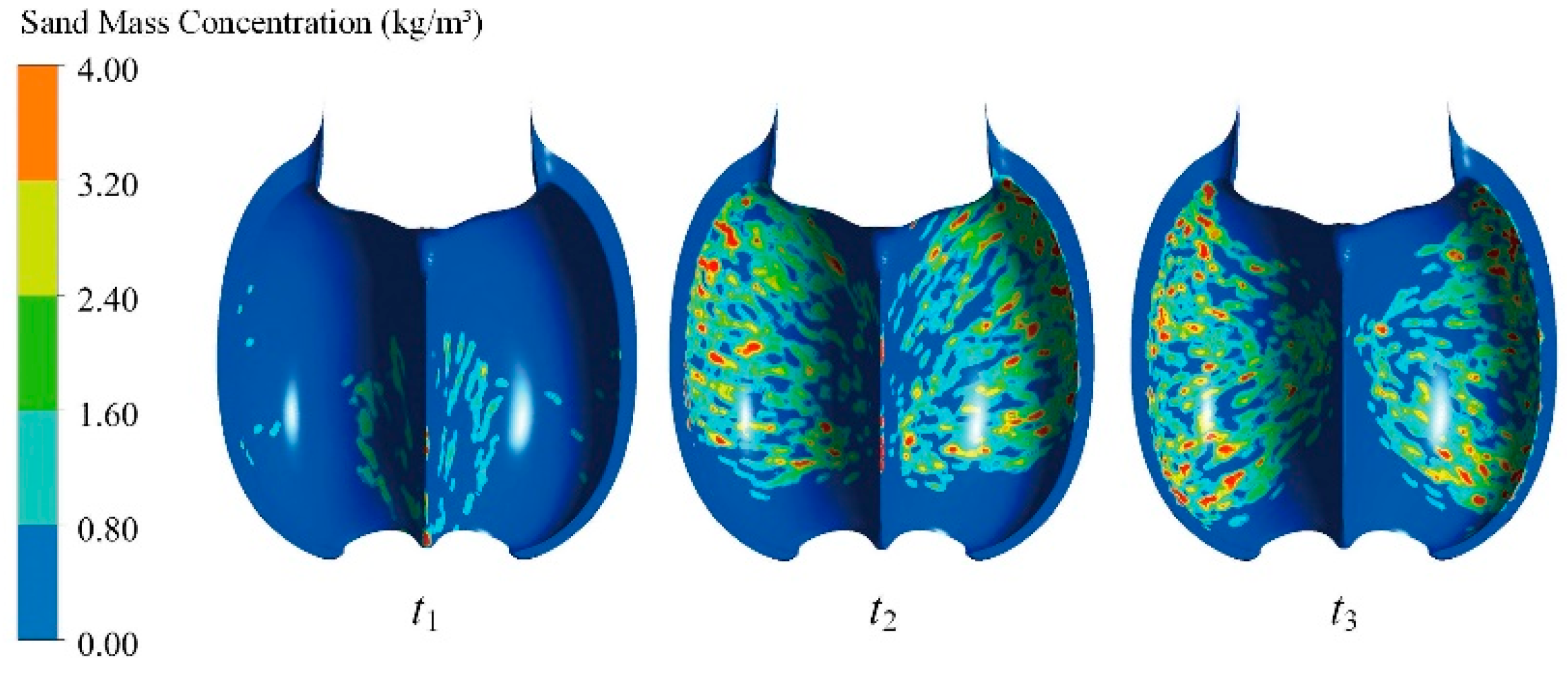
4.1.3. Local Sand Concentration Distribution

The sand concentration distributions on the leading face of the bucket at t1, t2, and t3 were analyzed, as shown in Figure 7. At the time t1, the sand concentration at the head of the splitter is high. At the time t2, the sand concentration at the middle of the splitter is high, the sand distribution on both sides of the splitter is wide, and the sand is distributed symmetrically on both sides of the splitter. At the time t3, there is no obvious sand distribution at the splitter and the sand distribution range from the splitter to the trailing edge gradually expands. As shown in Figure 8, the sand particles carried in the sand laden water are evenly distributed along the splitter to both sides of the trailing edge, while the sand content and concentration on the surface of the 2# bucket are larger than those of the 1# bucket and 3# bucket. Although the 3# bucket intercepts part of the jet stream, the jet stream has not hit the base circle so the sand concentration at the splitter of the 3# bucket is low and the sand particles are mainly distributed on both sides near the splitter. At the same time, sand particles are still gathered at the bottom of the 1# bucket and the trailing edge because the fluid from the previous jet has not been completely discharged, and the closer to the leading face, the higher the sand concentration will be.

4.2. Internal Flow Characteristics of the Injector

The injector completely converts the pressure energy into kinetic energy through the nozzle. Before striking the buckets, the jet is in contact with the air. A thin layer of air–water interface will be formed in the jet domain, the stationary domain, and the rotating domain. The water-air volume fraction distribution in the whole flow field is shown in Figure 9 (the figure shows the top view of the whole flow field), with red as the water phase and blue as the gas phase.

4.2.1. Velocity Distribution

A single nozzle was selected to study the velocity distributions of water and sand particles on its horizontal axis. It can be seen from the water velocity cloud in Figure 10a that the flow velocity increases rapidly near the nozzle, and a low velocity zone is formed at the tip of the needle, which is known as the “velocity loss” phenomenon caused by the continuous development of the boundary layer on the needle surface. This phenomenon also affects the velocity distribution in the free jet zone, i.e., the velocity in the center of the jet is relatively low, but it is gradually weakening along the flow direction, and the velocity uniformity of the jet is improved in the region away from the tip of the needle. The velocity distribution of sand particles in the injector is shown in Figure 10b. The velocity of sand particles is maintained at about 95 m/s after being ejected from the nozzle outlet, while the velocity of particles in the center line of the jet is significantly lower.
To analyze the movement of sand and water within different overflow components, the injector is divided into 6 planes along the flow direction, as shown in Figure 11. The velocity clouds of sand particles at 6 cross-sections are shown in Figure 12. It can be seen from S1 to S3 cross-sections in Figure 12 that the velocity of the sand particles is small near the wall, and the velocity of the sand laden water increases as the overflow area decreases. When the sand particles flow through the nozzle outlet, the velocity increases rapidly; in S4 to S6 cross-sections, the injection velocity reaches the maximum and jet area expansion occurs. The phenomenon of “velocity loss” appears in the center of S4 cross-section due to its close distance from the needle tip.

4.2.2. Pressure Distribution

The Pelton turbine injector, as the main structure of water flow energy conversion, coverts the high-pressure water flow into a high-speed jet, which strikes the buckets mounted on the runner, which in turn rotates the runner of the turbine. The pressure cloud in the injector is shown in Figure 13. It can be seen that the pressure at the inlet of the injector is the largest. As the sand laden water flows to the nozzle outlet, the pressure decreases rapidly and forms an annular jet at the interface between the needle and the nozzle. The pressure gradient of the jet changes significantly. However, after the jet breaks away from the nozzle opening, the jet suddenly starts to expand, the pressure gradient is no longer changing uniformly, and a local high-pressure area appears at the tip of the needle.

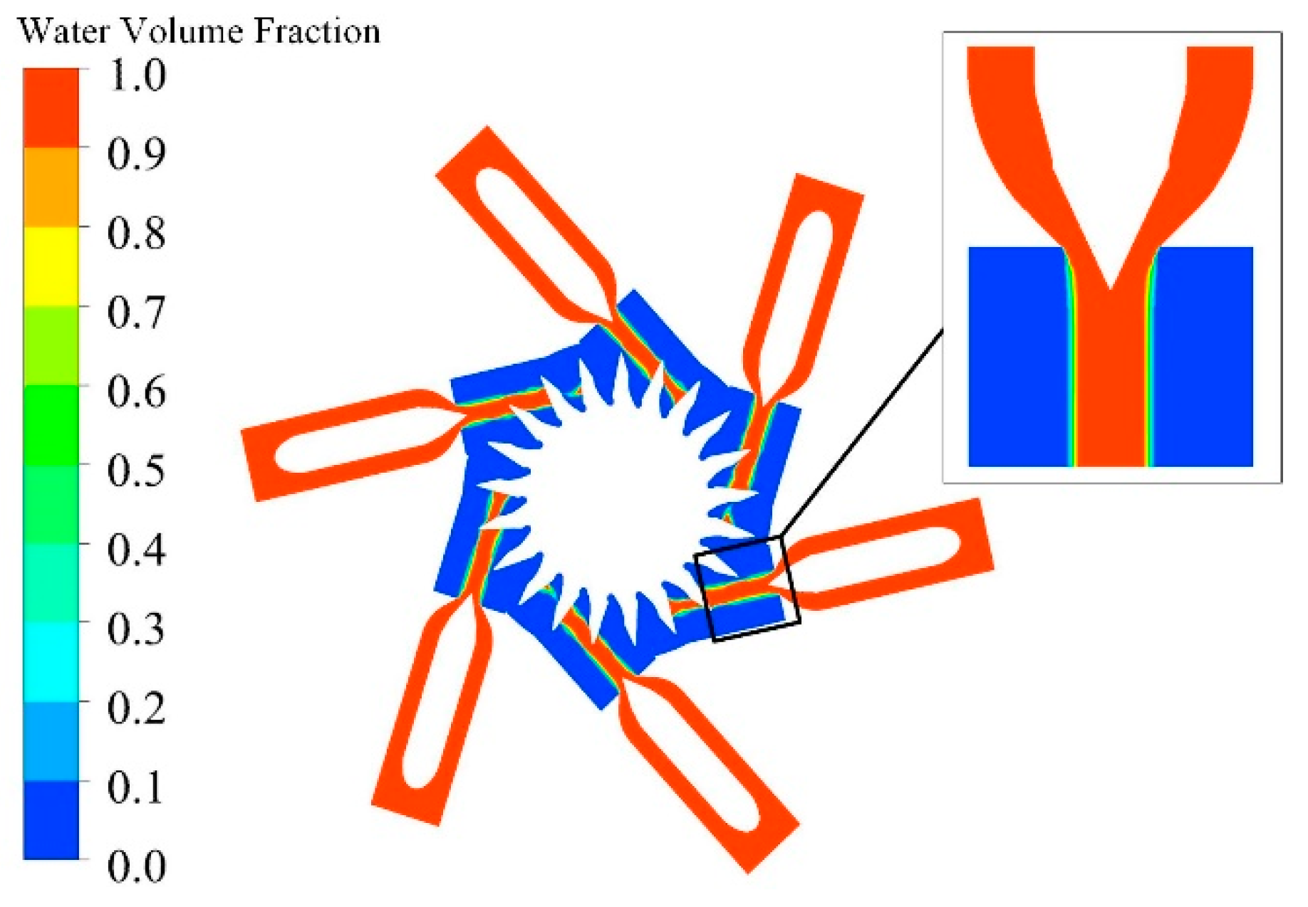
4.2.3. Local Sand Concentration Distribution

The distribution of sand mass concentration inside the injector is shown in Figure 14. The distribution of sand concentration is streamlined at the middle of the needle and on the deflector. Sand particles are mostly distributed at the middle of the needle, less at the tail of the needle. By zooming in on the tail of the needle, it can be seen that most sand particles are gathered at the transition section at the tail of the needle. In addition, there is a local high concentration area at the head of the needle and the head of the deflector, where these sand particles will impact and wear the injector. The distribution of sand mass concentration of a single nozzle is shown in Figure 15. Sand particles with the flow is better—the overall distribution of sand particles in the nozzle is more uniform, particles will scour the wall surface of the spray needle and the nozzle with water flow. Near the tip of the needle, as the sand particles do centrifugal motion relative to the needle, the sand concentration is low near the wall of the needle tip. In Section 4.2.1, it is mentioned that there is a low velocity zone in the center of the jet. From Figure 15, it can also be found that the sand concentration distribution in the low velocity zone is relatively low.

4.3. Abrasive Wear of Runner Bucket

4.3.1. Wear Distribution

The bucket will be severely worn by the striking of the high-speed jet. The wear rate cloud of the bucket leading face is shown in Figure 16. It can be seen that the parts subjected to severe wear are the trailing edge near the root of the bucket, the leading face of the bucket near the root, and the notch and the splitter.
To study the relationship between the wear rate and the relative wear position, the splitter is used as the center (i.e., point 0 of the abscissa), −1~0 represents the chord length of the left half section, and 0~1 represents the chord length of the right half section. The abscissa is defined as the relative position of this point on the section of the base circle (the schematic diagram of the base circle transversal is shown in Figure 17) and the relationship curve is drawn, as shown in Figure 18. It can be seen that the wear at the splitter is the most severe. The wear distribution on both sides of the splitter is symmetrical, and the wear rate in general has a tendency to rise first and fall later, with a slight change in the maximum value. There is certain wear at the trailing edge.

4.3.2. Wear Estimation and Actual Measurement

Jiniu Hydropower Station is the last stage of the “one-reservoir-and-four-stage” hydropower development program on Geshizha River, which is a low-gate diversion type power station. The reservoir can regulate on a daily basis. The power station is installed with two turbine units, and they will be shut down for sand flushing when the power station is the least required in the power system. When the average daily flow rate into the reservoir is greater than 190 m3/s, the power station will also be shut down to avoid the peak flow and the gates will be fully opened for sand flushing. During the flood season, when the flow rate is not large, but the sand content reaches to a certain amount, the power station will also be shut down for sand flushing to avoid abrasive wear of the turbine. According to the hydrological sand information and operation of the power station for many years, it is known that the minerals with the Mohs hardness greater than 5 among the sand particles of the Geshizha River are quartz, feldspar, and green curtain stone, and their contents account for 81.5%. The power station generally operates for 15 days each year when the average maximum sand content is 0.212 kg/m3. After seven years of operation, the abrasive wear of the turbine buckets was tested on site. This study predicted the abrasive wear of the turbine bucket based on the hydrological sand information and the operation data during these seven years. The predicted and measured results are listed in Table 4.
From the predicted data in Table 4, it can be seen that the wear of the splitter and the notch is more severe than that of the bucket leading face, the wear of the splitter is more severe than that of the notch, and the wear of the bucket leading face near the root is also severe.
The abrasive wear of the Pelton turbines in Jiniu Hydropower Station after seven years of operation was measured and photographed on site, and the results also show that the notch and the splitter are the parts with severe wear, as in the oval circle shown in Figure 19. The predicted results of the wear distribution on the bucket leading face are consistent with the measured results. Meanwhile, some “honeycomb structure” abrasion pits are also found on the surface of the bucket, which should be the result of the combined effect of wear and cavitation.
From the data in Table 4, it can also be seen that the predicted wear results of the turbine bucket are larger than the measured results by 6%. It is believed that this deviation is related to the data accuracy of the hydrological sand information and operating conditions obtained by the power station, as well as the accuracy of the wear model selected for the calculation. However, the deviation of abrasive wear prediction is within the permissible range of the project, and the calculated results can reflect the abrasive wear of the turbine bucket.

4.4. Abrasive Wear of the Injector

4.4.1. Wear Distribution

The calculated wear cloud of the needle is shown in Figure 20. It can be seen that the wear of the tail of the needle and the tail of the deflector is obvious, and the maximum wear rate reaches 1.29 × 10⁻⁷ mm/s. Along the flow direction, the wear of the straight rod section of the needle gradually weakens, which is caused by the even injection of sand particles from the inlet. The section near the inlet of the needle rod is worn by the impact of sand particles. With the development of flow, sand particles on the middle of the needle caused by weak wear, when the particles flow to the needle transition area due to the sudden narrowing of the overflow area, increase the particle flow rate; this section experiences more serious wear. It can also be seen that in the needle tip section, due to the positive curvature shape of the needle tip, the water flow and sand particles movement are centrifugal relative to the needle head, and the wear pattern of the needle tip is mainly “dotted” and “flaky”.
The impact wear of the sand particles and the nozzle mainly occurs at the nozzle outlet. The wear cloud of the nozzle opening is shown in Figure 21. It can be seen that the wear pattern of the nozzle is mainly “flaky”. The distribution of wear is uniform along the nozzle opening. The maximum wear rates of the needle and the nozzle opening reach 1.29 × 10⁻⁷ mm/s and 8.52 × 10⁻⁷ mm/s, respectively, and the wear of the nozzle opening is more severe than that of the needle.

4.4.2. Wear Amount Prediction

According to the abrasive wear rate of the needle and nozzle opening, the wear amounts were estimated after seven years of operation, as listed in Table 5. The needle was replaced twice and the nozzle opening was replaced four times during these seven years.

5. Conclusions

The VOF multiphase flow model, the SST k-ω turbulence model, the particle motion Lagrangian model, and the SIMPLEC algorithm are used to numerically simulate the liquid–air–solid three-phase flow inside a Pelton turbine, and the generic model is used to predict the wear distribution on key overflow components of the turbine. The main conclusions are as follows:
(1)
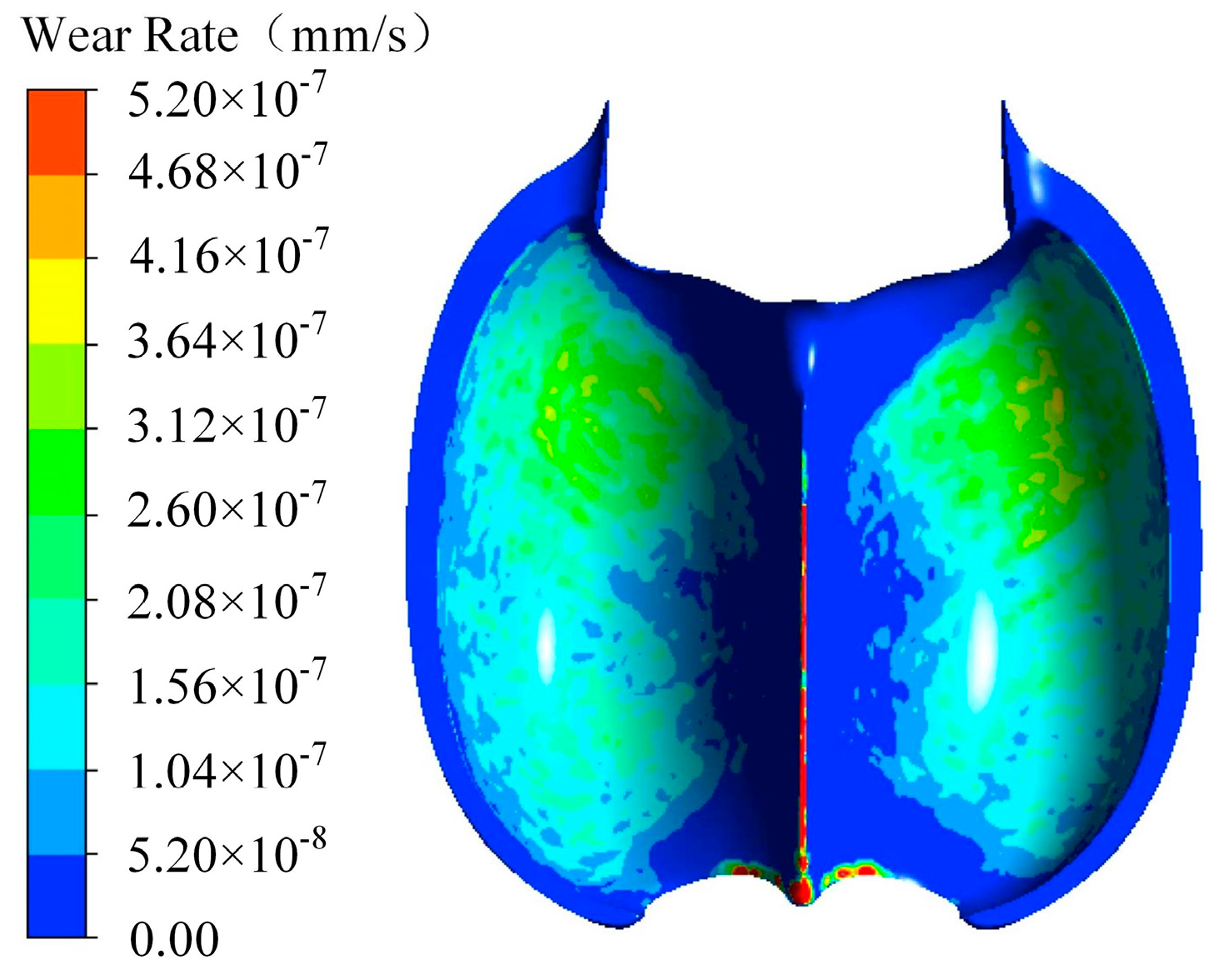
The water trailing edge at the root of the turbine bucket is susceptible to abrasive wear, while the leading face of the bucket near the root, the notch, and the splitter are severely worn. The wear rate from the splitter to the trailing edge increases first and then decreases. The maximum wear rates of the leading face, the notch, and the splitter are 4.19 × 10⁻⁷ mm/s, 5.08 × 10⁻⁷ mm/s, and 5.20 × 10⁻⁷ mm/s, respectively. The wear of the splitter and the notch is more severe than that of the leading face.
(2)
The wear pattern of the needle tip is mainly “dotted” and “flaky”, the wear of the nozzle along the opening is uniformly distributed, and the wear pattern is “flaky”. The maximum wear rates of the needle and the nozzle opening reach 1.29 × 10⁻⁷ mm/s and 8.52 × 10⁻⁷ mm/s, respectively, and the wear of the nozzle opening is more severe than that of the needle.
(3)
The predicted results of turbine bucket wear are consistent with the results measured on site, and the deviation is only about 6%, which indicates that the prediction method is feasible.
(4)
Although the water quality of the Geshizha River is generally good, there is only a brief period of high sand content during heavy rainfall, and attention is paid to avoid the turbine operating during the sand-peak period. This study still finds that the turbine is severely worn, so anti-abrasive wear design and sand-peak avoidance operations are quite important for Pelton turbines. This study provides a technical method and basis for the wear prediction of Pelton turbines and their operation and maintenance.

Author Contributions

Y.H., X.L. and Z.Y. proposed the simulation method. Y.H., H.D., M.Q. and J.L. completed the numerical simulations. Y.H., J.P., X.L. and F.D. analyzed the data and wrote the paper. J.P. and X.L. revised and reviewed the paper. F.D. and Q.Q. provided some data support for the study. All authors have read and agreed to the published version of the manuscript.

Funding

This research was funded by the National Key Research and Development Program of China (approval No. 2018YFB0905200), and the Hydropower Energy Innovation Capacity Construction Project in Sichuan Province, China (approval No. 2022-510124-04-01-622476).

Data Availability Statement

Not applicable.

Conflicts of Interest

The authors declare no conflict of interest.

References

  1. Bajracharya, T.R.; Acharya, B.; Joshi, C.B.; Saini, R.; Dahlhaug, O.G. Sand erosion of Pelton turbine nozzles and buckets: A case study of Chilime Hydropower Plant. Wear 2008, 264, 177–184. [Google Scholar] [CrossRef]
  2. Rai, A.K.; Kumar, A.; Staubli, T.; Yexiang, X. Interpretation and application of the hydro-abrasive erosion model from IEC 62364 (2013) for Pelton turbines. Renew. Energy 2020, 160, 396–408. [Google Scholar] [CrossRef]
  3. Rai, A.K.; Kumar, A.; Staubli, T. Hydro-abrasive erosion in Pelton buckets: Classification and field study. Wear 2017, 392, 8–20. [Google Scholar] [CrossRef]
  4. Rai, A.K.; Kumar, A.; Staubli, T. Analytical modelling and mechanism of hydro-abrasive erosion in Pelton buckets. Wear 2019, 436–437, 203003. [Google Scholar] [CrossRef]
  5. Rai, A.K.; Kumar, A.; Staubli, T. Effect of concentration and size of sediments on hydro-abrasive erosion of Pelton turbine. Renew. Energy 2020, 145, 893–902. [Google Scholar] [CrossRef]
  6. Leguizamón, S.; Jahanbakhsh, E.; Maertens, A.; Alimirzazadeh, S.; Avellan, F. A multiscale model for sediment impact erosion simulation using the finite volume particle method. Wear 2017, 392, 202–212. [Google Scholar] [CrossRef]
  7. Leguizamón, S.; Alimirzazadeh, S.; Jahanbakhsh, E.; Avellan, F. Multiscale simulation of erosive wear in a prototype-scale Pelton runner. Renew. Energy 2020, 151, 204–215. [Google Scholar] [CrossRef]
  8. Padhy, M.K.; Saini, R.P. Effect of size and concentration of silt particles on erosion of Pelton turbine buckets. Energy 2009, 34, 1477–1483. [Google Scholar] [CrossRef]
  9. Padhy, M.K.; Saini, R.P. Study of silt erosion on performance of a Pelton turbine. Energy 2011, 36, 141–147. [Google Scholar] [CrossRef]
  10. Din, M.Z.U.; Harmain, G.A. Assessment of erosive wear of Pelton turbine injector: Nozzle and spear combination–A study of Chenani hydro-power plant. Eng. Fail. Anal. 2020, 116, 104695. [Google Scholar] [CrossRef]
  11. Tarodiya, R.; Khullar, S.; Levy, A. Assessment of erosive wear performance of Pelton turbine injectors using CFD-DEM simulations. Powder Technol. 2022, 408, 117763. [Google Scholar] [CrossRef]
  12. Kim, J.W.; Jo, I.C.; Park, J.H.; Shin, Y.; Chung, J.T. Theoretical method of selecting number of buckets for the design and verification of a Pelton turbine. J. Hydraul. Res. 2017, 55, 695–705. [Google Scholar] [CrossRef]
  13. Židonis, A.; Aggidis, G.A. Pelton turbine: Identifying the optimum number of buckets using CFD. J. Hydrodyn. Ser. B 2016, 28, 75–83. [Google Scholar] [CrossRef]
  14. Benzon, D.; Židonis, A.; Panagiotopoulos, A.; Aggidis, G.A.; Anagnostopoulos, J.S.; Papantonis, D.E. Numerical investigation of the spear valve configuration on the performance of Pelton and Turgo turbine injectors and runners. J. Fluids Eng. 2015, 137, 111201. [Google Scholar] [CrossRef]
  15. Anagnostopoulos, J.S.; Papantonis, D.E. A fast Lagrangian simulation method for flow analysis and runner design in Pelton turbines. J. Hydrodyn. 2012, 24, 930–941. [Google Scholar] [CrossRef]
  16. Jeon, H.; Park, J.H.; Shin, Y.; Choi, M. Friction loss and energy recovery of a Pelton turbine for different spear positions. Renew. Energy 2018, 123, 273–280. [Google Scholar] [CrossRef]
  17. Jung, I.H.; Kim, Y.S.; Shin, D.H.; Chung, J.T.; Shin, Y. Influence of spear needle eccentricity on jet quality in micro Pelton turbine for power generation. Energy 2019, 175, 58–65. [Google Scholar] [CrossRef]
  18. Nedelcu, D.; Cojocaru, V.; Avasiloaie, R.C. Numerical investigation of nozzle jet flow in a pelton microturbine. Machines 2021, 9, 158. [Google Scholar] [CrossRef]
  19. Alimirzazadeh, S.; Kumashiro, T.; Leguizamón, S.; Jahanbakhsh, E.; Maertens, A.; Vessaz, C.; Tani, K.; Avellan, F. GPU-accelerated numerical analysis of jet interference in a six-jet Pelton turbine using Finite Volume Particle Method. Renew. Energy 2020, 148, 234–246. [Google Scholar] [CrossRef]
  20. Gupta, V.; Prasad, V.; Khare, R. Numerical simulation of six jet Pelton turbine model. Energy 2016, 104, 24–32. [Google Scholar] [CrossRef]
  21. Egusquiza, M.; Egusquiza, E.; Valero, C.; Presas, A.; Valentín, D.; Bossio, M. Advanced condition monitoring of Pelton turbines. Measurement 2018, 119, 46–55. [Google Scholar] [CrossRef]
  22. Zeng, C.; Xiao, Y.; Wang, Z.; Zhang, J.; Luo, Y. Numerical analysis of a Pelton bucket free surface sheet flow and dynamic performance affected by operating head. Proc. Inst. Mech. Eng. Part A J. Power Energy 2017, 231, 182–196. [Google Scholar] [CrossRef]
  23. Zeng, C.; Xiao, Y.; Luo, Y.; Zhang, J.; Wang, Z.; Fan, H.; Ahn, S.-H. Hydraulic performance prediction of a prototype four-nozzle Pelton turbine by entire flow path simulation. Renew. Energy 2018, 125, 270–282. [Google Scholar] [CrossRef]
  24. Rossetti, A.; Pavesi, G.; Cavazzini, G.; Santolin, A.; Ardizzon, G. Influence of the bucket geometry on the Pelton performance. Proc. Inst. Mech. Eng. Part A J. Power Energy 2014, 228, 33–45. [Google Scholar] [CrossRef]
  25. Han, L.; Wang, Y.; Zhang, G.F.; Wei, X. The particle induced energy loss mechanism of Pelton turbine. Renew. Energy 2021, 173, 237–248. [Google Scholar] [CrossRef]
  26. Han, L.; Zhang, G.F.; Wang, Y.; Wei, X. Investigation of erosion influence in distribution system and nozzle structure of pelton turbine. Renew. Energy 2021, 178, 1119–1128. [Google Scholar] [CrossRef]
  27. Han, L.; Duan, X.L.; Gong, R.Z.; Zhang, G.; Wang, H.; Wei, X. Physic of secondary flow phenomenon in distributor and bifurcation pipe of Pelton turbine. Renew. Energy 2019, 131, 159–167. [Google Scholar] [CrossRef]
  28. Xiao, Y.; Guo, B.; Zhang, J.; Liang, Q.; Liu, J. Numerical Analysis of the Three-phase Flow and Sand Abrasion of a Pelton turbine. Hydropower Pumped Storage 2021, 7, 4–10. [Google Scholar]
  29. Xiao, Y.; Guo, B.; Rai, A.K.; Liu, J.; Liang, Q.; Zhang, J. Analysis of hydro-abrasive erosion in Pelton buckets using a Eulerian-Lagrangian approach. Renew. Energy 2022, 197, 472–485. [Google Scholar] [CrossRef]
  30. Guo, B.; Xiao, Y.; Rai, A.K.; Liang, Q.; Liu, J. Analysis of the air-water-sediment flow behavior in Pelton buckets using a Eulerian-Lagrangian approach. Energy 2021, 218, 119522. [Google Scholar] [CrossRef]
  31. Pang, J.; Liu, H.; Liu, X.; Ren, M.; Zhang, P.; Yu, Z. Analysis on the escape phenomenon of oil mist from turbine lower guide bearing based on VOF model. Adv. Mech. Eng. 2021, 13, 16878140211060929. [Google Scholar] [CrossRef]
  32. Liu, X.; Cheng, L. Lagrangian model on the turbulent motion of small solid particle in turbulent boundary layer flows. Appl. Math. Mech. 1997, 18, 277–284. [Google Scholar]
  33. Pang, J.; Liu, H.; Liu, X.; Yang, H.; Peng, Y.; Zeng, Y.; Yu, Z. Study on sediment erosion of high head Francis turbine runner in Minjiang River basin. Renew. Energy 2022, 192, 849–858. [Google Scholar] [CrossRef]
Figure 1. Pelton turbine runner.
Processes 11 01570 g001
Figure 2. Whole flow field computational model.
Processes 11 01570 g002
Figure 3. Grid diagram of bucket and injector.
Processes 11 01570 g003
Figure 4. Single bucket torque.
Processes 11 01570 g004
Figure 5. Velocity distribution and streamline diagram of bucket leading face.
Processes 11 01570 g005
Figure 6. Pressure distribution on the bucket leading face.
Processes 11 01570 g006
Figure 7. Sand concentration distribution on the leading face of the bucket.
Processes 11 01570 g007
Figure 8. Sand concentration distribution on the cross section of the buckets.
Processes 11 01570 g008
Figure 9. Top view of the water-air volume fraction distribution of the whole flow field.
Processes 11 01570 g009
Figure 10. Velocity cloud of a single nozzle. (a) Water flow velocity cloud. (b) Sand particle velocity cloud.
Processes 11 01570 g010
Figure 11. Schematic diagram of cross-sections.
Processes 11 01570 g011
Figure 12. Velocity cloud of sand particles at S1~S6 sections.
Processes 11 01570 g012
Figure 13. Pressure cloud of the injector.
Processes 11 01570 g013
Figure 14. Distribution of sand concentration on the needle.
Processes 11 01570 g014
Figure 15. Distribution of sand concentration in the nozzle.
Processes 11 01570 g015
Figure 16. Wear rate cloud of the bucket.
Processes 11 01570 g016
Figure 17. Schematic diagram of base circle transversal.
Processes 11 01570 g017
Figure 18. Wear rate versus relative wear position.
Processes 11 01570 g018
Figure 19. Actual wear of the runner bucket.
Processes 11 01570 g019
Figure 20. Wear cloud of the needle.
Processes 11 01570 g020
Figure 21. Wear cloud of the nozzle opening.
Processes 11 01570 g021
Table 1. Design parameters of the hydraulic turbine.
ParametersNumerical ValueParametersNumerical Value
Maximum head (m)506.5Rated output (MW)123
Rated head (m)457.0Rated efficiency (%)91.79
Minimum head (m)456.5Number of buckets21
Rated flow (m3/s)30.14Number of nozzles6
Rated speed (r/min)300Rotor pitch circle diameter (mm)2890
Table 2. Grid independence verification.
OptionsNumber of GridsPredicted Efficiency (%)Design Efficiency (%)Relative Error (%)
16,770,00088.2791.793.52
212,540,00091.4891.790.31
318,430,00091.6791.790.12
Table 3. Hydrological sand parameters.
ParametersNumerical Value
Median sand particle size (mm)0.1
Sand density (kg/m3)2650
Average maximum sand content through the turbine (mass concentration) (kg/m3)0.212
Average maximum sand mass flow rate through the turbine (kg/s)6.39
Table 4. Maximum wear rate and wear amount at different parts of the bucket.
Wear LocationSplitterNotch Leading Face
of Bucket
Parameters
Calculated maximum wear rate (mm/s)5.20 × 10−75.08 × 10−74.19 × 10⁻⁷
Estimated maximum wear amount (mm)4.314.213.47
Measured maximum wear amount (mm)4.043.943.28
Table 5. Estimated wear of the needle and nozzle opening.
Wear LocationNeedleNozzle Opening
Parameters
Calculated maximum wear rate (mm/s)1.29 × 10−78.52 × 10−7
Calculated maximum wear amount (mm)1.177.73
Disclaimer/Publisher’s Note: The statements, opinions and data contained in all publications are solely those of the individual author(s) and contributor(s) and not of MDPI and/or the editor(s). MDPI and/or the editor(s) disclaim responsibility for any injury to people or property resulting from any ideas, methods, instructions or products referred to in the content.

