GraphSAGE-Based Multi-Path Reliable Routing Algorithm for Wireless Mesh Networks

Abstract

Wireless mesh networks (WMN) promise to be an effective way to solve the “last mile” access problem on the Internet of Things (IoT) and the key to next-generation wireless networks. The current routing algorithms of WMN are difficult to adapt to complex environments and guarantee the reliable transmission of services. Therefore, this paper proposes a reliable routing algorithm that combines the improved breadth-first search and a graph neural network, namely GraphSAGE. The algorithm consists of two parts: (1) A multi-path routing algorithm based on the improved breadth-first search. This algorithm can continuously iterate link information based on network topology and output all shortest paths. (2) A GraphSAGE-based performance optimization algorithm. This algorithm creates a method to generate network labels for supervised training of GraphSAGE. Then, the network labels and GraphSAGE are used to learn graph features to obtain the value of network performance for each shortest path. Finally, the path with the best network performance is selected for data transmission. Simulation results show that in the face of complex environments, the proposed algorithm can effectively alleviate network congestion, improve throughput, and reduce end-to-end delay and packet loss rate compared with the traditional shortest-path routing algorithm and the Equal-Cost Multi-Path routing (ECMP).

1. Introduction

With the emergence of diverse scenarios, such as smart cities, intelligent transportation, and intelligent healthcare, many applications have very strict requirements for network performance. Wireless mesh networks (WMN) will be widely used and become part of the main bearer network in the future, which are an effective way to solve the “last mile” access problem on the Internet of Things (IoT) and the key to next-generation wireless network technology [1]. However, as more and more devices need to access wireless networks and generate abundant traffic, the performance improvement of WMN is greatly challenged. The traditional routing protocols can no longer adapt to complex network environments, so it is especially critical to research and design new routing protocols to improve the performance of WMN [2].

Researchers have proposed a lot of routing protocols for WMN, such as AODV (Ad hoc On-Demand Distance Vector Routing), DSDV (Destination-Sequenced Distance-Vector Routing), and DSR (Dynamic Source Routing) [3], which generate a single path. These protocols not only lead to the underutilization of network resources but also degrade overall network performance due to the overuse of some links. In order to solve such problems, some multi-path routing protocols have been proposed. A multi-path routing protocol MSR has been proposed in [4], which introduces a multipath mechanism based on DSR, improving the network performance. A hybrid multi-path routing protocol HWMP has been proposed in [5]. HWMP protocol combines AODV and a tree-type routing structure, which can obtain multiple paths from the source to the destination, improving the network resource utilization and network performance. A multi-path routing protocol JODB has been proposed in [6]. The protocol establishes multiple paths between the source and destination simultaneously, calculates each path metric, and then selects an appropriate path for data transmission according to different service requirements, which reduces the delay. A joint multi-path discovery and rate allocation algorithm has been proposed in [7], which evaluates the available bandwidth of multiple paths considering interference and allocates traffic based on the available bandwidth, improving the transmission efficiency. However, these multi-path routing protocols typically make assumptions for specific application scenarios to simplify the mathematical model, which are difficult to implement in real networks. In addition, the link states are changing all the time, and traditional routing protocols cannot quickly sense the changing environment and generate reliable routes.

In recent years, intelligent algorithms based on machine learning have been introduced into the research of routing algorithms. Intelligent algorithms are data-driven and have the advantages of accuracy, efficiency, and generality, which enable them to adapt to dynamically changing network environments and diverse performance optimization requirements [8]. The authors of [9] propose an intelligent routing algorithm based on convolutional neural networks, which can give intelligent paths based on online training of traffic patterns. The algorithm increases the average network throughput by approximately 40%. The overall bandwidth utilization is achieved by about 70% compared with existing mechanisms. Ref. [9] proposes a Q-learning-based data-aggregation-aware energy-efficient routing algorithm for wireless sensor networks (WSN), which reduces the amount of data and extends the lifetime of the WSN. Ref. [10] proposes a routing decision scheme based on deep reinforcement learning, which obtains lower maximum link utilization and end-to-end delay. Existing approaches [9,10,11] usually use traditional neural networks such as recurrent neural networks (RNN) and convolutional neural networks (CNN) as the training subject. These neural networks can only handle Euclidean structured data, which is unsuitable for dynamically changing network topologies (for example, node deletion/addition, etc.), and it is difficult to extend the trained models to different network topologies [12].

Graph neural network (GNN) is a new neural network structure that can effectively extract irregular topological information [13]. The model of GNN represents the node features in the network vectorially and updates iteratively according to the network topological relation. The authors of [14] propose the graph convolutional neural network (GCN) by adding convolutional operators to GNN, which can extract complex deep information in the graph structure and has a better representation ability for network topology and node features. Ref. [15] proposes GraphSAGE based on GCN. GraphSAGE is an inductive learning architecture that uses information from the current node and neighbor nodes to form feature vectors by aggregation. It can represent the feature vector of any node by aggregation function and has generalization ability while retaining the capability of good feature extraction of GCN. Therefore, GraphSAGE can be applied to routing algorithms in the face of complex node features and changing network environments in WMN. In response to the problems that traditional routing algorithms in WMN have low network resource utilization and are difficult to guarantee the reliability of transmission, this paper proposes a reliable routing algorithm that combines the improved breadth-first search and GraphSAGE. The algorithm consists of two parts, including a multi-path routing algorithm based on the improved breadth-first search and a GraphSAGE-based performance optimization algorithm. The main contributions of this paper are as follows:

(1)

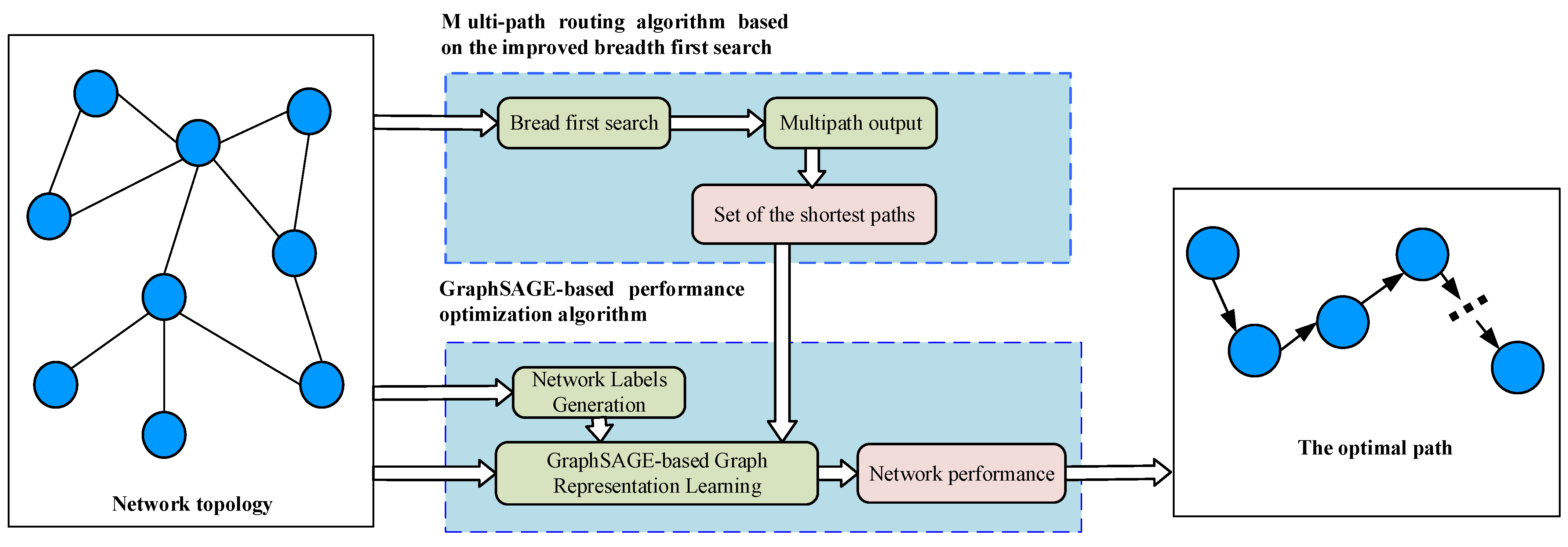
Propose a multi-path routing algorithm based on the improved breadth-first search. The algorithm can traverse the information of all neighbor nodes of the source, calculate the shortest hop count and predecessor nodes from neighbor nodes to the source, and then output all shortest paths based on this information.

(2)

Based on the multiple shortest paths found, a GraphSAGE-based performance optimization algorithm is proposed. The algorithm can generate network labels to train the GraphSAGE model. And then the network performance value of each node is obtained according to the inputting network topology, node features, and the trained GraphSAGE model. The network performance of each shortest path is composed of the sum of the network performance of each node in the path. Eventually, the path with the best network performance is selected for data transmission.

(3)

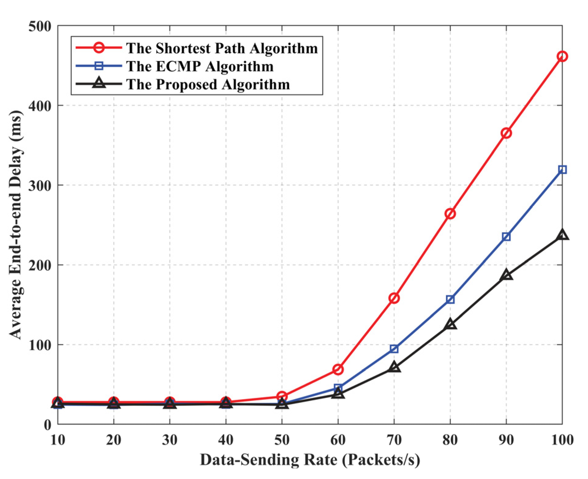
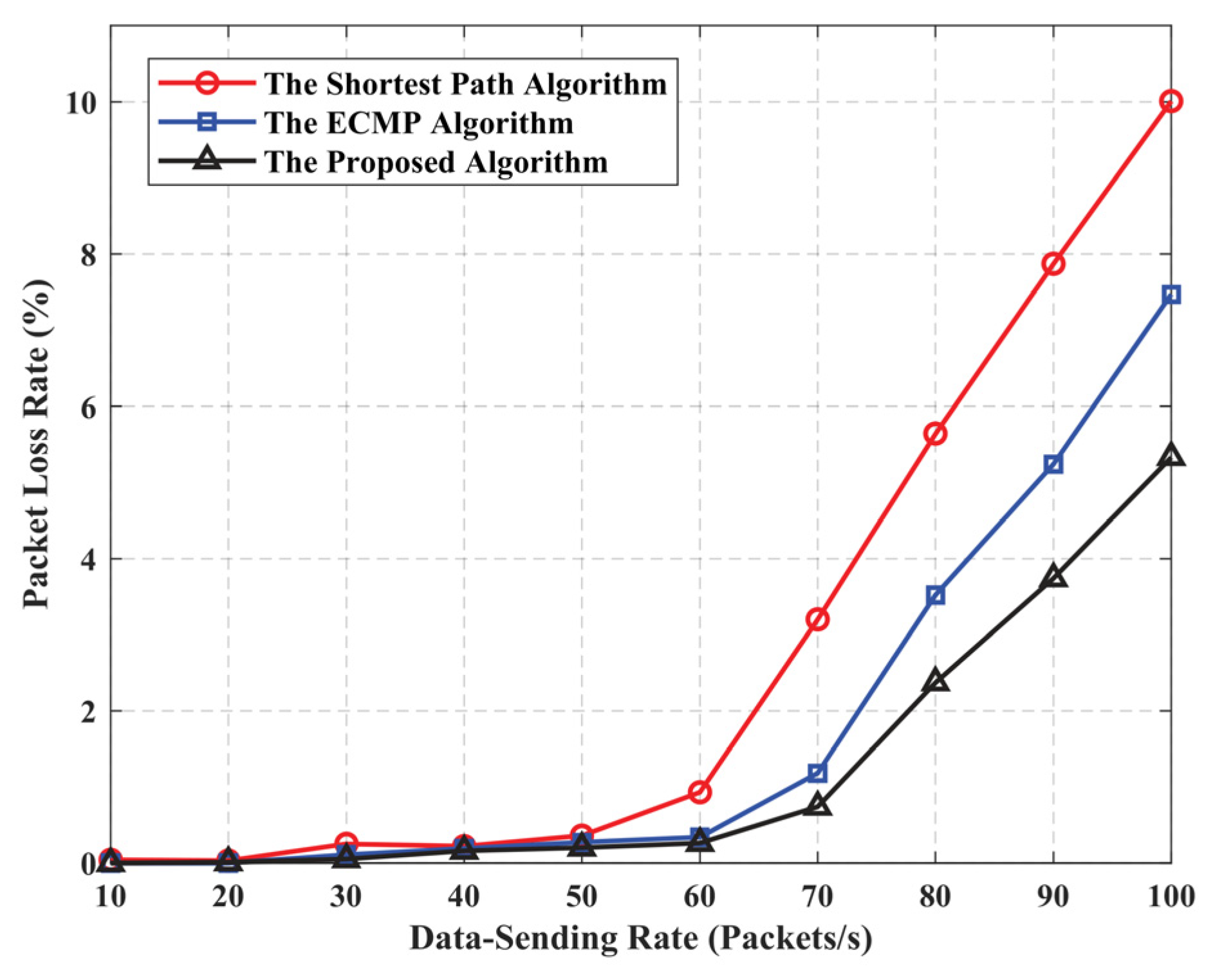
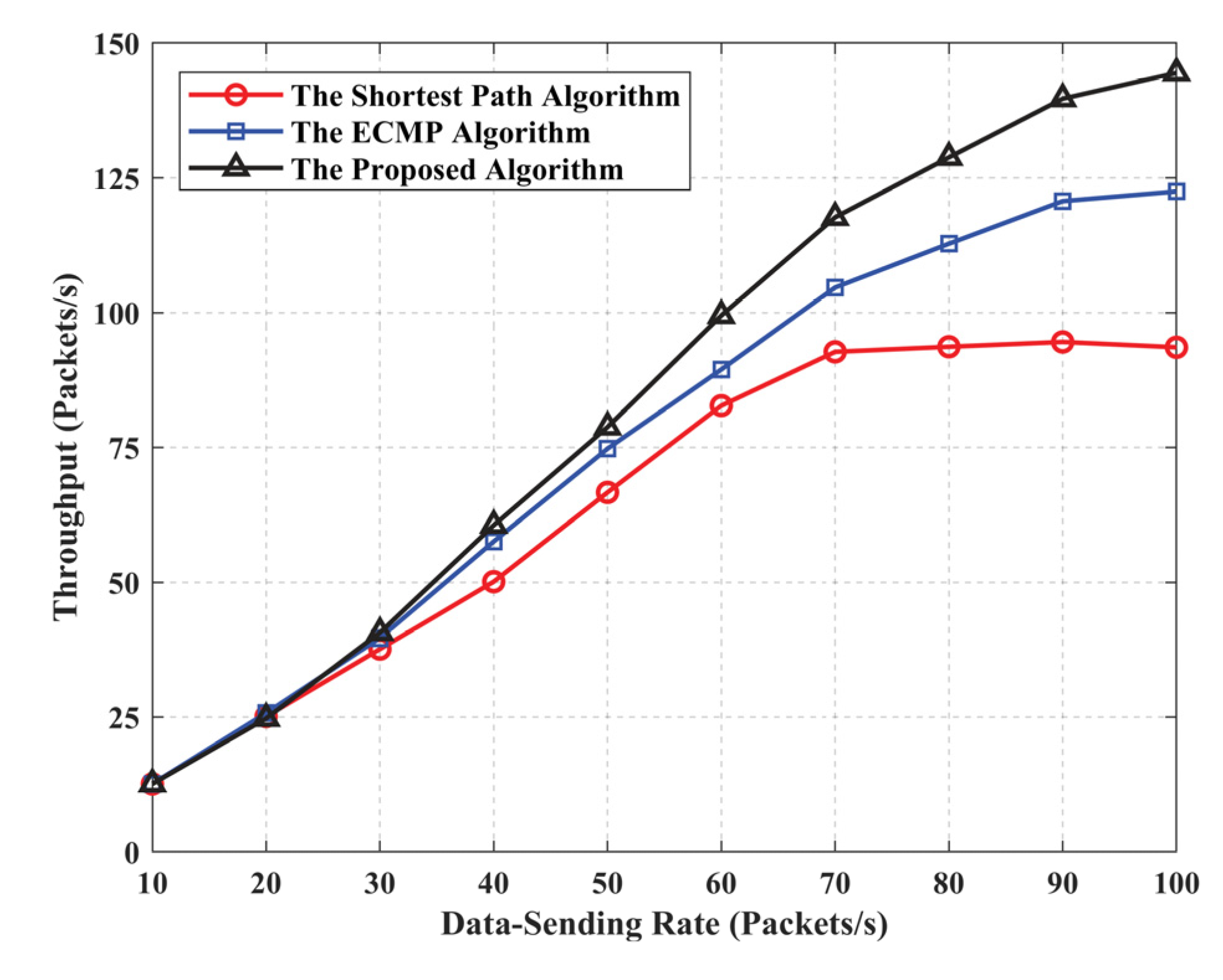
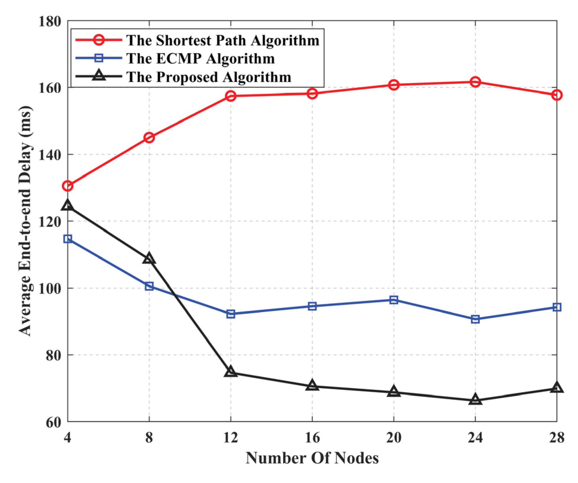
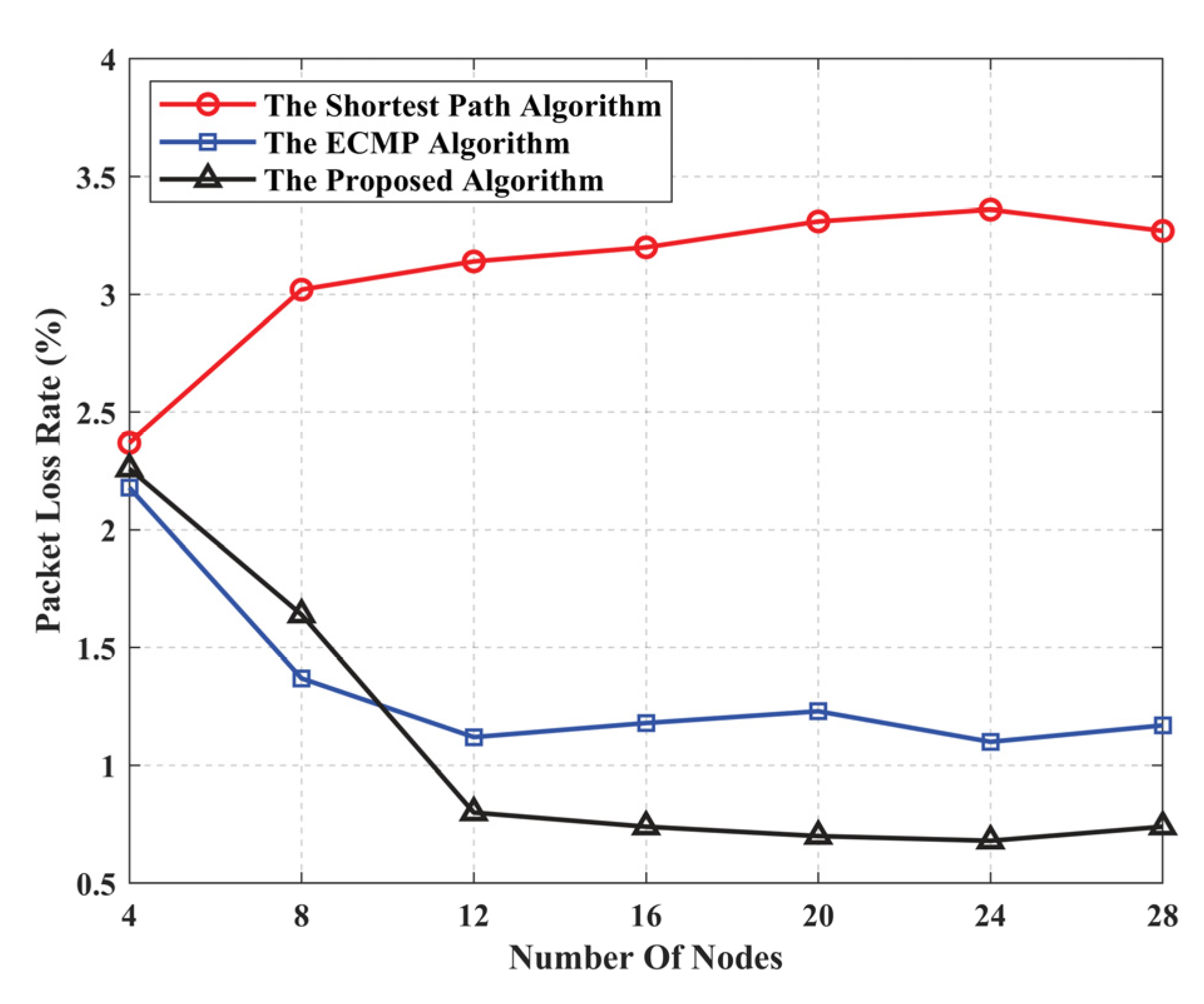
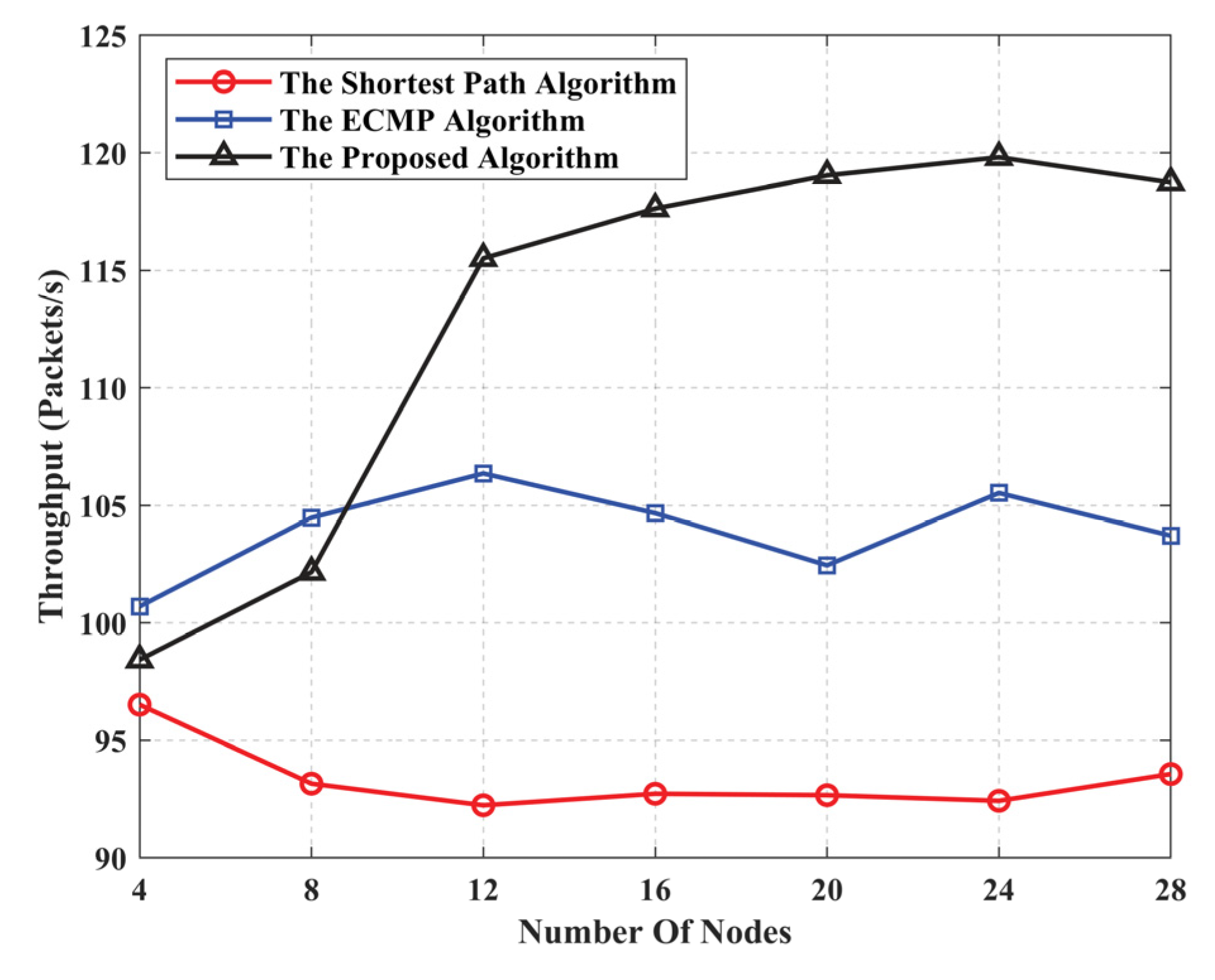
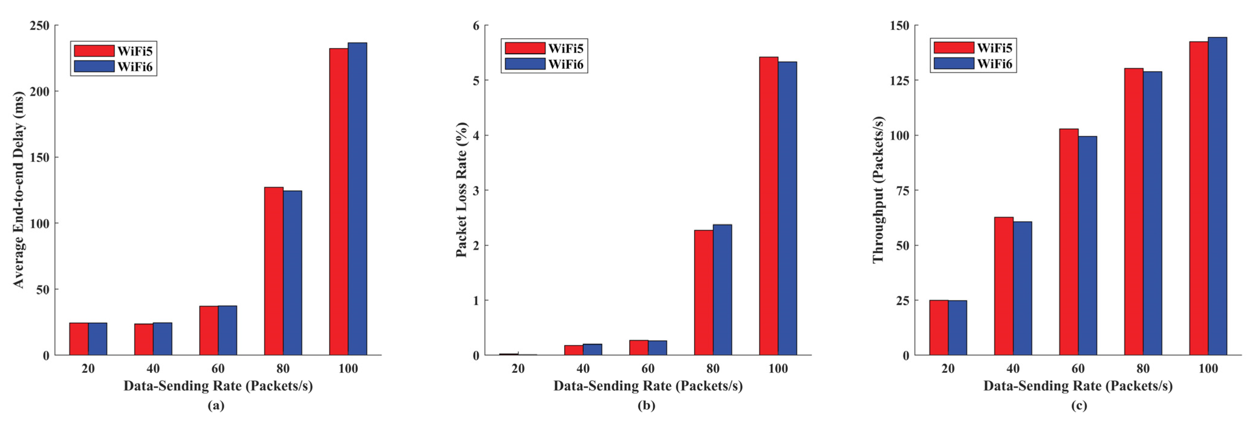
The proposed algorithm is evaluated from the effects of data sending rate, topology size, and channel environment on network performance (average end-to-end delay, packet loss rate, and throughput), respectively. The rest of the paper is organized as follows: Section 2 presents the system model. Section 3 presents the multi-path routing algorithm based on the improved breadth-first search. Section 4 presents the GraphSAGE-based performance optimization algorithm. The simulation methodology and results are shown in Section 5. Finally, Section 6 summarizes the findings of the paper.

2. System Model

This section describes the network model, the algorithm architecture, and some notations used in the algorithm.

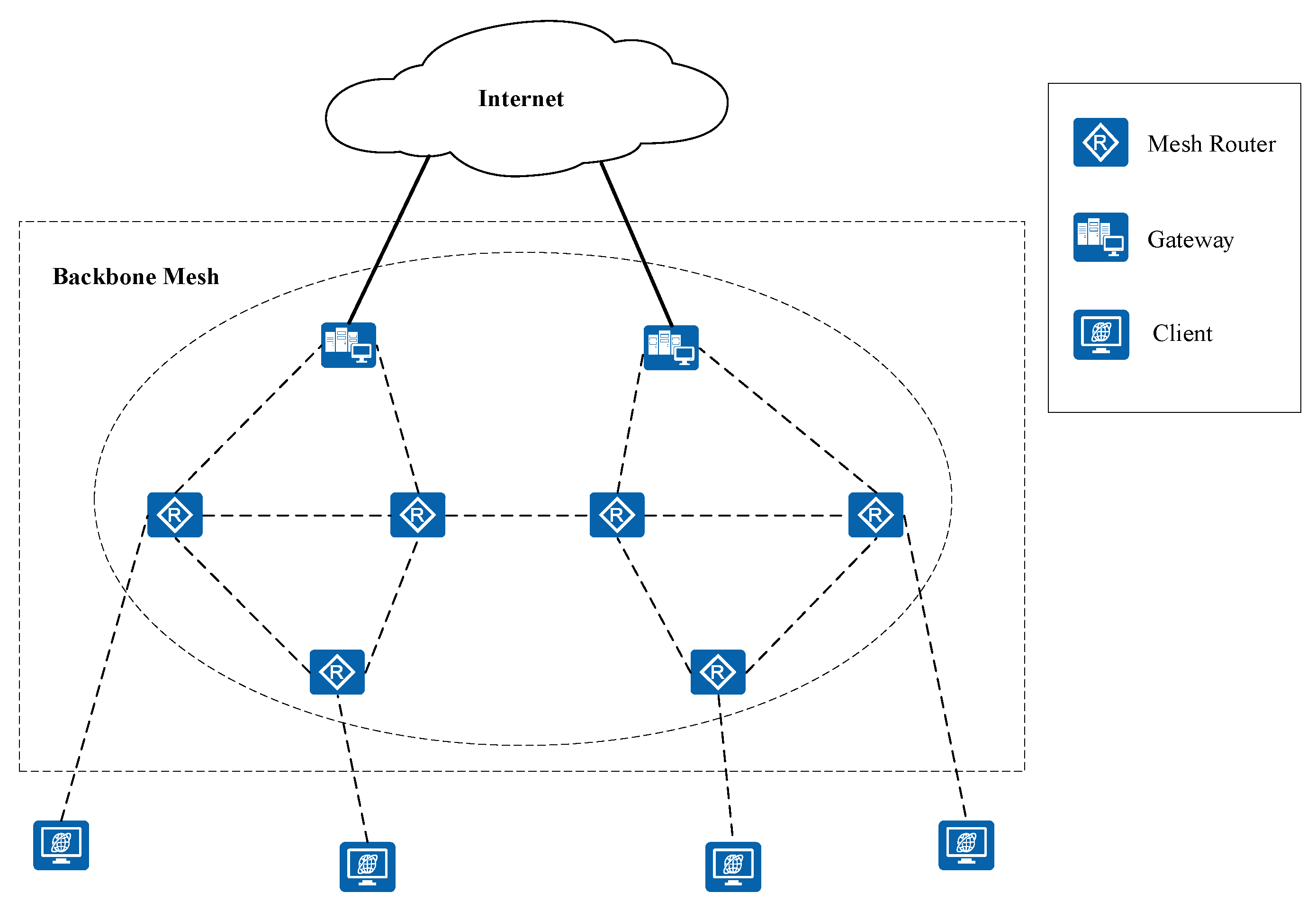
2.1. Network Model

The structure of wireless mesh networks is shown in Figure 1. which are made up of radio nodes that communicate with each other by WiFi6. As a new generation of wireless network technology, WiFi6 has the advantages of high bandwidth, low delay, and low power consumption, and is widely used in wireless mesh networks. The radio nodes include mesh clients, mesh routers, and gateways [16]. The clients communicate directly with mesh routers. And mesh routers are connected through wireless links in a self-organizing manner to form a backbone mesh network. Here, clients, mesh routers, and gateways are collectively called routing nodes. Traffic is forwarded to the gateway connected to the Internet via multiple nodes in a backbone mesh network.

In this paper, the network topology is constructed as an undirected graph $G(V,E)$. The total node set $V=\left\{v\right|v=1,2,\cdots ,N\}$ represents all routing nodes, and $N$ is the total number of nodes. The link set $E=\left\{e_{ij}\right|i,j\in V\}$ represents all links in the network. The link $e_{ij}\in E$ exists only if $d_{ij}\le R$, where $d_{ij}$ denotes the Euclidean distance between nodes $i$ and $j$, $R$ represents the maximum radio transmission range.

2.2. Architecture

According to the characteristics of WMN, this paper proposes a reliable routing algorithm that combines the improved breadth-first search and GraphSAGE to improve reliability and increase network resource utilization. As shown in Figure 2. the algorithm architecture consists of two parts: (1) All shortest paths from the source to the destination are iterated by a multi-path routing algorithm based on the improved breadth-first search. (2) The GraphSAGE-based performance optimization algorithm is used to learn the network graph information, determine the network performance of each path, and finally select the path with the best network performance for data transmission from all shortest paths. In other words, the multi-path routing algorithm based on the improved breadth-first search generates the set of candidate paths, and the GraphSAGE-based performance optimization algorithm determines the subset of the paths to be used.

2.3. Notations

• $Head$: Head node, the first element of the queue.
• $Queue$: Queue used to store neighbor nodes.
• $Visited$: Visited status, if $Visited=True$, the neighbor node has been visited and has been in the queue. Otherwise $Visited=Flase$.
• $Searched$: Searched status, if $Searched=True$, the neighbor node has already been searched, and can be skipped.
• $HopCount(v)$: The shortest hop count from node $v$ to the source.
  $FrontCount(v)$: The number of predecessor nodes of node $v$.
• $\mathrm{FrontPoint}(v)$: Set of predecessor nodes of node $v$. There are $FrontCount(v)$ elements in the set.
• $Array$: Neighbor node list used to store all neighbor nodes of the top element of the main stack.
• $Path$: Set of the shortest paths used to store the shortest paths output by multi-path routing algorithm based on the improved breadth first search.

3. Multi-Path Routing Algorithm Based on the Improved Breadth First Search

Breadth-first search algorithm (BFS) is a search algorithm that visits neighbor nodes sequentially from the source, then visits unsearched neighbor nodes sequentially layer by layer, and finally stops traversing once the destination is searched [17]. But only one shortest path is obtained, and other shortest paths cannot be output in BFS, which may result in one of the neighbor nodes of the source being used for data forwarding all the time, causing network congestion. Therefore, this paper designs a new multi-path algorithm, which is an improvement on the breadth-first search algorithm. The algorithm can continuously iterate over the link information to output all shortest paths. It has two key steps, breadth-first search, and multipath output.

3.1. Breadth-First Search

According to the collected network topology information, the connectivity between nodes in the network is represented by an adjacency matrix $A(a_{ij})$, where the elements $a_{ij}$ are defined as

$$a_{ij}=\{\begin{array}{c}1, if node i and node j are connected\hfill \\ 0, else\hfill \end{array}$$

(1)

The breadth-first search uses an adjacency matrix $A$ to traverse the information of neighbor nodes of the head node and calculate the shortest hop count and predecessor nodes from the neighbor node to the source. After all the neighbor nodes are traversed, the head node is out of the queue and a new head node is generated until the queue is empty. In this way, the shortest hop count of all nodes to the source and the predecessor nodes of each node are obtained. The flow chart of the improved breadth-first search is shown in Figure 3, and the specific steps are as follows.

Step 1: 

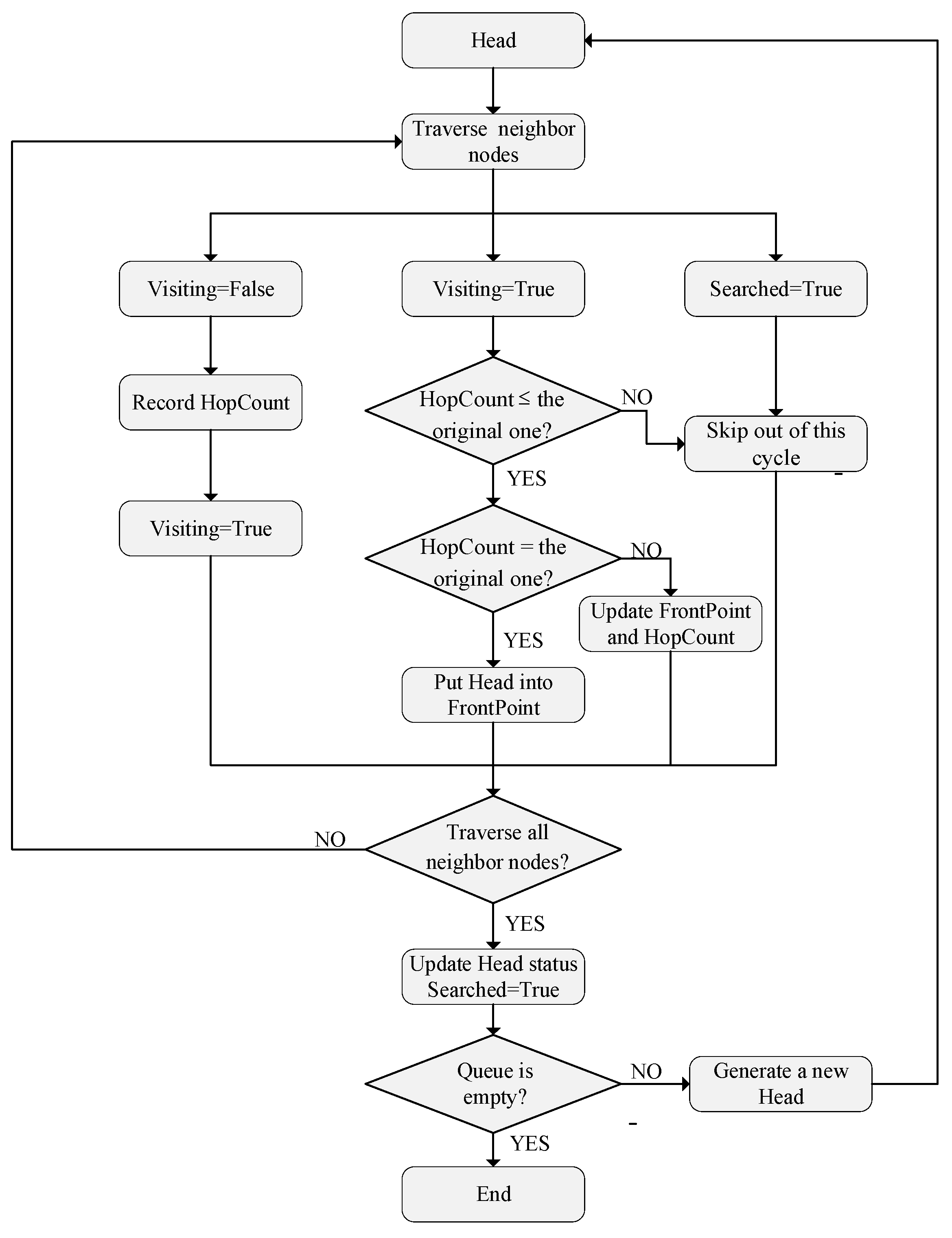
First initialize the correlation parameters, put the source $src$ as the head node $Head$ into $Queue$, set the status $Visited$ of the source to $True$, the rest of the nodes to $False$, and the status $Searched$ of all nodes to $False$. Set $HopCount(Head)$ to zero, which represents the hop count from the head node to the source is zero. Traverse adjacency matrix $A$ to find all the neighbor nodes of the head node and the address of one of the neighbor nodes is denoted by $Neighbor$. Query the current status of this neighbor node.

Step 2: 

If $Visited=False$, $HopCount(Neighbor)$ = $HopCount(Head)+1$, and the number of predecessor nodes of this neighbor node $FrontCount(Neighbor)$ is increased by one. At the same time, put the head node as the predecessor node of the current neighbor node into $\mathit{FrontPoint}(Neighbor)$. Finally, put the neighbor node in $Queue$ and set the status $Visited$ of this node to $True$.

Step 3: 

If $Visited=True$, this node is also a neighbor node of other nodes, it is necessary to compare the size of the shortest hop count from the neighbor node to the source. If the shortest hop count obtained in this loop is smaller than the original one, update $HopCount(Neighbor)$ to the shortest hop count of this loop and keep $FrontCount(Neighbor)$ unchanged. If the shortest hop count obtained in this loop is equal to the original one, $FrontCount(Neighbor)$ is increased by one. At the same time, put $Head$ as another predecessor node of the current neighbor node into $\mathit{FrontPoint}(Neighbor)$. If the shortest hop count obtained in this loop is larger than the original one, skip out of this loop.

Step 4: 

If $Searched=True$, this node has been searched, so skip out of this loop. After all neighbor nodes are traversed, update the status $Searched$ of the head node as $True$. In the end, remove the head node from $Queue$ and generate a new head node.

Step 5: 

Repeat steps 2 to 4 until $Queue$ becomes empty.

The shortest hop count from the source to each node and the predecessor nodes of each node have been obtained after a breadth-first search. Section 3.2 will use the information to output multipath.

3.2. Multipath Output

Based on $\mathit{FrontPoint}$ obtained in Section 3.1, the connecting relations of the nodes in the shortest paths are obtained. This paper introduces the shortest path adjacency matrix $A_s$. This adjacency matrix only keeps the connecting relations of the nodes that satisfy the shortest paths, which means that all paths from the source to the destination obtained through this adjacency matrix are the shortest paths. The elements of $A_s(a_{s_{ij}})$ are defined as follows, where $i,j=0,1,\cdots ,N-1$.

$$a_{s_{ij}}=\{\begin{array}{c}1, if node j\in \mathit{FrontPoint}(i)\hfill \\ 0, else\hfill \end{array}$$

(2)

By traversing the shortest path adjacency matrix $A_s$, all the shortest paths between the source to destination are obtained. This paper uses an algorithm that combines stack and loop for full traversal [18]. This algorithm requires two stacks, a main stack $Stac{k}_{main}$ to store the nodes on the path and an auxiliary stack $Stac{k}_{auxiliary}$ to store the neighbor node list $Array$ of the corresponding element of $Stac{k}_{main}$. The main and auxiliary stacks are of equal length. The algorithm is as follows (Algorithm 1):

Algorithm 1: Multipath Output Algorithm

Input:$\mathrm{The} \mathrm{shortest} \mathrm{path} \mathrm{adjacency} \mathrm{matrix} A_s$; $\mathrm{source} src$; $\mathrm{destination} dst$ Output:$\mathrm{The} \mathrm{set} \mathrm{of} \mathrm{shortest} \mathrm{paths} Path=\left\{pat{h}_i\right|i=1,2,\cdots ,m\}$ $1 \mathrm{Press} src$$\mathrm{into} \mathrm{the} \mathrm{main} \mathrm{stack} Stac{k}_{main}$. $2 \mathrm{Traverse} \mathrm{shortest} \mathrm{path} \mathrm{adjacency} \mathrm{matrix} A_s$$, \mathrm{store} \mathrm{neighbor} \mathrm{nodes} \mathrm{of} \mathrm{the} \mathrm{source} \mathrm{into} \mathrm{the} \mathrm{neighbor} \mathrm{node} \mathrm{list} Array$$, \mathrm{and} \mathrm{then} \mathrm{press} Array$$\mathrm{into} \mathrm{the} \mathrm{auxiliary} \mathrm{stack} Stac{k}_{auxiliary}$ as the top of the stack. 3 while$Stac{k}_{main}$ is not empty do $4\hspace{1em}\mathrm{Obtain} \mathrm{the} \mathrm{top} \mathrm{of} Stac{k}_{auxiliary}$$\mathrm{as} \mathrm{a} \mathrm{new} \mathrm{list} \mathrm{of} \mathrm{neighbor} \mathrm{nodes} Array$ $5\hspace{1em}\mathbf{if} Array$ is not empty then 6    $\mathrm{Obtain} \mathrm{the} \mathrm{first} \mathrm{element} \mathrm{of} Array$, press it into $Stac{k}_{main}$$, \mathrm{and} \mathrm{press} \mathrm{the} \mathrm{list} \mathrm{of} \mathrm{remaining} \mathrm{elements} \mathrm{into} Stac{k}_{auxiliary}$ 7    Query the neighbor node list of the element at the $\mathrm{top} \mathrm{of} Stac{k}_{main}$, if the list contains elements in $Stac{k}_{main}$, eliminate the duplicate elements from $\mathrm{the} \mathrm{list} \mathrm{first} \mathrm{and} \mathrm{then} \mathrm{press} \mathrm{the} \mathrm{list} \mathrm{into} Stac{k}_{auxiliary}$$; \mathrm{if} \mathrm{not}, \mathrm{press} \mathrm{the} \mathrm{list} \mathrm{into} Stac{k}_{auxiliary}$ directly $8\hspace{1em}\mathbf{else} \mathrm{Pop} \mathrm{the} \mathrm{top} \mathrm{elements} \mathrm{of} Stac{k}_{main}$$\mathrm{and} Stac{k}_{auxiliary}$ 9  end if $10\hspace{1em}\mathbf{if} \mathrm{the} \mathrm{top} \mathrm{element} \mathrm{of} Stac{k}_{main}=dst$ then $11\hspace{1em}\hspace{1em}\mathrm{Obtain} \mathrm{a} \mathrm{path} p_i=Stac{k}_{main}$$\mathrm{and} \mathrm{put} \mathrm{it} \mathrm{int} Path$ $12\hspace{1em}\hspace{1em}\mathrm{Pop} \mathrm{the} \mathrm{top} \mathrm{elements} \mathrm{of} Stac{k}_{main}$$\mathrm{an} Stac{k}_{auxiliary}$ 13 end if 14 end while $15 \mathbf{return} Path$

4. GraphSAGE-Based Performance Optimization Algorithm

According to the multi-path routing algorithm proposed in Section 3, all the shortest paths have been obtained from the source to the destination. To avoid network congestion and improve transmission efficiency, we prioritize the path with good network performance from them for data transmission. Therefore, a GraphSAGE-based performance optimization algorithm is further proposed, which selects the path with the best network performance by the node network performance based on the network topology and node features. The algorithm consists of two key steps, network label generation, and GraphSAGE-based graph representation learning.

4.1. Network Labels Generation

Usually, data of the collected network feature only contains node network features such as traffic, delay, and packet loss rate, and lacks labels of node network performance, which makes it difficult to train the GraphSAGE model. In order to train the GraphSAGE model in a supervised manner, the collected data need to be discretized to generate network performance labels, so this paper introduces fuzzy c-means (FCM) clustering algorithm. The FCM algorithm has been widely used in neural networks, clustering, classification, and image analysis in recent years [19]. Compared with hard clustering which strictly classifies the samples into a certain class, fuzzy clustering establishes an uncertain description of the samples to the class and reflects the sample status more objectively.

Node features at each moment of the network are collected to form a network feature dataset $X_{train}$ that contains $n$ samples. If the samples are divided into $l$ classes, the corresponding cluster centers are $\{c_1,c_2\cdots c_l\}$. The objective function of the FCM algorithm can be written as

$$\min J={\displaystyle \sum _{i=1}^c{\displaystyle \sum _{j=1}^n{u}_{ij}{}^m{d}_{ij}{}^2}}$$

(3)

where $u_{ij}$ denotes the membership value of the sample $j$ to the cluster center $i$;$m$ denotes the fuzzy exponent, $m\in [1,\infty )$, and $d_{ij}$ denotes the Euclidean distance between the sample $j$ and cluster center $i$.

According to Lagrange’s theorem, the necessary condition to minimize $J$ is

$$u_{ij}=\frac{1}{{{\displaystyle \sum _{k=1}^c(\frac{d_{ij}}{d_{ik}})}}^{\frac{2}{m-1}}}$$

(4)

$$c_i=\frac{{\displaystyle \sum _{j=1}^n{u}_{ij}{}^m{x}_j}}{{\displaystyle \sum _{j=1}^n{u}_{ij}{}^m}}$$

(5)

The values of Equations (5) and (6) are iterated until the value of $J$ is less than the set threshold or the number of iterations reaches the maximum number of iterations. In order to determine the optimal number of clusters $l_{best}$, the Fuzzy Partition Coefficient (FPC) proposed in [20] is used to evaluate the cluster validity. The value of FPC is between zero and one, the closer to one means the better quality of clustering and the higher similarity of samples within the class. The calculation formula of FPC is as follows:

$$FPC=\frac{1}{n}{\displaystyle \sum _{j=1}^n{\displaystyle \sum _{i=1}^n{u}_{ij}^2}}$$

(6)

Since the network topology proposed in this paper contains two types of nodes: routing nodes and link nodes, the number of clusters $l$ must be greater than two. And in order to enhance the differentiation of network performance, this paper takes $l=4~8$.

After clustering by the FCM algorithm, although data of the network feature have been classified into $l_{best}$ classes, it is still unable to determine which class has better network performance. Network feature contains several metrics such as traffic, delay, packet loss rate, etc., and there is often a situation in that different metrics cannot be compared uniformly in the process of network performance judgment. For example, class A has several feature metrics that are better than class B, but class B has several metrics that are better than class A, which makes it difficult to determine which class is better in terms of network performance. This paper uses a multi-metrics comprehensive evaluation method [21], which combines metrics of several network features to form a comprehensive metric as the reflection of network performance.

Due to the different dimensions of network feature metrics, it is unable to directly process the network feature data numerically, so it is necessary to convert the data to nondimensional values. In this paper, the normalization method is used to process network feature metrics. Traffic is a benefit index, and the larger the value, the better the network performance. Transmission delay and packet loss rate are cost metrics, and the smaller the value, the better the network performance. Assume that $q_{ij}$ denotes the value of metric $j$ of the sample $i$, $q_j{}^{\min }$ and $q_j{}^{\max }$ denote the minimum and maximum values of metric $j$, respectively, where $i=1,2,\cdots ,n; j=1,2,\cdots ,m$. value as $l_{best}$, and obtain the cluster center $\{c_1,c_2,\cdots ,c_{l_{best}}\}$. At this point, $X_{train}$ has been divided into $l_{best}$ classes. The normalization process of the benefit metrics is as follows:

$$d_{ij}=\frac{q_{ij}-q_j{}^{\min }}{q_j{}^{\max }-q_j{}^{\min }}$$

(7)

The normalization process of the cost metrics is as follows:

$$d_{ij}=\frac{q_j{}^{\max }-q_{ij}}{q_j{}^{\max }-q_j{}^{\min }}$$

(8)

The weighted average method is used to calculate the network performance value $performance$, which is used to evaluate the network performance, and the larger the value the better the network performance. The network performance value can be written as:

$${performance}_i={\displaystyle \sum _{j=1}^m{w}_j{d}_{ij}}$$

(9)

where $w_j$ represents the weight of metric $j$, ${\displaystyle \sum _{j=1}^m{w}_j=1}$, and $w_j$ can be set with different weight values according to specific requirements. According to the study of the influencing factors of network performance in [22], we select three important network performance metrics, traffic, transmission delay, and packet loss rate, and set the weight values $w=(0.2,0.35,0.45)$. The specific process of generating labels for the network feature dataset is as follows:

Step 1: 

Randomly initialize the membership value $u_{ij}$, and the fuzzy coefficient is generally set to 2 by default [23]. Use the FCM algorithm to iterate parameters on the network feature dataset $X_{train}$ to obtain the cluster center $\left\{c_1,c_2,\cdots ,c_l\right\}$ and fuzzy partition coefficient FPC.

Step 2: 

Repeat Step 1 with a different number of clusters $l$, record the number of clusters with the largest FPC value as $l_{best}$, and obtain the cluster center $\{c_1,c_2,\cdots ,c_{l_{best}}\}$. At this point, $X_{train}$ has been divided into $l_{best}$ classes.

Step 3: 

Take the average of the network feature vectors of the network feature dataset by category to obtain $l_{best}$ network feature vectors, and calculate their corresponding network performance value $performance$. Rank the network performance classes according to the network performance value $performance$, the larger the value the better the network performance, thus the network performance can correspond to the cluster categories.

Step 4: 

According to the cluster centers obtained from Step 2 and the relationship between network performance and cluster categories obtained from Step 3, label the node feature vectors $\left\{x_v\right|v=0,\cdots ,N-1\}$ by network performance value $performance$, which provides conditions for the supervised training of the GraphSAGE model.

4.2. GraphSAGE-Based Graph Representation Learning

GraphSAGE is used to learn the network topology $G(V,E)$ and node features $\left\{x_v,v=0,\cdots ,N-1\right\}$. GraphSAGE aggregates the features of neighbor nodes to generate the vector representation of the target node, which is used for the following node classification task. This paper selects three attributes of traffic, transmission delay, and packet loss rate as node feature vectors, then $x_v$ can be written as:

$$x_v=[Q_v,D_v,L_v]$$

(10)

where $Q_v$ denotes the traffic (in this paper, the packet delivery rate is used to express the traffic); $D_v$ denotes the transmission delay; $L_v$ denotes the packet loss rate.

As shown in Figure 4, the process of GraphSAGE to generate node vector representations can be divided into three steps.

(1)

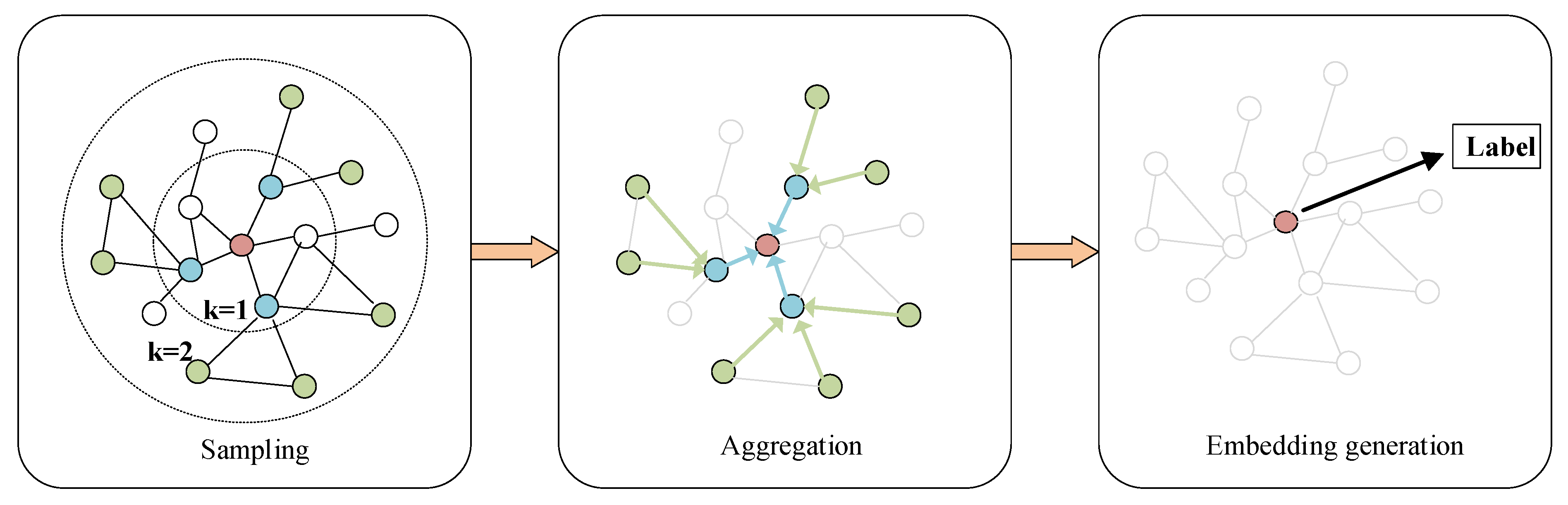
Sampling: The target node is selected by random walk, and then the neighbor nodes of the target node are sampled. The number of neighbors sampled in each hop is $S_i,i=1,2,\cdots ,K$. If the number of neighbor nodes is less than $S_i$, a resampling method with put back is used. If the number of neighbor nodes is greater than $S_i$, a negative sampling method without put back is used. $K$ represents the search depth, and according to the study of [15], when $K=2$, GraphSAGE can get excellent performance, so $K$ is set as 2. When $K=2$, $S_1=3$, $S_2=7$, the sampling process is shown in the sampling section of Figure 4.

(2)

Aggregation: GraphSAGE aggregates the information of neighbor nodes at each layer by $K$ aggregator functions and updates the target node’s own node information. In this paper, the Mean aggregator is used to obtain the aggregated features of neighbor nodes at each layer. GraphSAGE then splices the feature representation of the target node at layer $k-1$ with the aggregated features of the neighbor nodes in layer $k$, and eventually uses the nonlinear activation function to obtain the vector representation of the target node of layer $k$. The process of neighbor nodes aggregation is as follows:

$$h_{N(v)}^k\leftarrow Mean(\{h_u^{k-1},u\in N(v)\})$$

(11)

where $N(v)$ denotes the set of neighbor nodes of node $v$; $h_u^{k-1}$ donates the feature representation of the neighbor node $u$ at layer $k-1$; $h_{N(v)}^k$ donates the aggregated features of neighbor nodes of node $v$ at layer $k$. The process of node $v$ at layer $k$ to generate vector representations is as follows:

$$h_v^k\leftarrow \sigma (W^k\cdot CONCAT(h_v^{k-1},h_{N(v)}^k))$$

(12)

where $CONCAT$ uses the residual concatenation to linearly superimpose each feature vector; $W^k$ is the weight matrix to be learned; $\sigma$ is a nonlinear activation function; $\{h_v^k,k=1,2,\cdots ,K\}$ represents the vector representation of node $v$ at layer $k$. When $k=0$, the vector representation of node $v$, is defined as the input feature of node $v$, i.e., $h_v^0=x_v$.

(3)

Embedding generation: The vector representation of each node in layer $K$ in the graph structure is obtained as the final vector representation $z_v$ for the following node classification task. The process is as follows:

$$z_v\leftarrow h_v^K$$

(13)

GraphSAGE embedding generation algorithm describes the process of GraphSAGE to generate node vector representations, which is as follows (Algorithm 2).

Algorithm 2: GraphSAGE Embedding Generation Algorithm [15]

Input:$\mathrm{Undirected} \mathrm{graph} G(V,E)$$; \mathrm{node} \mathrm{features} \left\{x_v,v=0,\cdots ,N-1\right\}$$; \mathrm{sampling} \mathrm{number} S_k$, $k$$=k=1,\cdots ,K$; search depth $K$$; \mathrm{weight} \mathrm{matrix} W^k,k=1,\cdots ,K$; nonlinear activation function $\sigma$$; \mathrm{mean} \mathrm{aggregator} \mathrm{function} Mean$ Output:$\mathrm{Vector} \mathrm{representations} z_v,v=0,\cdots ,N-1$ $1 \mathrm{Initialization}:h_v{}^0\leftarrow x_v,v=0,\cdots ,N-1$; $2 \mathbf{for} k=1,\cdots ,K$do $3\hspace{1em}\mathbf{for} v=0,\cdots ,N-1$do $4\hspace{1em}\hspace{1em}{h}_{N(v)}^k\leftarrow Mean(\{h_u^{k-1},u\in N(v)\})$ $5\hspace{1em}\hspace{1em}{h}_v^k\leftarrow \sigma (W^k\cdot CONCAT(h_v^{k-1},h_{N(v)}^k))$ 6  end $7\hspace{1em}{h}_v^k\leftarrow h_v^k/{\Vert h_v^k\Vert }_2$ 8 end $9 z_v^k\leftarrow h_v^K$

After obtaining the vector representations of nodes, it is also necessary to learn the parameters of the GraphSAGE model. Weight matrix $W^k$ is the core of GraphSAGE, which contains the mapping relationship of the aggregated features of neighbor nodes to the vector representations of the target node. Therefore, the main process of parameter learning is to train a good weight matrix. And the network labels generated in Section 4.1 allow for supervised learning of the parameters. The cross-entropy function is used as the loss function for the node classification task [24]. The loss function is as follows:

$$Loss=-{\displaystyle \sum _{v\in y_{Label}}^{}{\displaystyle \sum _{i=1}^c{y}_{vi}\ln }}{z}_{vi}$$

(14)

where $y_{Label}$ represents the set of nodes with labels; $y_{vi}$ represents the network labels after One-Hot encoding; $l$ represents the number of network labels classes. The vector representation $z_{vi}$ of node $v$ is obtained through forward propagation, and then the gradient descent method is used to perform backpropagation to update $W^k$ and parameters in the aggregation function until the loss value does not change. At this point, the model has converged and can correspond well to the nodes in the network topology to the network performance.

The trained GraphSAGE model can directly follow Algorithm 2 to complete feature aggregation in the face of new topologies and node features, yielding the results of network performance classification of nodes.

Assume that the multiple shortest paths iterated by the multi-path routing algorithm are $Path=\{p_1,p_2,\cdots ,p_m\}$, and each path consists of several nodes. The class of each node in the network topology can be obtained by inputting the network topology and node feature information into the trained GraphSAGE model. After knowing the class to which the node belongs, the corresponding network performance value of the node can also be known. The network performance of each shortest path can be defined as the sum of the network performance of each node in the path, then the network performance of the shortest path $i$ can be written as:

$$N{P}_i={\displaystyle \sum _{v\in p_i}^{}performanc{e}_v}$$

(15)

where $performanc{e}_v$ represents the network performance of node $v$; $v$ is a node in the path $p_i$. The network performance of each path is calculated according to Equation (15). The path with the largest value of $NP$ is the optimal path $p_{bset}$.

5. Simulation

This section describes the experimental environment and the model training process and evaluates the performance of the proposed algorithm based on the simulation results.

5.1. Experimental Environment and Model Training Process

The network simulations are performed in $NS3$. In the simulations, the maximum radio transmission range and the interference range is set to 300 m and 500 m, respectively. The log-distance path loss model is used as the propagation model, which is suitable for outdoor propagation such as in urban areas, and the path loss exponent is set to 3 [25]. The constant speed propagation delay model is used as the delay model. Unless specifically stated, the simulations are performed in a 16 Mesh nodes topology within an area of $1000 \mathrm{m} \times 1000 \mathrm{m}$ and the node transmission power is set to 23.0306 dB. The distribution of the nodes is shown in Figure 5. WiFi6 is used as the physical layer protocol, which operates in a 5GHz frequency band. The traffic is sent from the source using the User Datagram Protocol (UDP) and the packet size is 1024 bytes.

In the experiments, the implementation of the GraphSAGE model is based on Python 3.8 and the deep learning framework PyTorch. The network topology of 16 nodes is first simulated in $NS3$, 30 routing schemes that are randomly generated and traffic is sent at 10 different rates for each routing scheme. 1000 pieces of network performance data are collected for training. Based on the combination of each routing scheme and sending rate, $NS3$ is used to generate network performance metrics such as traffic, transmission delay, and packet loss rate. Then the FCM algorithm of Section 4.1 is used to iterate the clustering centers of the network performance dataset and correspond the network performance to the clustering categories one by one. Finally, the network labels are generated based on the feature vectors of the nodes in the topology and the GraphSAGE model is trained in a supervised manner. During the training process, the number of iterations of the GraphSAGE is set to 3000, the learning rate $lr$ is set to 0.003 and the neural network uses the Adam optimizer and the Relu activation function. In addition, the number of first-order neighbor nodes is set to 4 and the number of second-order neighbor nodes is set to 8.

5.2. Algorithm Performance Evaluation

The evaluation consists of two parts: (1) The GraphSAGE-based performance optimization algorithm can effectively evaluate the network performance and optimize the selection of transmission paths. (2) The actual performance of the multi-path reliable routing algorithm for wireless mesh networks is evaluated and proven to improve the network performance. The average of 10 runs of the program is used as the simulation results. During each run, randomly select several source-destination node pairs from the network topology for packet transmission, record the network performance metrics such as end-to-end delay, packet loss rate, and throughput, and take the arithmetic average of the simulation data.

This section first proves that the GraphSAGE-based performance optimization algorithm can effectively evaluate the network performance and optimize the selection of transmission paths. The available bandwidth (avail-bw) of an end-to-end path is defined as the residual capacity at the path’s bottleneck, which represents the maximum additional load that the path can carry before saturation [26]. It is often applied as a network performance metric for path selection. After outputting all shortest paths by the multi-path routing algorithm based on the improved breadth-first search, we use path selection based on the available bandwidth method and the GraphSAGE-based performance optimization algorithm for optimal path selection, respectively, and compare the network performance between the two selection methods at different data sending rates. The experimental results are shown in Figure 6. The figure shows that there is little difference between the two methods when the data-sending rate is low. This is because the amount of data has not reached the bandwidth capacity. When the data sending rate is higher, the GraphSAGE-based performance optimization algorithm has a lower average end-to-end delay and packet loss rate, and greater throughput. The GraphSAGE-based performance optimization algorithm considers multiple network performance metrics and can select transmission paths more accurately. Overall, the GraphSAGE-based performance optimization algorithm can effectively evaluate the network status, optimize the selection of transmission paths, and improve the network performance.

In order to verify the actual performance of the proposed GraphSAGE-based multi-path reliable routing algorithm, the proposed algorithm is evaluated from the effects of data sending rate, topology size, and channel environment on the network performance, respectively. The traditional shortest path routing algorithm and the Equal-Cost Multi-Path routing (ECMP) [27] are selected as the comparison algorithms to evaluate the performance of the proposed algorithm.

To study the effect of data sending rate on algorithm performance, the data sending rate is increased from 10 packets/s to 100 packets/s. The experimental results are shown in Figure 7, Figure 8 and Figure 9. Figure 7 explains the average end-to-end delay at different data-sending rates. The figure indicates that the average end-to-end delay is increasing as the data-sending rate increases. Figure 8 illustrates that as the data-sending rate increases, the packet loss rate also increases. Figure 9 shows the relationship between throughput and data sending rate, where throughput increases and then levels off as the data sending rate increases. When the data sending rate is low, there is no significant difference in the performance of the three algorithms because the amount of data has not yet reached the bandwidth capacity and the network status is good. However, when the data sending rate is higher, the proposed algorithm outperforms the two comparison algorithms in terms of network performance metrics such as average end-to-end delay, packet loss rate, and throughput. This is because the traditional shortest path routing algorithm can select only one shortest path for data transmission, which is prone to network congestion. Although the EMCP algorithm can perform multi-path transmission, it only spreads the traffic to different paths for transmission, which is likely to worsen the congestion for the paths that have already been congested. Instead, the proposed algorithm can not only obtain all the shortest paths from the source to the destination, avoiding the limitation that the traditional shortest path algorithm can select only one path for transmission but also dynamically select the optimal path according to the network performance, effectively alleviating network congestion. Moreover, as the data-sending rate increases, the performance improvement of the proposed algorithm becomes larger and larger, which effectively improves the network performance, reduces average end-to-end delay and packet loss rate, and increases throughput.

To study the effect of topology size on algorithm performance, the data sending rate is fixed at 70 packets/s and the number of topological nodes is increased from 4 to 28. The experimental results are shown in Figure 10, Figure 11 and Figure 12. Figure 10 explains the average end-to-end delay with a different number of topological nodes. The figure illustrates that as the number of topological nodes increases the average end-to-end delay of the shortest path algorithm first increases and then levels off, while the ECMP algorithm and the proposed algorithm first decrease and then level off. Figure 11 shows the packet loss rate with a different number of topological nodes. In this figure, the variation of packet loss rate with topological nodes follows the same trend as the average end-to-end delay in Figure 10. Figure 12 indicates that the throughput of the shortest path algorithm decreases first and then levels off as the number of topological nodes increases. The results show that the shortest path routing algorithm gives the worst network performance due to selecting only one shortest path for data transmission, which is prone to network congestion. When the number of topological nodes is small, the available shortest paths are also very few, so the proposed algorithm cannot exert its ability to dynamically select the optimal path and the network performance is poor. However, the ECMP algorithm can spread the traffic to different paths for transmission, with better network performance, which is more suitable for simple topologies with a small number of nodes. When the number of topological nodes is bigger, the network performance of the proposed algorithm is better and less volatile compared with the ECMP algorithm. The proposed algorithm analyses multi-attribute parameters such as traffic, packet loss rate, and transmission delay, which can dynamically select the optimal path according to the network performance, effectively alleviate network congestion and improve network performance.

To study the effect of channel environment on network performance, WiFi5, and WiFi6, the two latest WiFi protocols, are used as the physical layer protocol of WMN for simulation, respectively. In terms of modulation mode, WiFi6 supports 1024-QAM and WiFi5 supports 256-QAM. In the simulation, the two protocols both operate in a 5GHz frequency band. As shown in Figure 13, there is no significant difference in network performance for the two-channel environments at different data-sending rates. This shows that the proposed algorithm has good performance in different channel environments and can be applied to various channel environments.

6. Conclusions

This paper proposes a reliable routing algorithm to address the problems that traditional routing algorithms have low network resource utilization and are difficult to guarantee the reliability of transmission in real networks. The algorithm consists of a multi-path routing algorithm based on the improved breadth-first search and a GraphSAGE-based performance optimization algorithm, which can output all shortest paths and select the path with the best network performance for data transmission based on the real-time network status. Simulation results show that the proposed algorithm outperforms the traditional shortest path routing algorithm and ECMP algorithm in the face of complex networks, and can effectively improve network performance, reduce delay and packet loss rate, and increase throughput. As the data-sending rate increases, the performance improvement of the scheme given by the proposed algorithm compared to the comparison algorithms becomes larger and larger. When the data sending rate reaches 100 packets/s, the proposed algorithm reduces the average end-to-end delay by 48.8% and 35.1%, the packet loss rate by 46.75% and 28.65%, and increases the throughput by 54.3% and 18.0% compared with the shortest path algorithm and ECMP algorithm, respectively. Although the proposed algorithm can greatly optimize the network performance, the time complexity of the algorithm is not considered. As the network topology becomes more and more complex, the resource consumption of the routing algorithm becomes a serious issue. Therefore, in our future research, we intend to optimize the time complexity of the algorithm to reduce resource consumption.

References

- Dey, S.; Sarmah, H.; Samantray, S.; Divakar, D.; Pathak, S. Energy efficiency in wireless mesh networks. In Proceedings of the 2010 IEEE International Conference on Computational Intelligence and Computing Research, Coimbatore, India, 28–29 December 2010; pp. 1–4. [Google Scholar]
- Rozner, E.; Seshadri, J.; Mehta, Y.; Qiu, L. SOAR: Simple opportunistic adaptive routing protocol for wireless mesh networks. IEEE Trans. Mob. Comput. 2009, 8, 1622–1635. [Google Scholar] [CrossRef]
- Vijayakumar, K.; Ganeshkumar, P.; Anandaraj, M. Review on routing algorithms in wireless mesh networks. Int. J. Comput. Sci. Telecommun. 2012, 3, 87–92. [Google Scholar]
- Wang, L.; Zhang, L.; Shu, Y.; Dong, M. Multipath source routing in wireless ad hoc networks. In Proceedings of the 2000 Canadian Conference on Electrical and Computer Engineering. Conference Proceedings. Navigating to a New Era (Cat. No. 00TH8492), Halifax, NS, Canada, 7–10 May 2000; pp. 479–483. [Google Scholar]
- Jia, D.; Zou, S.; Li, M.; Zhu, H. Adaptive multi-path routing based on an improved leapfrog algorithm. Inf. Sci. 2016, 367, 615–629. [Google Scholar]
- Guo, X.; Wang, F.; Liu, J.; Cui, Y. Path diversified multi-QoS optimization in multi-channel wireless mesh networks. Wirel. Netw. 2014, 20, 1583–1596. [Google Scholar] [CrossRef]
- Pan, C.; Liu, B.; Zhou, H.; Gui, L. Multi-path routing for video streaming in multi-radio multi-channel wireless mesh networks. In Proceedings of the 2016 IEEE International Conference on Communications (ICC), Kuala Lumpur, Malaysia, 22–27 May 2016; pp. 1–6. [Google Scholar]
- Liu, C.; Xu, M.; Geng, N.; Zhang, X. A survey on machine learning based routing algorithms. J. Comput. Res. Dev. 2020, 57, 671–687. [Google Scholar]
- Yun, W.-K.; Yoo, S.-J. Q-learning-based data-aggregation-aware energy-efficient routing protocol for wireless sensor networks. IEEE Access 2021, 9, 10737–10750. [Google Scholar] [CrossRef]
- Tang, J.; Mihailovic, A.; Aghvami, H. Constructing a DRL decision making scheme for multi-path routing in All-IP access network. In Proceedings of the GLOBECOM 2022–2022 IEEE Global Communications Conference, Rio de Janeiro, Brazil, 4–8 December 2022; pp. 3623–3628. [Google Scholar]
- Modi, T.M.; Swain, P. Intelligent routing using convolutional neural network in software-defined data center network. J. Supercomput. 2022, 78, 13373–13392. [Google Scholar] [CrossRef]
- Zheng, X.; Huang, W.; Li, H.; Li, G. Research on Generalized Intelligent Routing Technology Based on Graph Neural Network. Electronics 2022, 11, 2952. [Google Scholar] [CrossRef]
- Xu, Z.; Tang, J.; Meng, J.; Zhang, W.; Wang, Y.; Liu, C.H.; Yang, D. Experience-driven networking: A deep reinforcement learning based approach. In Proceedings of the IEEE INFOCOM 2018-IEEE Conference on Computer Communications, Honolulu, HI, USA, 16–19 April 2018; pp. 1871–1879. [Google Scholar]
- Kipf, T.N.; Welling, M. Semi-supervised classification with graph convolutional networks. arXiv 2016, arXiv:1609.02907. [Google Scholar]
- Hamilton, W.; Ying, Z.; Leskovec, J. Inductive representation learning on large graphs. Adv. Neural Inf. Process. Syst. 2017, 30, 1–11. [Google Scholar]
- Sarkar, S.K.; Basavaraju, T.G.; Puttamadappa, C. Ad Hoc Mobile Wireless Networks: Principles, Protocols and Applications; Auerbach Publications: Boca Raton, FL, USA, 2007. [Google Scholar]
- Priyana, R.; Handayani, E.T.E. Perancangan Game “Heroes Surabaya†Sebagai Edukasi Pengetahuan Sejarah Menggunakan Algoritma BFS Berbasis Android. JIMP (J. Inform. Merdeka Pasuruan) 2019, 4, 1–7. [Google Scholar] [CrossRef]
- Li, H. Binary Tree’s Recursion Traversal Algorithm and Its Improvement. J. Comput. Commun. 2016, 4, 42–47. [Google Scholar] [CrossRef]
- Nayak, J.; Naik, B.; Behera, H. Fuzzy C-means (FCM) clustering algorithm: A decade review from 2000 to 2014. In Computational Intelligence in Data Mining—Volume 2, Proceedings of the International Conference on CIDM, Orlando, FL, USA, 9–12 December 2014; Springer: Berlin/Heidelberg, Germany, 2015; pp. 133–149. [Google Scholar]
- Trauwaert, E. On the meaning of Dunn’s partition coefficient for fuzzy clusters. Fuzzy Sets Syst. 1988, 25, 217–242. [Google Scholar] [CrossRef]
- Meng, J.; Tang, W.; Tang, H.; Xu, W.; Wang, M. A Comprehensive Evaluation System Urban Distribution Network. In Proceedings of the 2018 IEEE 4th Information Technology and Mechatronics Engineering Conference (ITOEC), Chongqing, China, 14–16 December 2018; pp. 1139–1143. [Google Scholar]
- Hanemann, A.; Liakopoulos, A.; Molina, M.; Swany, D.M. A study on network performance metrics and their composition. Campus-Wide Inf. Syst. 2006, 23, 268–282. [Google Scholar] [CrossRef]
- Pei, H.-X.; Zheng, Z.-R.; Wang, C.; Li, C.-N.; Shao, Y.-H. D-FCM: Density based fuzzy c-means clustering algorithm with application in medical image segmentation. Procedia Comput. Sci. 2017, 122, 407–414. [Google Scholar] [CrossRef]
- Yang, P.; Tong, L.; Qian, B.; Gao, Z.; Yu, J.; Xiao, C. Hyperspectral image classification with spectral and spatial graph using inductive representation learning network. IEEE J. Sel. Top. Appl. Earth Obs. Remote Sens. 2020, 14, 791–800. [Google Scholar] [CrossRef]
- Phunthawornwong, M.; Pengwang, E.; Silapunt, R. Indoor location estimation of wireless devices using the log-distance path loss model. In Proceedings of the TENCON 2018–2018 IEEE Region 10 Conference, Jeju, Republic of Korea, 28–31 October 2018; pp. 499–502. [Google Scholar]
- Jain, M.; Dovrolis, C. Path selection using available bandwidth estimation in overlay-based video streaming. Comput. Netw. 2008, 52, 2411–2418. [Google Scholar] [CrossRef]
- Zhang, H.; Guo, X.; Yan, J.; Liu, B.; Shuai, Q. SDN-based ECMP algorithm for data center networks. In Proceedings of the 2014 IEEE Computers, Communications and IT Applications Conference, Beijing, China, 20–22 October 2014; pp. 13–18. [Google Scholar]
Disclaimer/Publisher’s Note: The statements, opinions and data contained in all publications are solely those of the individual author(s) and contributor(s) and not of MDPI and/or the editor(s). MDPI and/or the editor(s) disclaim responsibility for any injury to people or property resulting from any ideas, methods, instructions or products referred to in the content. |
© 2023 by the authors. Licensee MDPI, Basel, Switzerland. This article is an open access article distributed under the terms and conditions of the Creative Commons Attribution (CC BY) license (https://creativecommons.org/licenses/by/4.0/).
Share and Cite
Lu, P.; Jing, C.; Zhu, X. GraphSAGE-Based Multi-Path Reliable Routing Algorithm for Wireless Mesh Networks. Processes 2023, 11, 1255. https://doi.org/10.3390/pr11041255
Lu P, Jing C, Zhu X. GraphSAGE-Based Multi-Path Reliable Routing Algorithm for Wireless Mesh Networks. Processes. 2023; 11(4):1255. https://doi.org/10.3390/pr11041255
Chicago/Turabian StyleLu, Pan, Chuanfang Jing, and Xiaorong Zhu. 2023. "GraphSAGE-Based Multi-Path Reliable Routing Algorithm for Wireless Mesh Networks" Processes 11, no. 4: 1255. https://doi.org/10.3390/pr11041255