Optimization of Flow and Mixing in a Venturi Tube Mixer with a Two-Step Method Using Numerical Simulation

Abstract

To achieve efficient mixing in a Venturi tube mixer (VTM), an optimization with a two-step method for this mixing device based on a Venturi tube (VT) was carried out using numerical simulation. Firstly, the effects of the structural parameters on the flow in VT were revealed, and the optimized configuration was determined for the following VTM. Subsequently, by introducing a jetting tube, the suction capacity, energy consumption and mixing quality were used to evaluate the performance of VTM under various configurations and operating conditions. According to the effects of the structural parameters on the mixing quality of VTM, an empirical formula for mixing quality with structural parameters was proposed. Finally, an optimized VTM was proposed. This work can provide a valid suggestion for the design and optimization of such a mixing device.

1. Introduction

A confined impinging jet reactor is a typical mixing device in a process requiring quick mixing, which is due to the intensified local energy dissipation, resulting in excellent mass transfer capacity [1,2,3]. However, the operation of confined impinging jet reactors usually requires streams with equal momentum or jet diameter, or the deviation of stagnation point will lead to an obvious decline in micro-mixing, which is not beneficial to a quick or instantaneous reaction [4]. Apparently, the confined impinging jet reactor is not easily applicable for mixing between unequal flows. For example, in the Beckmann rearrangement reaction, an important step in the production of caprolactam, the flow ratio between the cyclohexanone oxime and the strongly acidic can be as low as 0.7 [5], where the confined impinging jet rector will not be so appropriate.

Hence, a reactor which can be applied to the mixing with unequal flows is required in such a process, such as the Venturi tube mixer (VTM) [6]. The very first VTM was proposed and designed by Eric Haliburn, based on the Venturi effect, to rapidly mix cementitious grout [7]. Then, it was widely used in the production of liquid insecticides and the irrigation of agriculture [8]. A further understanding of the flow and mixing characteristics of VTM can promote its industrial value.

In the investigation of the flow and mixing characteristics in VTM, two typical flow phenomena in VTM are noteworthy, including the Venturi effect induced by fluid flow in the Venturi tube (VT) and the cross-flow generated by passive or active jetting fluid into the VT. Much research has been carried out on these two aspects in recent decades. Goharzadeh et al. [9] investigated the velocity field in VT using Particle Image Velocimetry (PIV), and the results showed the pressure drop caused by viscosity mainly existed at the divergent region outlet. Vijay et al. [10] numerically simulated the velocity, pressure and turbulence kinetic energy distributions in the VT, and found at most 5% relative error between the simulated and experimental results, indicating the accuracy and feasibility of Computational Fluid Dynamics (CFD). Sanghani et al. [11] explored the effects of convergent ratio, length of throat, convergent angle and divergent angle on the pressure distribution in the VT using numerical simulation, and the convergent ratio was found to be the most influential factor among all parameters. Shi et al. [12] explored fluid flow in the VT by simulation and experiment, and the convergent angle was found to greatly affect the cavitation phenomena in the VT. As for the cross-flow, Luo et al. [13] used Planar Lase-Induced Fluorescence (PLIF) and the Large Eddy Simulation (LES) method to investigate the mixing process of cross-flow and revealed the effect of the interaction between two fluids on flow vortex. Kartaev et al. [14] investigated macroscopic mixing in the cross-flow by both experiment and numerical simulation and calculated the axial penetration depth of countercurrent jetting flow.

In addition to the research method, many researchers have concentrated on how the structural and operating conditions affect the flow and mixing characteristics in VTM. Li et al. [15] researched the hydraulic characteristics in VTM using CFD, and the results showed that the pressure at the throat region is more difficult to accurately predict than that at other regions, resulting in the requirement of refined mesh at the throat region. Simpson et al. [16] investigated the cavitation characteristics of VTM with different operating conditions. The effect of throat length, convergent angle and geometric parameters on the occurrence and degree of cavitation were quantitatively discussed. Sundararaj et al. [17,18] investigated the effects of jetting angle and operating conditions on the mixing characteristics of VTM, and the results showed that increasing the jetting angle and velocity ratio of jetting flow to motive flow can promote the mixing quality. Wang et al. [19] researched the flow field in VTM using PIV, and the results revealed that with the increase in jetting flow rate, reverse flow will appear in the downstream near the wall. Manzano et al. [20] used the CFD method to investigate the relationship between the configuration of VTM and pressure drop, which showed that the diameter of the throat was an important factor affecting the pressure drop.

However, the present research is mainly focused on the flow characteristics inside the VTM without the mixing, along with a few works on the optimization of VTM structure and understanding the relationship between the structural characteristics and the resulting flow and mixing behavior. In the present work, the CFD method will be used to reveal how structural configurations affect the flow and mixing in the VTM. Before the optimization of VTM, firstly, two typical phenomena, namely Venturi flow and cross-flow, are simulated with different meshing schemes and turbulence models. By comparing the simulated results with experimental and theoretical results, a suitable meshing scheme and a turbulence model in simulating the flow in the VT and VTM are determined. Secondly, the effect of structural parameters on the flow in VT are investigated, which includes the convergent ratio, length-diameter ratio of the throat, convergent angle and divergent angle. In the research of VTM, a jetting tube is added at the throat region of previously optimized VT to construct a VTM. Then, the research focuses on the effect of structural parameters and operating conditions on the flow and mixing characteristics in VTM, including the pore-throat diameter ratio, jetting angle, jetting position ratio and so on. Finally, a flow optimized and lower energy consumption VTM configuration is proposed.

Hence, the highlights of this work are as follows: firstly, we compare the accuracy and feasibility of different turbulence models; then, these are employed to optimize the configuration of this mixing device from VT to VTM using a two-step method, with comprehensive structural analysis, which provides a meaningful guide for the design of such a mixing device.

2. Geometry of Venturi Tube Mixer and Numerical Simulation Method

2.1. Geometry of Venturi Mixer

There are generally four regions in a Venturi tube mixer (VTM), namely the convergent region, throat region, divergent region and jetting region, as shown in Figure 1, where it is the Venturi tube (VT) if there is no jetting region.

In the operation of VTM, fluid A (motive flow or motive stream) flows from the convergent region to the divergent region through the throat region; meanwhile, fluid B (jetting flow or jetting stream) is injected from the jetting region, and then there is the mixture stream A + B flowing out of the VTM. If the jetting flow B is sucked into the throat region due to the pressure difference between the throat and jetting entrance, it is called a passive operation; when extra energy is inputted for fluid B, it is an active operation. For convenience, Figure 1 shows all the nomenclatures representing key dimensions of the VTM. An additional straight tube, whose length is 10 times the throat region diameter d, is added at convergent inlet and divergent outlet to ensure the sufficient development of turbulence.

2.2. Governing Equations in Numerical Simulation

The mixing of two or more fluid streams is the main operation purpose in a VTM. In this work, those equations are solved using ANSYS Fluent 2020R1, based on the finite volume method. The mathematical equations governing the flow and mixing are below.

2.2.1. Fluid Flow

In this work, incompressible Newtonian fluid, water at room temperature, is used as the material. The continuity equation and momentum equation are described below.

$$\nabla \cdot \overrightarrow{u}=0$$

(1)

$$\frac{Du}{D\theta }=f_{\mathrm{B}}-\frac{1}{\rho }\nabla p+\upsilon {\nabla }^2\overrightarrow{u}$$

(2)

where $\overrightarrow{u}$ is the velocity vector, θ is the time, f_B is the mass force acting on the fluid per unit mass, ρ is the fluid density, P is the pressure, υ is the fluid kinematic viscosity.

2.2.2. Fluid Mixing

In describing the mixing process between two miscible fluids, species transport is a common model. For species i in the mixing, the conservation equation is described below.

$$\frac{\partial (\rho {\phi }_{\mathrm{i}})}{\partial t}+\nabla ·(\rho {\phi }_{\mathrm{i}}u)=\nabla ·(D_{\mathrm{m}}\rho \nabla {\phi }_{\mathrm{i}})+S_{{}_{\mathrm{i}}}$$

(3)

where φ_i is the mass fraction of species i, D_m is the diffusion rate of species i, S_i is the source term of species i. There is S_i = 0 when species i is not consumed or generated by reaction in the system.

In this work, the fluids A and B described in Figure 1 are both water but are marked with different labels to distinguish their concentrations.

2.3. Boundary Condition and Solution Strategy

In this work, there are several types of boundary conditions, where the boundary for the incoming fluid was mainly the velocity inlet, and the exit for the fluid was mainly the pressure outlet according to the specific pressure conditions in the VTM. The entire solid wall in the simulated domain was set as the no-slip wall condition.

In this work, all the simulations were carried out in pressure-based and steady states. The solution method was the SIMPLE algorithm with second-order upwind for the momentum equation, first-order upwind for the turbulent kinetic energy and turbulence dissipation rate, and second-order for the pressure. Convergence criteria for all simulation runs was 10⁻⁵.

2.4. Mesh Sensitivity Analysis

In this work, according to the research scheme, there are mainly two aspects in the flow and mixing characteristics of VTM, including the flow in VT and the mixing induced from the cross-flow, where the cross-flow phenomenon needs refined mesh due to highly turbulent shearing. Therefore, there were two tests in the mesh sensitivity analysis.

2.4.1. Mesh Sensitivity of Venturi Tube

In this section, a 3D model of the Venturi tube was established based on the model of Caetano et al. [21], of which the dimensional details of this Venturi tube are shown in

Table 1. Dimensional details of Venturi tube from Caetano et al. [21].

	Din, mm	Dout, mm	d, mm	lcon, mm	lthr, mm	ldiv, mm	α, °	β, °
Value	32	32	20	60	20	50	11.4	13.7

.

In this work, all meshes are structured meshes generated in the software ICEM. There were five meshing schemes in the mesh sensitivity analysis, where the total number of grid cells were about 0.02 million, 0.09 million, 0.13 million, 0.29 million and 0.58 million, respectively. In this section, the fluid velocity at the convergent inlet boundary and the pressure at the divergent outlet boundary are v_con = 1.106 m/s and P_div = 6.2 × 10⁴ Pa, respectively.

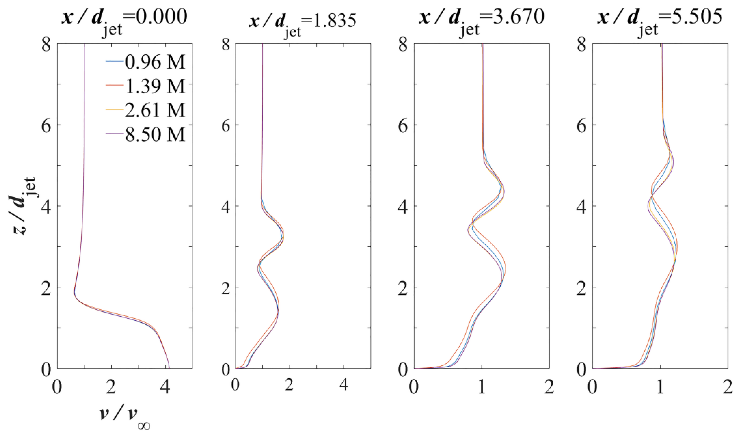
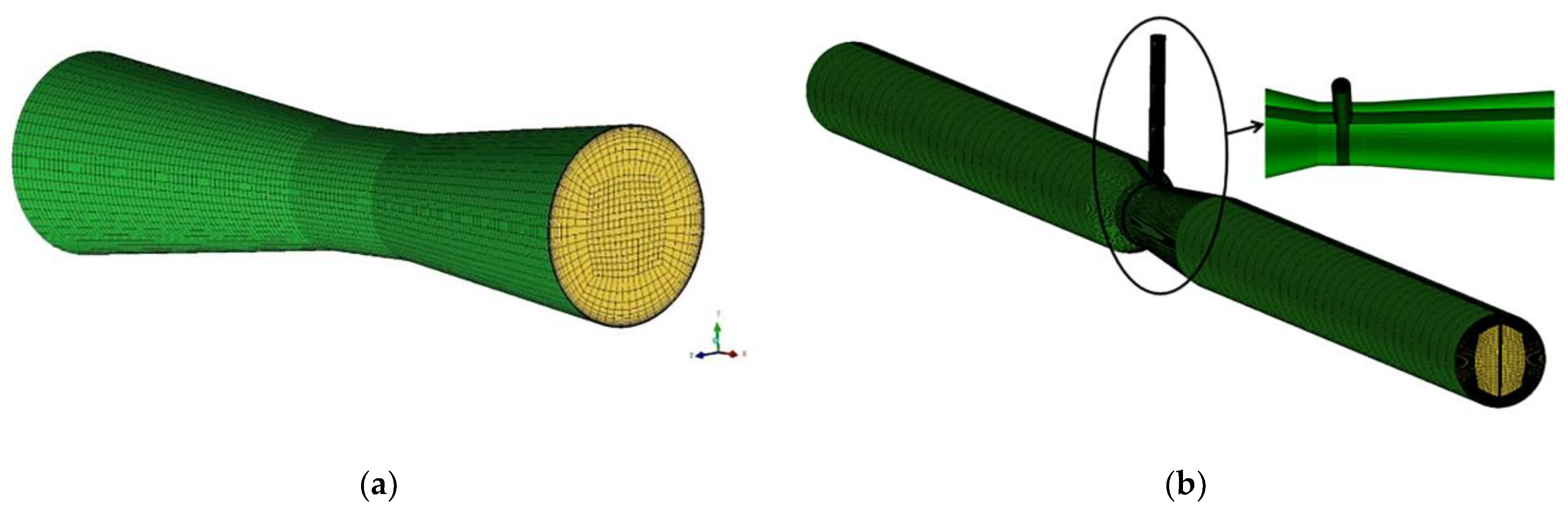
2.4.2. Mesh Sensitivity of Cross-Flow

Figure 2a,b shows a typical schematic diagram of cross-flow and the corresponding 3D model. In this cross-flow, the motive stream flows into the cubic domain from left to right; meanwhile, a jetting stream is injected from the jetting tube, which is the same as the experimental device by Sherif [22]. The dimensional details are shown in

Table 2. Dimensional details of cross-flow in the mesh sensitivity analysis.

	L, mm	H, mm	W, mm	djet, mm	ljet, mm	ljet-in, mm
Value	175.768	166.08	110.72	13.84	138.4	37.368

. Four meshing schemes were used in this test, with grid cells numbering about 0.96 million, 1.39 million, 2.61 million and 8.5 million, respectively. The values of the boundary conditions are given in

Table 3. Boundary conditions of cross-flow in the mesh sensitivity analysis.

	v∞, m/s	vjet, m/s	P∞, Pa
Value	0.35	1.155	0

.

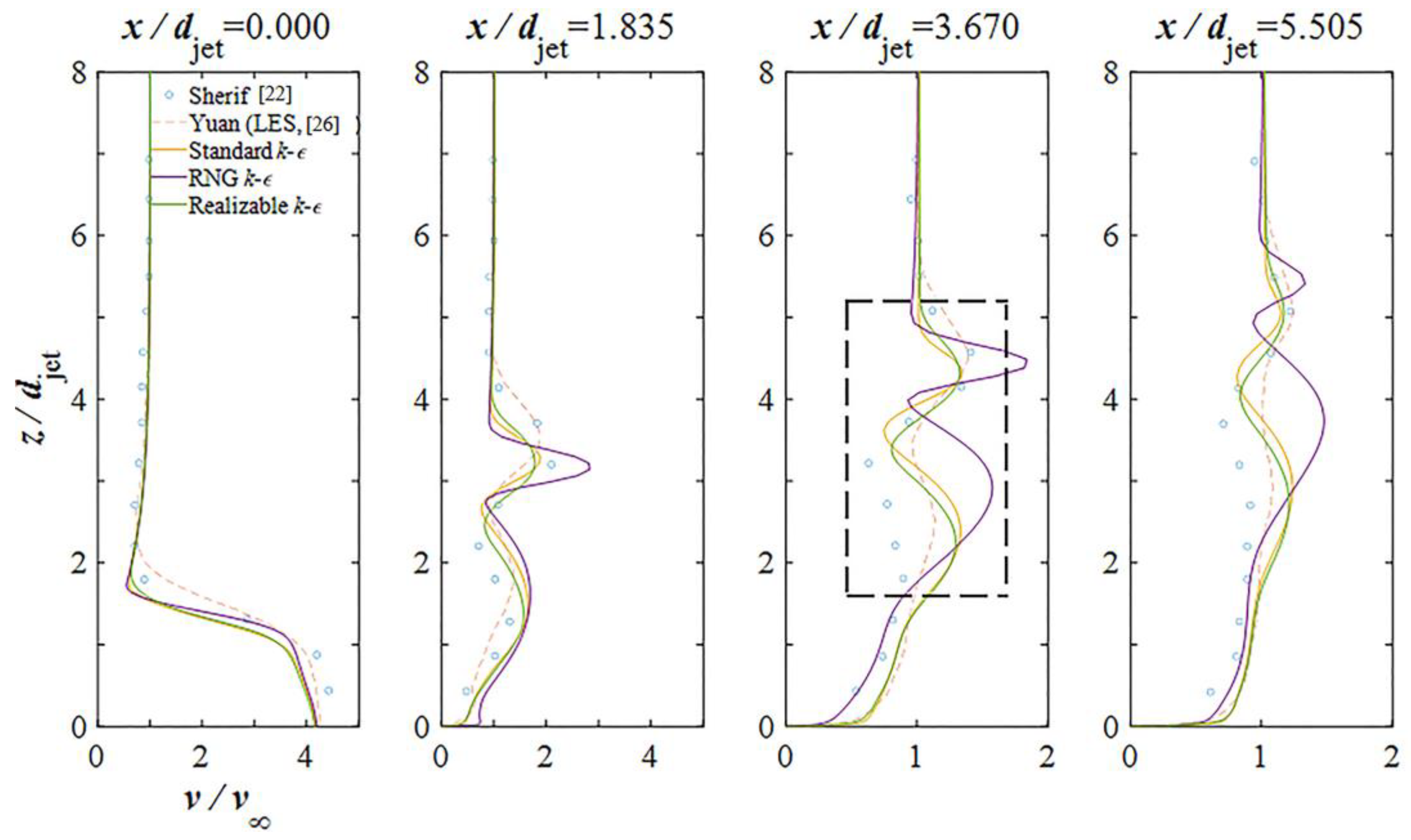
2.5. Evaluation and Selection of Turbulence Model

In the numerical simulation of fluid flow, an appropriate turbulence model is vital for describing the turbulence characteristics, where the RANS (Reynolds-Averaged Navier-Stokes) method is popular in the design of industrial devices due to its relatively low computational resource requirement and high efficiency. In the RANS method, standard $k$-$\epsilon$, RNG $k$-$\epsilon$ and Realizable $k$-$\epsilon$ are three typical models, which should be evaluated before the numerical investigation of VT and VTM.

In this section, the selection of the turbulence model is divided into two parts, namely VT and cross-flow. With regard to the selection of the turbulence model in the simulation of VT, the configuration of VT is the same as that in the mesh sensitivity analysis (Section 2.4.1). The boundary conditions are given in

Table 4. The boundary condition value details of VT in the turbulence model selection.

vcon, m/s	Re	Pdiv, ×103 Pa	vcon, m/s	Re	Pdiv, ×103 Pa
0.207	6552	6	0.691	21,842	26
0.276	8737	6	0.76	24,026	30
0.346	10,921	8	0.829	26,210	36
0.415	13,105	10	0.898	28,394	42
0.484	15,289	14	0.968	30,578	48
0.553	17,473	18	1.037	32,762	54
0.622	19,657	22	1.106	34,947	62

.

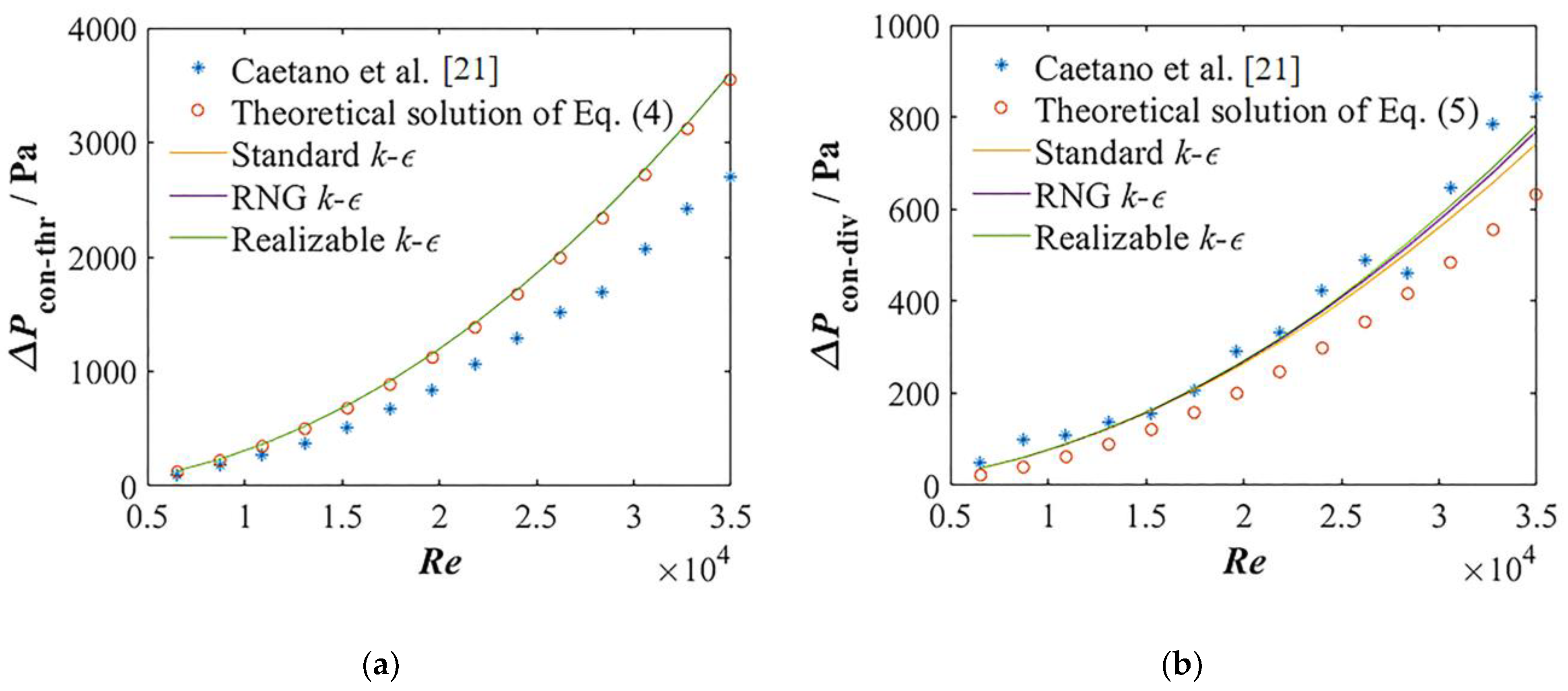
The simulated pressure drop along the VT is compared with that of the theoretical value and the literature from Caetano et al. [21] under different Reynolds numbers. The theoretical value of the pressure drop and the Reynolds number can be calculated, respectively, using Equations (4), (5) and (7).

$$\Delta P_{\mathrm{con}-\mathrm{thr}}=((K_1+1)v_{\mathrm{thr}}^2-v_{\mathrm{con}}^2)\frac{\rho }{2}$$

(4)

$$\Delta P_{\mathrm{con}-\mathrm{div}}=(K_1{v}_{\mathrm{thr}}^2+K_2{(v_{\mathrm{div}}-v_{\mathrm{thr}})}^2)\frac{\rho }{2}$$

(5)

$$v_{\mathrm{con}}=\frac{d^2}{D_{\mathrm{in}}^2}{v}_{\mathrm{thr}}=\frac{D_{\mathrm{out}}^2}{D_{\mathrm{in}}^2}{v}_{\mathrm{div}}$$

(6)

$$Re=\frac{\rho D_{\mathrm{in}}{v}_{\mathrm{con}}}{\mu }$$

(7)

where ΔP_con-thr and ΔP_con-div are the pressure difference between P_con and P_thr, P_con and P_div, respectively. K₁ and K₂ are the local pressure loss coefficients of the convergent region and the divergent region, respectively, where K₁ = 0.04 and K₂ ≈ 0.32 for β = 13.7° [23], v_con, v_div and v_thr are the fluid velocities at the convergent inlet, divergent outlet and throat out boundaries, respectively. The energy loss caused by viscous resistance can be ignored because the VT is short.

As for the turbulence model in the simulation of cross-flow, the physical geometry and the boundary conditions are both the same as that in the mesh sensitivity analysis.

2.6. Numerical Simulation Schemes of VT and VTM

An efficient VTM is desired, and in this work, there are two steps in the optimization of VTM. The parameters, which are to be optimized in this work, are the core structures of VT and VTM, including the convergent ratio, the length-diameter ratio, the convergent and divergent angles, the pore-throat diameter ratio and the jetting angle. The convergent ratio (γ₁ = d/D_in) presents the compressed degree of fluid flowing from the convergent region to the throat region, thereby affecting the pressure drop between the convergent and throat regions of VT. The length-diameter ratio (δ = l_thr/d) can affect the residence time of flow in the throat region. The convergent angle (α) and divergent angle (β) define the intensification of flow in the VT being compressed and developed. The pore-throat diameter ratio has an effect on the flow resistance of the jetting tube and then affects the suction capacity of VTM. The change of jetting angle can affect the impingement intensification between jetting flow and motive flow, thereby affecting the mixing quality and energy consumption. The jetting position ratio determines the position where jetting flow and motive flow begin to mix. In addition, the number of jetting influences the flow rate of jetting directly, then it affects the mixing quality. Firstly, the influences of the convergent ratio (γ₁ = d/D_in), length-diameter ratio of throat (δ = l_thr/d), convergent angle (α) and divergent angle (β) on the flow in VT are briefly discussed to access an optimized configuration of VT. The structural parameters in the optimization of VT are shown in

Table 5. Structural parameters in the optimization of VT.

Din, mm	Dout, mm	γ1	δ	α, °	β, °
32	32	0.500 *	0.6	8	6
		0.556	0.8	10	8
		0.625	1 *	11.4 *	10
		0.714	1.2	14	12
		0.833	1.4	16	13.7 *
				18	16
				20	18
				22
				28
				40

Note: * represents the initial structural parameters of VT.

.

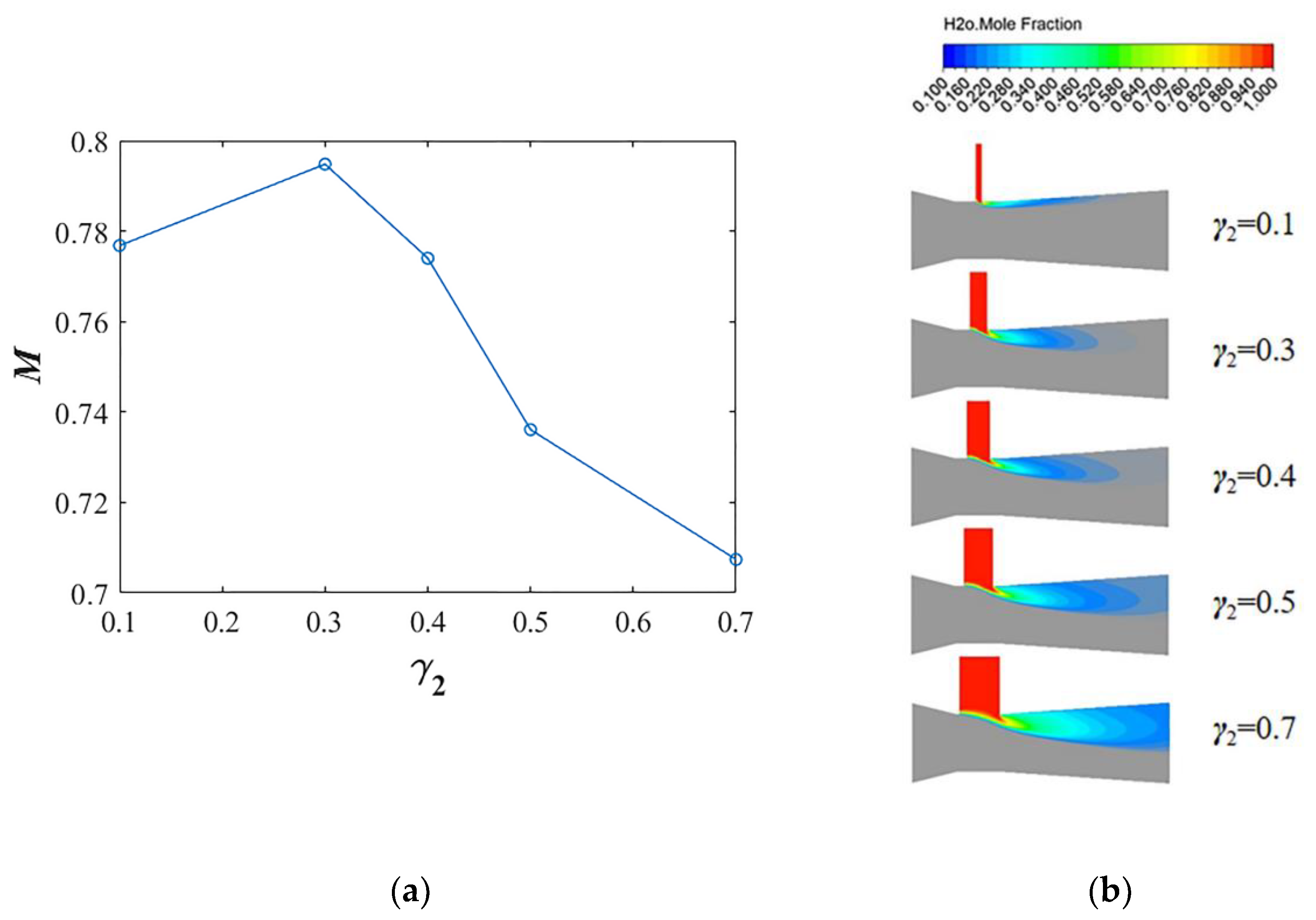
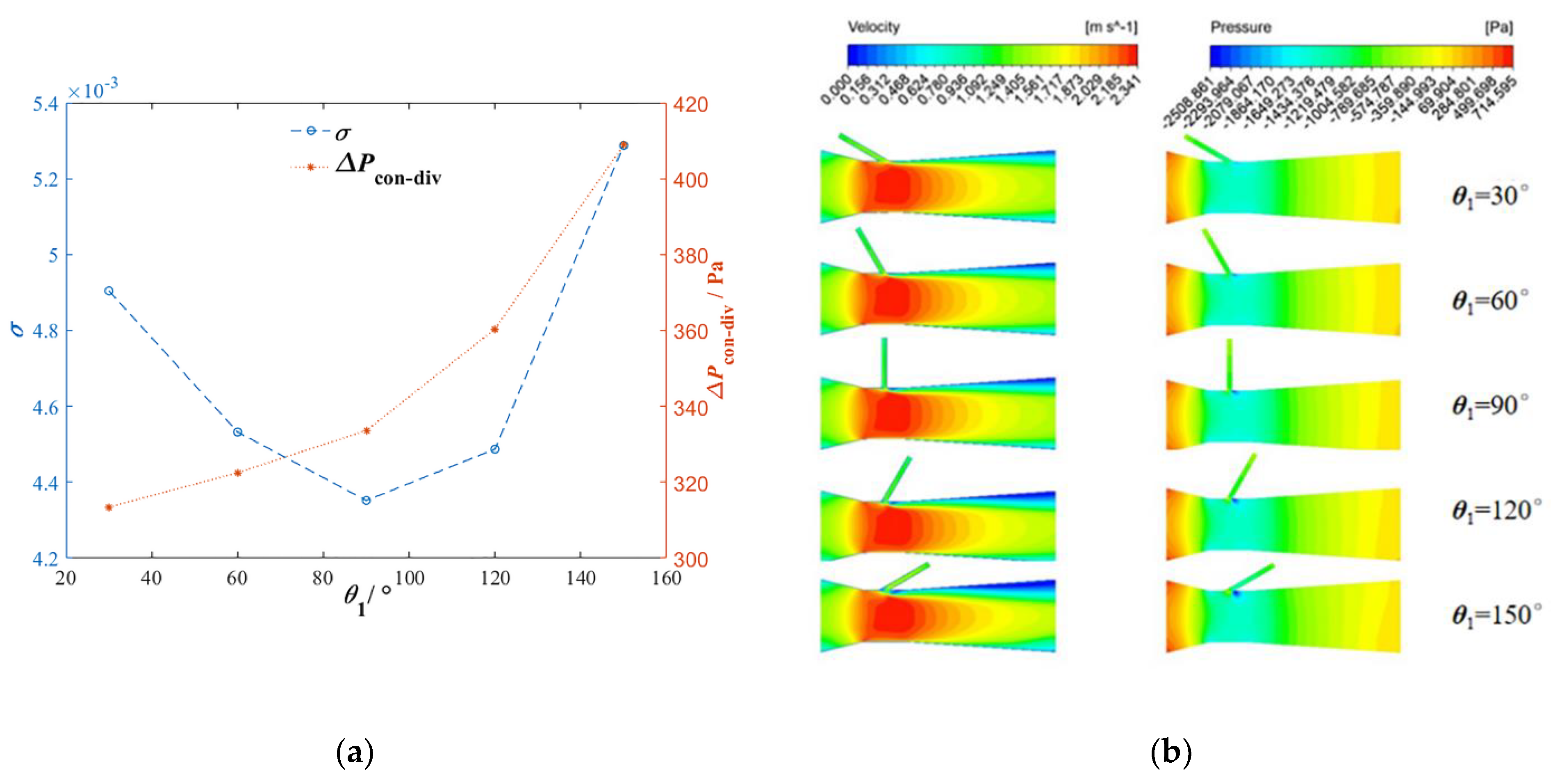
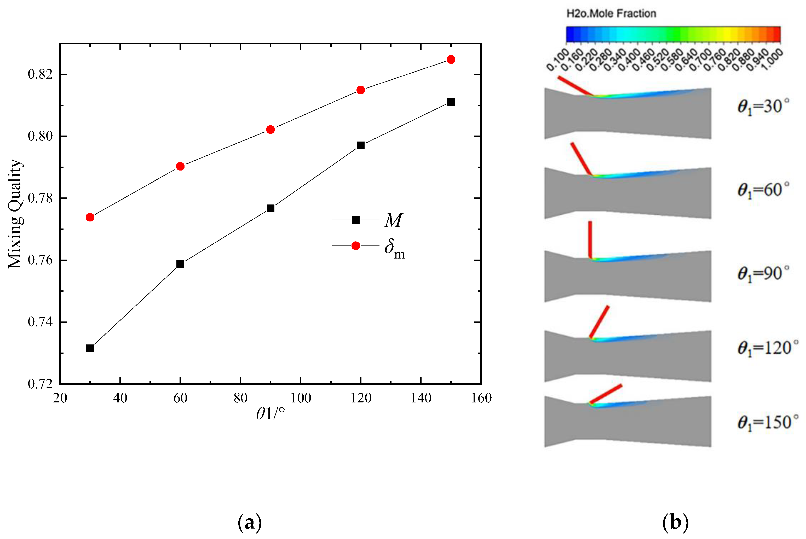
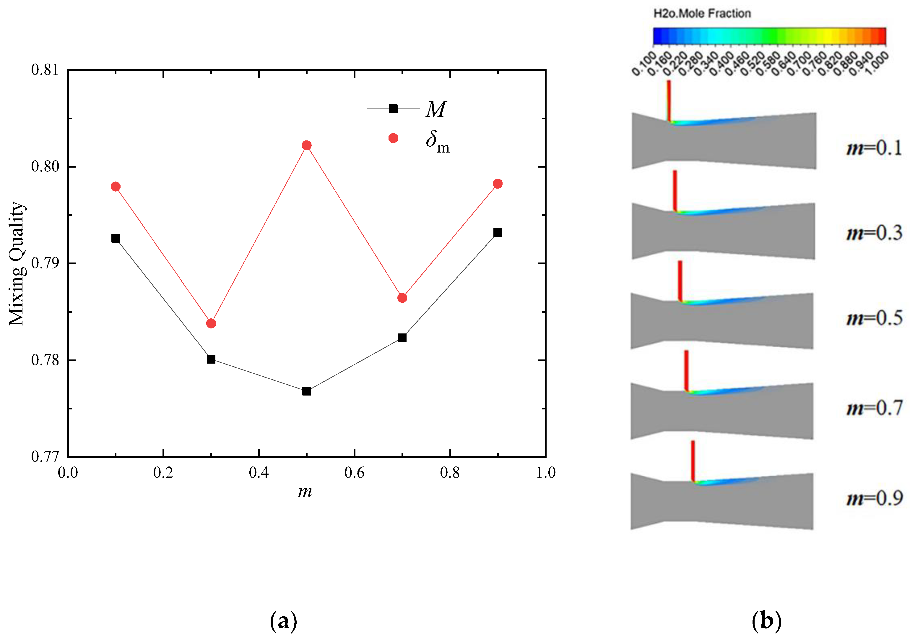
Subsequently, the flow and mixing characteristics in VTM are simulated based on the optimized VT, where the structural parameters’ pore-throat diameter ratio γ₂ (=d_jet/d), jetting angle (θ₁), jetting position ratio m (=l_jet-con/l_thr) and the number of jetting N, and the operating conditions, including the passive suction and active injection, are discussed, where Re is only changed in the operation of passive suction, and R (=v_jet/v_con) is only changed in the active injection operation. These structural parameters in this step are shown in

Table 6. Structural parameters and operating conditions on the flow and mixing simulation in VTM.

ljet, mm	γ2	θ1, °	m	N	Re	R
22.86	0.1	30	0.1	1	13,105	0.5
	0.3	60	0.3	2	34,947	1.0
	0.4	90	0.5	3	56,788	1.5
	0.5	120	0.7	4	78,630	2.0
	0.7	150	0.9	5	100,471	2.5
					122,313	3.0
					144,154	3.5
						4.0

. The operating conditions with passive suction are given in

Table 7. The operating conditions in passive suction of VTM.

Operation	vcon, m/s	Pjet, Pa	Pdiv, Pa
Passive suction	1.106	0	0
	0.415
	1.106
	1.797
	2.488
	3.179
	3.870
	4.561
	0.415

, and the operating conditions with active injection are given in

Table 8. The operating conditions in active injection of VTM.

Operation	vcon, m/s	vjet, m/s	Pdiv, Pa
Active injection	1.106	0.553	0
		1.106
		1.659
		2.212
		2.765
		3.318
		3.871
		4.424

. In the optimization work of VT and VTM, the total number of simulation cases is 70.

2.7. Evaluation of the Flow and Mixing Quality in VT and VTM

In the evaluation of flow in the VT and VTM, variables including the pressure at the throat P_thr, the pressure drop coefficient (λ) and the vacuum transfer coefficient (T) are commonly used. The suction capacity of VTM is directly affected by P_thr, and the suction capacity increases with P_thr. The pressure drop coefficient (λ) can be used to evaluate the energy consumption, which is calculated using Equation (8).

$$\lambda =\frac{\Delta P_{\mathrm{con}-\mathrm{div}}/\rho }{v_{\mathrm{div}}^2/2}$$

(8)

Generally, the energy consumption in the VT is used to conquer the pressure drop between the convergent and divergent regions. To quantify the pressure drop, a dimensionless number lambda is defined as the pressure drop divided by the kinetic energy of the fluid. It is a great convenience to use lambda to characterize the pressure drop even under a different structure of the VT, and that is why lambda can also be named as the energy consumption coefficient. In this work, the fluid material is water with low viscosity, and it can be regarded as an ideal fluid in the case of a rather large Reynolds number; therefore, the energy consumption generated by viscous dissipation is neglected. The vacuum transfer coefficient T is the ratio of vacuum degree to ΔP_con-div, and the larger the value of T, the better the performance of the Venturi tube. The value of T can be calculated using Equation (9).

$$T=\frac{-P_{\mathrm{thr}}}{\Delta P_{\mathrm{con}-\mathrm{div}}}$$

(9)

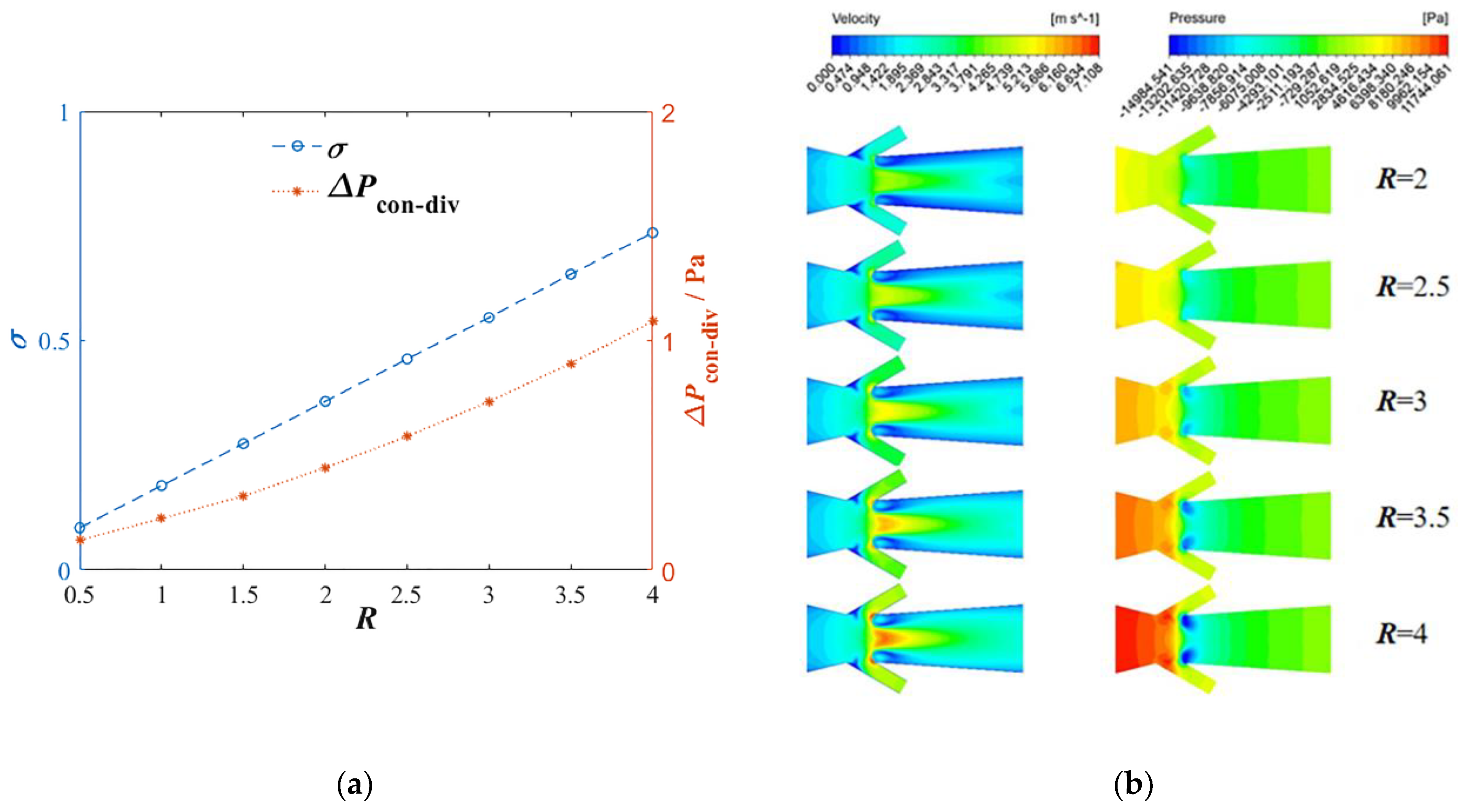
When evaluating the flow and mixing in the VTM, ΔP_con-div, ejecting ratio (σ) and mixing quality (M) are usually used, in which ΔP_con-div can be used to evaluate the energy consumption, and ejecting ratio σ can be used to evaluate the suction capacity, calculated using Equation (10).

$$\sigma =\frac{Q_{\mathrm{e}}}{Q_{\mathrm{c}}}$$

(10)

where Q_e is the volume flow rate of the motive flow, and Q_c is the volume flow rate of the jetting flow.

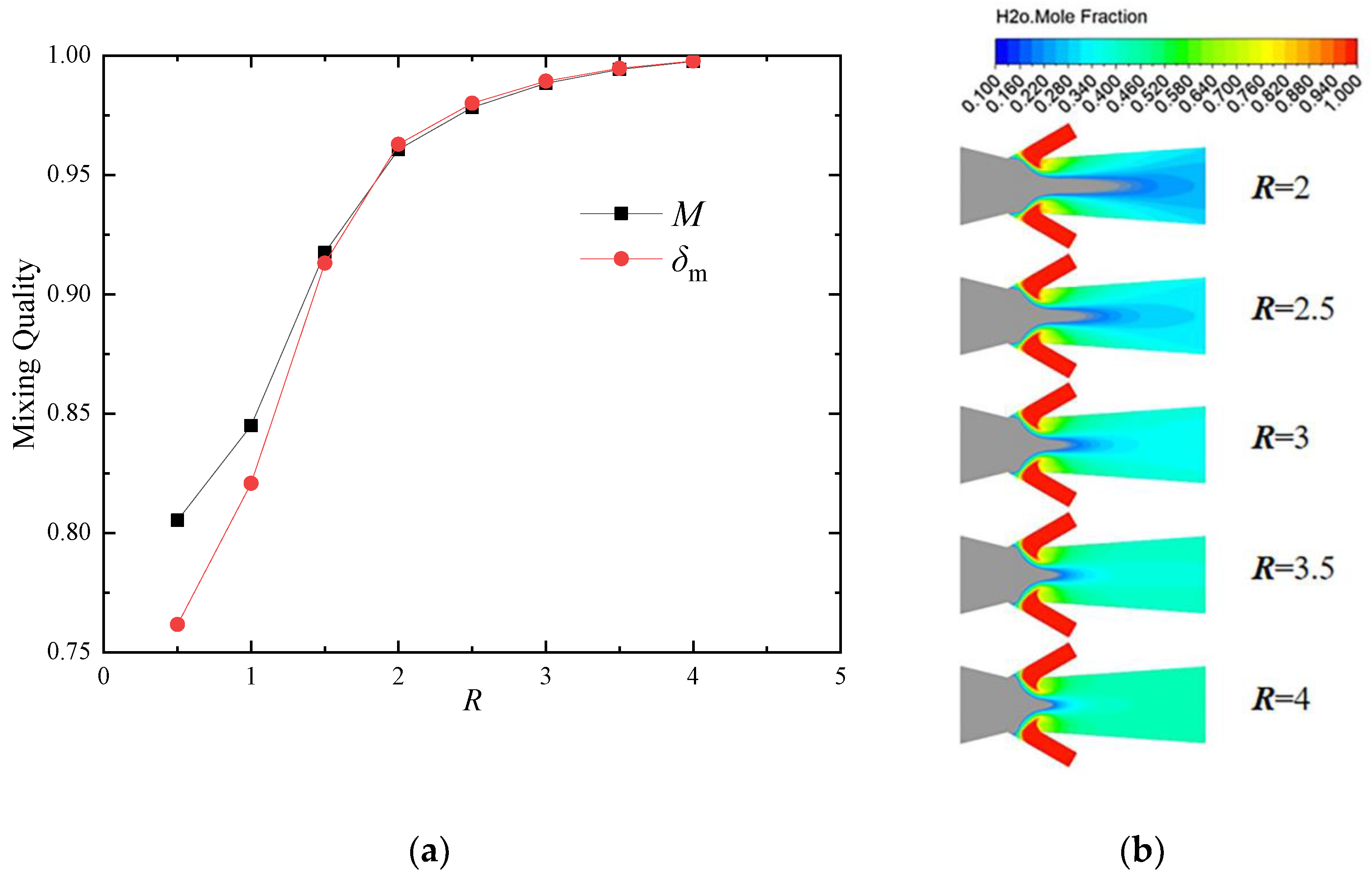
Because the main application of VTM is mixing, the mixing quality of VTM should be considered, which can be characterized by the variable M [24], calculated using Equation (11).

$$M=1-\sqrt{\frac{1}{n}{\displaystyle \sum }_{\mathrm{j}=1}^n\frac{{(k_{\mathrm{j}}-k_0)}^2}{k_0\left(1-k_0\right)}}$$

(11)

where n is the number of sampling points on the concerned plane (for example, the divergent outlet), k_j is the mole fraction of species at the sampling point j, and k₀ is the species average mole fraction on the plane of the divergent outlet. Apparently, the mixing quality M is between 0 and 1, where there is complete mixing if M = 1 and non-mixing if M = 0. Meanwhile, the secondary index δ_m [25] is used to evaluate mixing quality, calculated using Equation (12).

$${\delta }_{\mathrm{m}}=1-\frac{{\sigma }_b}{{\sigma }_{\max }}$$

(12)

where σ_b is the standard deviation of the liquid volumetric flow, which can be calculated using the following expression.

$${\sigma }_{\mathrm{b}}^2=\frac{{\displaystyle \int {(\varphi -{\overline{\varphi }}_{\mathrm{b}})}^2{u}_{x}dydz}}{{\displaystyle \int u_{x}dydz}}$$

(13)

where the u_x is the velocity component in the x direction, and $\stackrel{-}{\varphi }$ is the bulk mass fraction evaluated as the following formula.

$${\overline{\varphi }}_{\mathrm{b}}=\frac{{\displaystyle \int \varphi u_{x}dydz}}{{\displaystyle \int u_{x}dydz}}$$

(14)

The maximum value of σ_b is σ_max, which can be calculated using Equation (15).

$${\sigma }_{\max }=\sqrt{{\overline{\varphi }}_{\mathrm{b}}(1-{\overline{\varphi }}_{\mathrm{b}})}$$

(15)

3. Results and Discussion

3.1. The Results of the Mesh Sensitivity Analysis

3.1.1. Mesh Sensitivity of Venturi Tube

Velocity and pressure distributions along the central axis of VT are shown in Figure 3. It can be observed that the variations of both velocity and pressure along the central axis under five meshing schemes are almost the same. When the number of grid cells reaches 0.13 million, the differences of pressure and velocity distributions between the meshing schemes are indistinct. For the velocity distribution, the largest relative deviation of the result of grid number 0.13 million from that of 0.58 million is within 1.2%, and this deviation is within 0.003% for the pressure. Therefore, the meshing scheme with grid cell number 0.13 million will be adopted in the optimization of VT structure.

3.1.2. Mesh Sensitivity of Cross-Flow

The comparison of velocity distribution along the z-direction is shown in Figure 4, in which the four figures show the velocity distribution on four lines with different x/d_jet. It can be observed that the differences of velocity distribution become obvious with the increase of x/d_jet. When the number of grid cells is 2.61 million, the deviation of velocity from that of grid cell number 8.5 million can be as small as 2%, indicating that the meshing scheme with grid cell number 2.61 million can be acceptable in the prediction of cross-flow in flow characteristics in the VTM.

According to the above analysis of mesh sensitivity, in the numerical simulation of VT and VTM, the meshing scheme will be carried out as follows: in the optimization of the VT configuration (Section 3.1), the grid size will be between 1.18 mm and 2.87 mm, resulting in a total grid number of 0.13 million; in the section of VTM with cross-flow (Section 3.2), there will be refined mesh near the jetting tube, where the minimum size of the grid can be as small as 0.173 mm, which results in a total grid number of 2.16 million. The meshing results of VT and VTM are shown, respectively, in Figure 5a,b.

3.2. The Results of Turbulence Model Selection

3.2.1. Turbulence Model in the Simulation of Venturi Tube

The relationship between pressure drops and Re is shown in Figure 6. It can be clearly seen in Figure 6 that the variation tendency of pressure drops with the Reynolds number is generally the same as that of the theoretical value and experimental results. The simulated results are generally in good agreement with the literature data. The simulated pressure drop is larger than the theoretical value in Figure 6b, which is because the theoretical calculation method considers energy loss caused by local resistance only, while other energy loss such as viscous resistance is ignored.

ΔP_con-div is a crucial index for evaluating the mixing energy consumption of VTM, and consistency between the simulated and experimental results is desired. In Figure 6b, the average relative error, between simulated results and experimental data, from Realizable $k$-$\epsilon$ model is 8.768%, while the relative errors from Standard $k$-$\epsilon$ and RNG $k$-$\epsilon$ are 11.459% and 9.705%, respectively. Apparently, the prediction of ΔP_con-div by Realizable $k$-$\epsilon$ model is more desirable.

3.2.2. Turbulence Model in the Simulation of Cross-Flow

The simulated velocity distributions with various turbulence models along the z-direction in the cross-flow are shown in Figure 7, in which the simulated results are compared with the experimental results of Sherif [22] and the simulated results from Yuan based on the LES method [26].

On the line x/d_jet = 0, the results by RANS method are generally in good agreement with the experimental and LES method results. With the increase of x/d_jet, the difference of the simulated results between RANS and LES methods and the experimental results becomes obvious. On the line x/d_jet = 3.67 (in the black dashed frame), the relative errors between simulated results and experimental data are given in

Table 9. Relative errors (%) between the simulated and experimental results on the line x/d_jet = 3.67.

z/djet	LES	$\mathbf{Realizable} \mathit{k}$$-\mathit{\epsilon }$	$\mathbf{RNG} \mathit{k}$$-\mathit{\epsilon }$	$\mathbf{Standard} \mathit{k}$$-\mathit{\epsilon }$
5.10	7.37	6.99	14.99	9.24
4.58	1.88	10.39	17.91	15.73
4.16	5.51	3.32	10.39	8.10
3.73	10.75	4.78	19.26	17.02
3.24	54.86	29.84	134.08	50.03
2.74	43.51	51.30	101.15	65.44
2.23	30.40	54.29	57.29	58.96
1.82	13.87	36.15	16.05	32.73
Average	21.02	24.63	46.39	32.16

.

As can be seen in Table 5, the maximum and minimum relative errors for LES are 54.86% and 1.88%; for the Realizable $k$-$\epsilon$ model, they are 54.29% and 3.32%; for the RNG $k$-$\epsilon$ model, they are 134.08% and 10.39%; and for Standard $k$-$\epsilon ,$ they are 65.44% and 8.10%. It is clearly revealed that LES has the greatest prediction accuracy, followed by the Realizable $k$-$\epsilon$ model, with a small gap between these two models in prediction accuracy. Therefore, the Realizable $k$-$\epsilon$ model will be used to solve the turbulence in the flow of VTM.

3.3. Optimization of VT Configuration

As the primary part of VTM, the performance of the VT in the fluid flow is of vital importance. In this section, we will discuss the effects of structural parameters on the hydrodynamics of the VT, as the basic condition for the following optimization of VTM. Those structural parameters include the convergent ratio γ₁, length-diameter ratio of throat δ, convergent angle α and divergent angle β, whose physical meanings and values can also be found in Figure 1 and Table 6, respectively.

Figure 8a shows the change of P_thr and λ with the increase in γ₁. As can be seen, there is an obvious change of P_thr and λ, where P_thr decreases from −7692.47 Pa to −604.49 Pa and λ decreases from 3.65 to 0.26. The length-diameter ratio of throat δ has a weak effect on P_thr and λ, as shown in Figure 8c, with a narrow range from −2999.83 Pa to −2933.18 Pa and 1.15 to 1.37, respectively. These results indicate that γ₁ can affect the fluid flow in the VT more than δ, which can also be approved by the velocity and pressure distributions in VT, as shown in Figure 8b,d. The variations of velocity and pressure distributions are distinct with the increase in γ₁, while those are relative steady state with the increase in δ. This is because the variation of γ₁ changes both the local resistance and flow turbulence degree in the throat region, while δ only changes the distance of flow development in a relatively small range.

As for α and β, inverse effects are shown on the suction capacity and energy consumption, where α is positive and β is negative, as shown in Figure 8e,g. That is because α changes the degree of sudden contraction at the convergent region, and β changes the degree of sudden enlargement at the divergent region. With the increase in α, which provides shorter flowing distance for the fluid contraction into the throat, the larger velocity gradient along the axial direction from the convergent inlet to the throat caused by it, as shown in Figure 8f. Such a quick flow contraction consumes more energy to be achieved, as shown in Figure 8f, where the pressure drop between the convergent inlet and the divergent outlet is obvious. As for β, its increase can reduce energy consumption when the fluid flows through the divergent region, which presents as the decrease in pressure drop. However, when β is as large as 18°, there will be a reverse flow near the wall at the divergent outlet, which it is not desirable for the operation of VT and VTM. Therefore, in the designs of VT and VTM, β cannot be increased arbitrarily.

In Section 2.7, we introduced a parameter T to evaluate the performance of the VT, which is defined as the suction capacity divided by the energy consumption. As can be seen in Figure 9, there is a maximum value of T in the range γ₁∈ [0.5, 0.833], δ∈ [0.6, 1.4], α∈ [8°, 40°] and β∈ [6°, 18°], which is roughly between 3.26 and 5.19. Therefore, γ₁ = 0.714, δ = 0.8, α = 28° and β = 8° are the optimized structural parameters of VT, which will be used in the optimization of VTM in the following section.

3.4. The Flow and Mixing Characteristics in VTM

Based on the optimization of VT in the last section, where the configuration of VT with low energy consumption and desirable suction capacity is proposed. In this section, the effect of structural and operational parameters on the flow and mixing in VTM will be discussed, including the pore-throat diameter ratio γ₂, jetting angle θ₁, jetting position ratio m, jetting tube number N and the operating conditions (passive suction and active injection). It should be noted that the operation of VTM is passive suction when the effect of the above structural parameters on flow and mixing in VTM are discussed.

3.4.1. The Effects of Pore-Throat Diameter Ratio on Flow and Mixing in VTM

The pore-throat diameter ratio γ₂ is defined as d_jet divided by l_jet, and five values of γ₂ will be discussed in the range from 0.1 to 0.7 by changing the diameter of jetting tube d_jet.

Figure 10a shows the effects of γ₂ on the ΔP_con-div and σ, whose definitions and physical meanings were introduced in Section 2.7. It can be seen that both of them increase with γ₂ when γ₂ increases from 0.1 to 0.7, which indicates that the suction capacity and energy consumption increase simultaneously with the increase of γ₂. As for the increase in suction capacity, the decrease in friction and local resistance can explain it. With the increase in γ₂, d_jet increases, and the increase in d_jet is positive on the decrease in friction between wall and flow. Meanwhile, the local flow resistance near the juncture between the jetting tube and the throat is reduced. Therefore, it is easier for more fluid to be sucked into the throat through the jetting tube. The increase in suction capacity with γ₂ increasing is also presented by the velocity distribution in the VTM. There are high and low flowing resistance areas, which respectively distribute at the top and bottom of the throat region due to the high difference of velocity between the motive flow and the jetting flow. The motive flow tends to flow through the area with low flow resistance. The resistance increases with more fluid being sucked into the throat region, thus more motive flow tends to flow through the low resistance area; as a result, the velocity of motive flow at the bottom of the throat region increases, as shown in Figure 10b. Meanwhile, the motive flow can transfer more energy to the jetting flow, which results in the increase in pressure drop between the convergent inlet and divergent outlet, as shown in Figure 10b, and it is also the reason why the energy consumption increases with the increase of γ₂.

With the increase in γ₂, the value of mixing quality M shows an increases-decreases trend, with a maximum value M_max = 0.795 when γ₂ is 0.3, as shown in Figure 11a. According to the effect of γ₂ on suction capacity, with the increase in γ₂, the volume flow rate of the jetting flow increases, then the total kinetic energy of the jetting flow increases, which promotes the penetrating depth of the jetting flow into the motive flow, as shown in Figure 11b, where the penetration of the jetting flow has a positive effect on the mixing between two streams. Meanwhile, the velocity gradient along the radial direction of the area where the concentration of the jetting flow is relatively high is not significant, as shown in Figure 10b. It reduces the friction and entrainment effect between two streams; thus, the mass and momentum transfer between the two streams is inappreciable, and therefore it increases the requirement of flow distance to achieve the same mixing quality, as shown in Figure 11b. Hence, in a certain range of γ₂, increasing γ₂ can intensify the mixing by promoting the penetration of the jetting flow. However, when exceeding this range, a negative effect on the mixing caused by the decrease in the friction and entrainment effect between the two streams will be dominant. That is why the variation of M presents the increases-decreases trend with the increase in γ₂. Therefore, in this work, for the purpose of desirable mixing, γ₂ = 0.3 is an appropriate value of jetting tube size in the VTM. As for δ_m, it is incalculable due to the countercurrent; therefore, the comparison between M and δ_m is not discussed.

3.4.2. The Effects of Jetting Angle on Flow and Mixing in VTM

Jetting angle θ₁ can change the impinging direction between the jetting flow and the motive flow, thus affecting the flow in VTM. In this section, five jetting angles will be discussed, with a range from 30° to 150°, where it can be a concurrent flow between the motive and jetting flows when θ₁ is below 90° and a counter flow when θ₁ is larger than 90°.

With the increase in θ₁, ΔP_con-div shows a monotonous increase, while the σ presents a decreases-increases change, as shown in Figure 12a. As for the change of ΔP_con-div, it results from the increase of flow resistance when the interaction between motive flow and jetting flow varies from concurrent to countercurrent, which the energy consumption is increasing. The result of more energy consumption is the increase in the pressure drop between convergent inlet and divergent outlet, as shown in Figure 12b. Meanwhile, with the increase in θ₁, a low-pressure area around the jetting tube is generated by the intensified impingement between the jetting flow and the motive flow, and the low velocity area extends along the downstream from the jetting flow, as shown in Figure 12b.

As for the change of ejecting ratio σ, the variation ranges only from 0.00435 to 0.00529, which indicates that promoting suction capacity by changing θ₁ is not as significant as that by changing γ₂. This is because that with the increase in the inclination degree of the jetting tube, the width of the juncture between the jetting tube and throat increases, which can reduce local flow resistance. It is also the reason why the suction capacity is the lowest under θ₁ = 90°. However, the effect of θ₁ on the suction capacity is limited and is not as efficient as increasing γ₂.

To a certain extent, when the motive flow and jetting flow are countercurrent, the VTM can be regarded as an impinging jetting flow mixer. Therefore, the mixing quality increases with the increase in jetting angle θ₁, as shown in Figure 13a, where M and δ_m increase simultaneously. As a result, the flow developing distance achieving the same mixing quality of the two streams also decreases with the increase in θ₁. Figure 13b shows this phenomenon, where with an increase in θ₁, the axial length of the high concentration area of the jetting flow is shortened by 39% compared to that in the case θ₁ = 30°. Therefore, θ₁ = 150° regarded as a desired value for jetting angle in VTM in terms of mixing quality.

3.4.3. The Effects of Jetting Position on Flow and Mixing in VTM

To describe the jetting position, the parameter m (=l_jet-con/l_thr) is used, which represents the distance from the beginning of jetting to the end of the throat normalized by the length of the throat, and the value of m ranges from 0.1 to 0.9 in this work.

Figure 14 shows the effect of the jetting position on the flow in VTM. With the increase in m, which means that the jetting tube is approaching the end of the throat, the ejection ratio σ decreases at first and then keeps nearly constant, while ΔP_con-div shows a decreases-increases trend. From the variation range of σ, it can be seen that m slightly affects the suction capacity of VTM, and the change in ΔP_con-div is similar to that of σ, which are both less than 10%. This is because there is no variation of the contact area between the jetting flow and jetting tube wall and the width of the juncture between the jetting tube and throat when m increases; thus, the friction and local resistance of the jetting flow are constant. Meanwhile, the variations of ΔP_con-div and σ are only caused by the heterogeneous distribution of P_thr in the throat region, while the difference in P_thr is imperceptible. The weak effect of m on the flow in VTM can also be approved by similar velocity and pressure distributions with various m in VTM.

In terms of mixing, the position of the jetting tube hardly affects the mixing quality between these two streams, where the difference between M_max and M_min is only 0.016 when the value of m ranges from 0.1 to 0.9, as shown in Figure 15a. This is because the variation in m only changes the position where the two streams begin to mix in the throat region, and the length of the throat is not long enough to significantly affect the mixing quality. However, when the jetting tube is located at the very center of the throat, the value of M_min is realized at m = 0.5, which means the mixing quality can be relatively slightly worse. Therefore, a longer distance between the jetting tube and the center of the throat is beneficial to the mixing quality. When the position of the jetting tube is closer to the convergent region, the two streams have a longer distance for the development of mixing. Meanwhile, as can be seen in Figure 14a, the suction capacity is better as well. Therefore, for the mixing quality, m = 0.1 is regarded as desirable for the jetting position in VTM. However, the maximum value of secondary index δ_m is realized at m = 0.5, and it is slightly larger than the value of δ_m when m = 0.1.

3.4.4. The Effects of the Jetting Stream Number on the Flow and Mixing in VTM

In VTM, two or more jetting streams are also a common operation. Therefore, in this section, the effects of the jetting stream number on the flow and mixing will be discussed, from one stream to five streams, where the jetting tube(s) are evenly distributed around the throat. The distribution of jetting streams is shown in Figure 16c.

Apparently, the suction capacity of VTM increases greatly and linearly with the increase in N in a passive way, while the energy loss increases simultaneously, as shown in Figure 16a. For the suction capacity, it can be explained that the variation of N only changes the number of the jetting inlet with the same boundary condition (for example, the ambient pressure at the entrance of the jetting tube), and the increase in suction capacity is directly proportional to the number of jetting tubes. With more fluid being sucked into the VTM, more kinetic energy of the motive flow is consumed to promote the jetting flow rate; it is also the reason why ΔP_con-div increases with the increase of jetting number N. According to velocity and pressure distributions in VTM, only the number of low velocity and pressure areas changes with the variation of N, where the low velocity and pressure areas are caused by the jetting flow and distributed along the downstream near the wall.

In terms of mixing quality, the value of M generally increases with the number of jetting tubes, as shown in Figure 17a. By comparing the values of M when N increases from 4 to 5, the value of M shows no advantage with an increase in N. Along the circumference of the throat, the mixing quality is better with an increase in N. When N is up to 4, the mixing performance of VTM achieves stability; then, by increasing N, it has a weak effect on mixing quality. Therefore, N = 4 can be an optimized value for present VTM. At the same time, the maximum value of δ_m is realized at N = 4, which represents that the mixing quality evaluated by σ_b of VTM with four jetting tubes is relatively better.

To quantitatively reveal the effect of structural parameters on the mixing quality, according to the work of Sobenko et al. [27], an empirical formula for M is obtained as follows:

$$M=1.05{\gamma }_2^{-0.012}{\theta }_1^{-0.084}{m}^{0.005}{N}^{0.04} (R^2=0.95)$$

(16)

This formula is applicative when Re is around 3.5 × 10⁴ to 1.0 × 10⁵.

3.4.5. The Effects of Motive Flow Reynolds Number on the Flow and Mixing in VTM

In this work, we define the passive suction as the jetting flow ejecting into the throat only due to the pressure difference between the throat region and jetting tube entrance, where the energy for the flow and mixing is only from the kinetic energy of the motive flow without any extra energy input (Figure 18). Therefore, the variation in this pressure drop of VTM is governed by the change of motive flow velocity (v_con). In this section, the effects of Reynolds number Re (defined in Equation (7)) of motive flow on flow and mixing will be discussed, with seven values ranging from Re = 13,105 to Re = 144,154.

It can be clearly seen that with an increase in Re, the suction capacity of VTM increases due to the change in pressure in the throat region, which can be explained by the Bernoulli equation, where there is energy transformation from kinetic energy to hydrostatic pressure. As a result, the change in pressure is significant with the increase in flow velocity in VTM, and this variation is proportional to the Reynolds number squared (Re²). In terms of ejecting ratio σ, it only increases from 0.107 to 0.113, even if ΔP_con-div increases from 205 Pa to the level of 10⁴ Pa. This indicates that it is not a cost-effective way of promoting suction capacity by increasing Re under a passive suction operation. In addition, with an increase in Re, the distribution of velocity and pressure loses its uniformity, as shown in Figure 18b, which is caused by the intensified interaction between the jetting flow and the motive flow due to the increasing velocity difference between these two streams. It is negative for mixing with such a velocity difference between the jetting flow and motive flow, because under a certain flow developing distance, a high-velocity motive flow will shorten the contact time between these two streams. As a result, the variation of mixing quality M and δ_m can even be inverse to the increase of motive flow Reynolds number, as shown in Figure 19a. Moreover, the value of δ_m is slightly lower than the value of M.

3.4.6. The Effects of Velocity Ratio between Motive and Jetting Flows on Flow and Mixing in VTM under Active Injection

In addition to passive jetting, active injection is also a common operation in VTM. In this situation, extra energy needs to be inputted to ensure there is a controllable jetting flow rate even when the flow rate of motive flow is changed. In this section, the effect of velocity ratio R (=v_jet/v_con) between the jetting flow and motive flow, with eight values from 0.5 to 4, on the mixing in VTM will be discussed by changing the active jetting velocity v_jet.

Apparently, with the increase in velocity ratio R, ΔP_con-div and σ both increase, as shown in Figure 20a. Meanwhile, comparing velocity distribution in the throat under active injection with that under passive suction, the high velocity area in VTM is reduced, as shown in Figure 18b and Figure 20b, and there is only a relatively small high velocity area near the jetting tube. When the fluid flows into the divergent region, except for some areas with large velocity gradients such as near the wall, the velocity in other areas is basically uniform. In addition, with an increase in R, the high velocity gradient area decreases, as shown in Figure 20b. This phenomenon is beneficial to the mixing. Moreover, there is a low-pressure area around the high-velocity area, and the fluid in this low-pressure area can be easily sucked into the high-velocity area, which also intensifies the mixing. With an increase in R, the jetting flow with more kinetic energy can penetrate deeper into the motive flow, which promotes energy dissipation during their impingement and therefore intensifies the mixing.

In Figure 21a, with an increase in R, the values of M and δ_m are greatly promoted and even approaches 1 in the case of R = 4, and the values of M and δ_m are virtually the same, which can be also observed from the change in jetting fluid concentration distribution along the motive flow direction, as shown in Figure 21b. Comparing the mixing quality between the active and passive operations of jetting flow indicates that the cost of improving mixing quality comes from the additional energy consumption of the active injection. Meanwhile, with an increase in R, the increasing trend of mixing quality M becomes mild, which indicates that it is more cost-effective to increase mixing quality in a certain range by increasing the velocity ratio R.

4. Conclusions

A Venturi tube mixer is a typical process-intensification device, where fast mixing can be achieved by intensive shearing in its throat region. In this work, in order to discover the flow and mixing characteristics of a Venturi tube mixer and thereby its optimization, a two-step method was used, where we firstly optimized the configuration of the Venturi tube without jetting tube by changing the convergent ratio γ₁, length-diameter ratio of throat δ, convergent angle α and divergent angle β of the Venturi tube. Then, based on the optimized Venturi tube, the effects of pore-throat diameter ratio γ₂, jetting angle θ₁, jetting position ratio m, jetting tube number N and the operation mode of jetting flow on the flow and mixing in the Venturi tube mixer were discussed.

In the description of flow in the Venturi tube and the cross-flow, the Realizable k-ε model is an appropriate choice, with a similar average relative error as the LES model but more efficient.

Among all the structural parameters of the Venturi tube mentioned in this work, the convergent ratio is the most influential factor on the flow and the pressure drop in the Venturi tube, while the effects of length-diameter ratio of the throat is not as much as expected. The effects of convergent angle and divergent angle on the flow and pressure drop in the Venturi tube are opposite. Therefore, an optimized configuration of the Venturi tube is proposed, where above parameters are γ₁ = 0.71, δ = 0.8, α = 28° and β = 8°. After the optimization of VT, the pressure drop coefficient of optimized VT reduces by 61.6%, while the vacuum transfer coefficient improves by 44.1%.

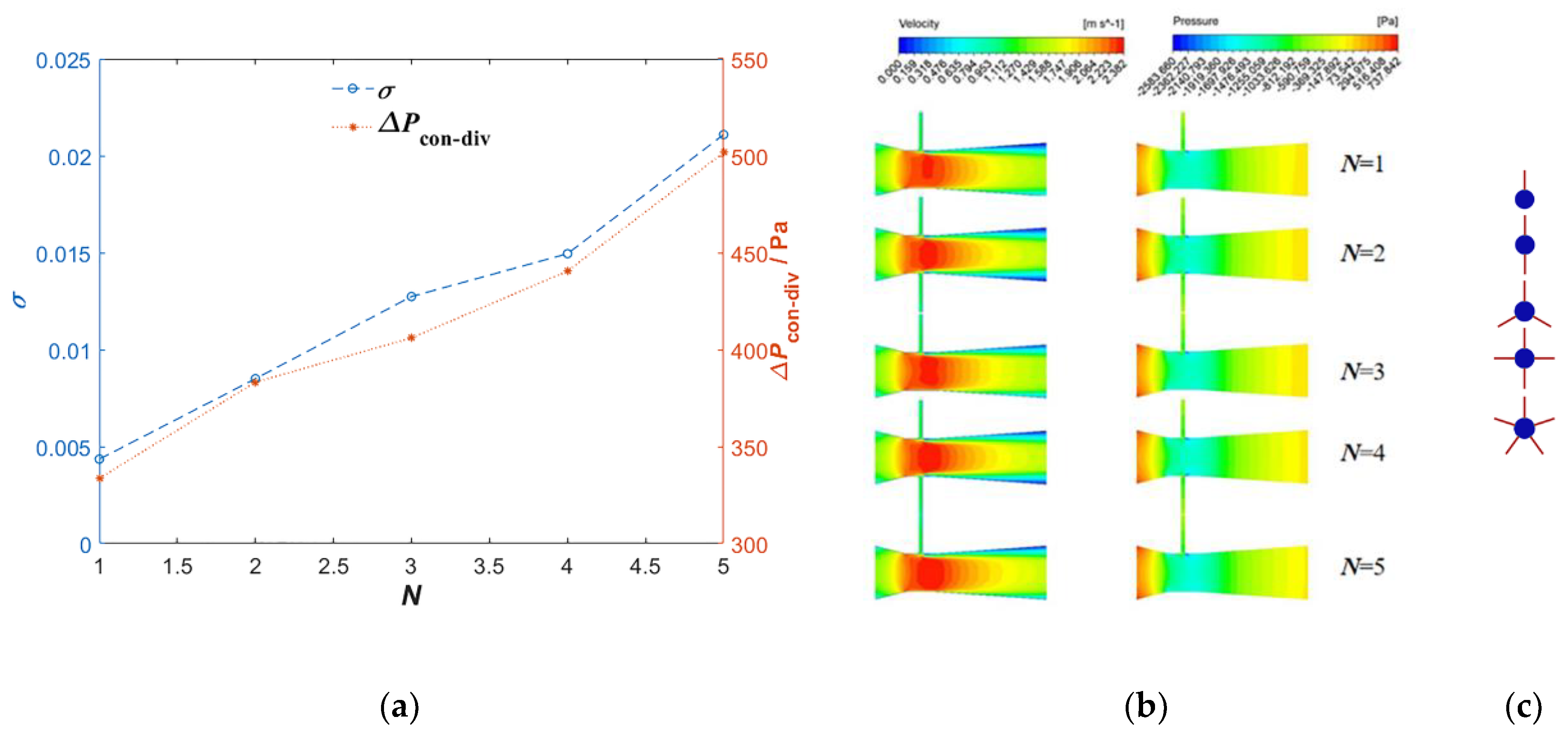
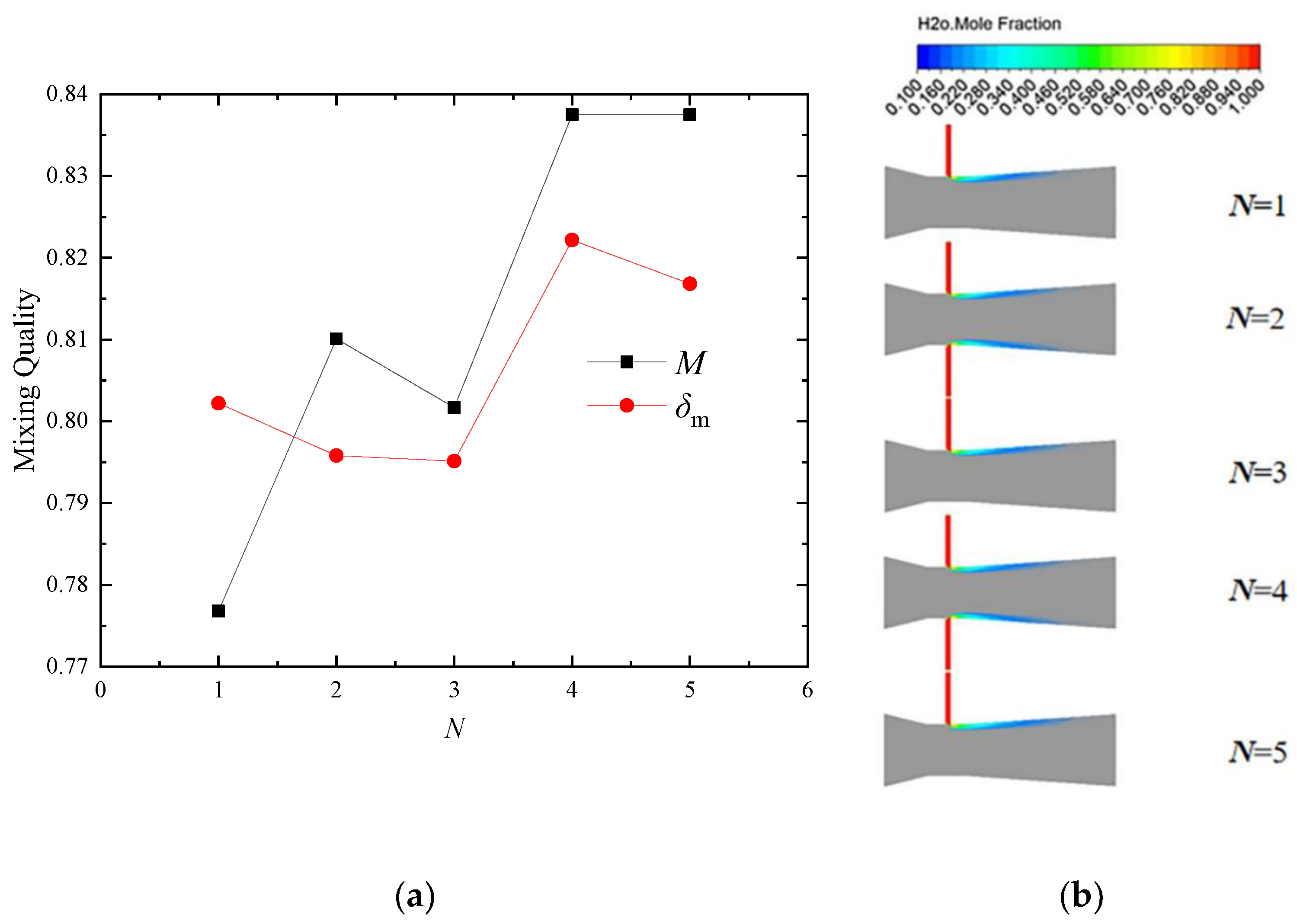
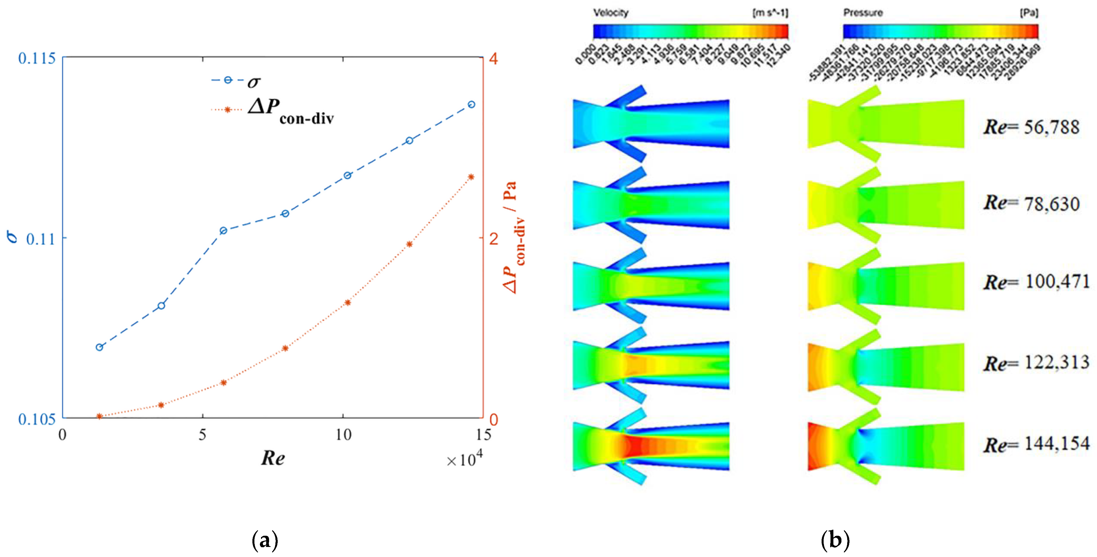
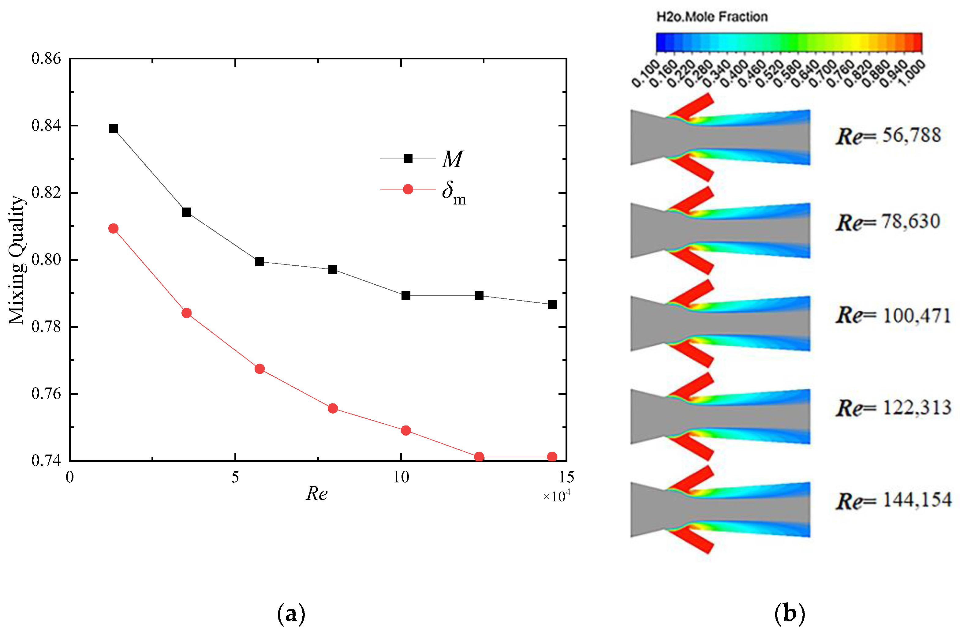
Based on the optimized configuration of the Venturi tube, a jetting tube is introduced to generate cross-flow to realize a Venturi tube mixer. To a reasonable extent, the pore-throat diameter ratio can be beneficial to suction capacity of the Venturi tube mixer. Jetting angle has a significant effect on mixing quality, where a large jetting angle can contribute to the mixing at the cost of energy consumption (pressure drop) in the Venturi tube mixer. The jetting position is a weak factor in affecting the flow and mixing in the Venturi tube mixer, while increasing the number of jetting tubes from single to quadplex can be a positive factor in the mixing quality. Compared with passive suction, active injection can promote mixing more efficiently. As a result, an optimized configuration of Venturi tube mixer (in passive operation) is proposed, where above parameters are γ₂ = 0.3, θ₁ = 150°, m = 0.1 and N = 4. The energy consumption of optimized VTM has decreased by 85.6%, and the mixing quality has increased by 4.8%.

In the chemical industry, VTM plays an important role in some specific processes, for example, the mixing of fluid and fine powders, the generation of micro bubbles to intensify mass transfer, the premixing of ingredients in hydrogenation reaction, etc. According to the research of the mixing characteristics of VTM in this work, help and suggestions in the design of an excellent VTM for industrial applications have been provided.