Article

Deep Belief Network with Swarm Spider Optimization Method for Renewable Energy Power Forecasting

1
Northwest Electric Power Design Institute, Xi’an 710075, China
2
Department of Electrical Engineering, Xi’an University of Technology, Xi’an 710048, China
*
Author to whom correspondence should be addressed.
Processes 2023, 11(4), 1001; https://doi.org/10.3390/pr11041001
Submission received: 22 November 2022 / Revised: 17 December 2022 / Accepted: 23 December 2022 / Published: 26 March 2023

Abstract

:
Renewable energy power prediction plays a crucial role in the development of renewable energy generation, and it also faces a challenging issue because of the uncertainty and complex fluctuation caused by environmental and climatic factors. In recent years, deep learning has been increasingly applied in the time series prediction of new energy, where Deep Belief Networks (DBN) can perform outstandingly for learning of nonlinear features. In this paper, we employed the DBN as the prediction model to forecast wind power and PV power. A novel metaheuristic optimization algorithm, called swarm spider optimization (SSO), was utilized to optimize the parameters of the DBN so as to improve its performance. The SSO is a novel swarm spider behavior based optimization algorithm, and it can be employed for addressing complex optimization and engineering problems. Considering that the prediction performance of the DBN is affected by the number of the nodes in the hidden layer, the SSO is used to optimize this parameter during the training stage of DBN (called SSO-DBN), which can significantly enhance the DBN prediction performance. Two datasets, including wind power and PV power with their influencing factors, were used to evaluate the forecasting performance of the proposed SSO-DBN. We also compared the proposed model with several well-known methods, and the experiment results demonstrate that the proposed prediction model has better stability and higher prediction accuracy in comparison to other methods.

1. Introduction

The electric power industry is an important basic industry of the national economy, and it is the key and leading industry in national economic development strategy. Its development is the need of social progress and the continuous improvement of people’s living standards, and our lives are already inseparable from electricity. In the past, the main generation mode of electricity was thermal power generation from fossil energy, including coal, natural gas and other combustibles. However, the wide application of thermal power will not only lead to a large amount of non-renewable energy consumption, but also discharge many harmful gases in the whole combustion process, causing damage to the natural environment [1]. In order to solve the problems of energy demand and environmental protection, some new clean energy power generations have increased rapidly with the implementation of renewable energy development strategy and the steady progress in the construction of large clean energy bases in the world. In these bases, photovoltaic power generation and wind power generation, as the most typical representatives, have been applied as generating systems by using solar energy and wind energy, owing to the characteristics of being widely distributed and safe to use. On the one hand, solar energy has the advantages of being clean, safe and noiseless, but due to the influence of many factors, it is random, volatile and intermittent [2], which can pose a serious threat to the stability and security of the power grid. On the other hand, wind energy has the characteristics of low pollution and large storage capacity, but it is also intermittent and uncertain, [3] which makes it more difficult to plan and schedule for the grid. All in all, the output powers of solar and wind are instable because of the influence of natural factors, which bring many problems to power grid planning and scheduling of energy management systems, including new energy sources [4] and reliable operation of the power grid. Therefore, it is of great significance to study photovoltaic power and wind power forecasting, and accurate forecasting results are very important for power grid dispatching, energy management and the security and stability of the power system.
In recent years, more and more forecasting approaches have been developed for PV power and wind power, which can be divided into physical-model-based forecasting methods and data-driven methods from the perspective of the mathematical algorithm. The physical approach is based on the principles of wind turbine and solar panel power generation, in which the weather forecast data from numerical weather prediction (NWP), such as wind speed and direction at different heights, normal direct radiation data, horizontal direct radiation data, total radiation data, barometric pressure data, temperature data, and so on, are used to compute the power, combining energy conversion efficiency and system parameters [5,6]. Although the physical-model-based forecasting methods can reflect the internal law, the forecasting results show large deviations in medium- and long-term prediction because the establishment of the model is based on the independence assumption of the local law, and the model parameters are relatively difficult to obtain. Meanwhile, data-drive methods with strong nonlinear fitting ability can make up for the draws of the physical model method, among which the statistical learning and artificial neural network approaches have been extensively applied for the fields of PV power forecasting and wind power forecasting. Statistical learning methods use historical data such as wind, solar, humidity and temperature meters, as well as curve fitting parameter estimation methods, to form input–output mapping models [7,8]. Common statistical methods include time series forecasting methods with high computational speed [9], relatively simple and convenient regression analysis methods [10], grey theory methods that do not require large samples [11], fuzzy theory methods with good robustness [12], spatio-temporal correlation methods that tap deep spatio-temporal features [13], support vector machine (SVM) [14] and other related methods. Time series data can essentially reflect the trend of a particular or certain random variable changing continuously over time, and the core of the time series forecasting problem is to mine this pattern from the data and use it to make estimates of future data [15]. Time series forecasting is widely used in wind and PV power forecasting because of the obvious trend in wind and PV power over time, such as with the Autoregressive Integrated Moving Average model (ARIMA) and the Seasonal ARIMA model (SARIMA) [16,17]. The nonlinear, stochastic nature of wind and PV data poses a great challenge for power forecasting [18,19]. Their historical power and the nonlinear mapping relationship between the time series power data and the influencing factors of power are difficult to capture artificially [20]. As another important data-driven method, artificial neural network (ANN) models with strong nonlinear fitting capabilities can be utilized to forecast PV and wind power, such as with back propagation (BP) [21], radial basis function (RBF) [22], extreme learning machine (ELM) [23], long-short term memory (LSTM) [24,25,26,27], gate recurrent unit (GRU) [28,29,30,31,32], deep belief network (DBN) [33,34] and so on. The BP neural network has strong self-learning ability and complex nonlinear function-fitting ability, but its network initial parameters are obtained by random initialization, resulting in poor generalization ability in prediction cases and an ease for falling into local optimum.
Relative to the aforementioned shallow neural network models, deep neural network (DNN) models have the ability to capture the implied features of nonlinear data so well as to approximate any nonlinear function with deep structure. At present, various DNN model shaves been developed and widely used in the fields of image and audio recognition and clean energy power prediction [32,35]. Recurrent neural networks (RNN), as DNNs, showed prominent performance in time-series forecasting and prediction applications, and the LSTM and NARX, as one of the main efficient RNNs, is suitable for forecasting wind power and PV power [24,25,26,27]. As a LSTM variant, the gated recurrent unit (GRU) network has a simplified configuration that involves fewer training parameters, and it can obtain similar forecasting accuracy to LSTM while involving fewer iterations in several application areas [28]. Thus, the GRU network has been applied for wind power and PV power forecasting [29,30,31,32]. Seq2Seq is generally implemented through the Encoder–Decoder framework. The Encoder and Decoder parts can be any text, speech, image or video data, and the model can be CNN, RNN, LSTM, GRU, BLSTM, etc. Moreover, Seq2Seq is good at exploiting information from long-range global sequences. Therefore, Seq2Seq has also been applied to wind power prediction [36].
DBN is one of the classical deep learning algorithms, which is made up of multiple Restricted Boltzmann Machines (RBM) [37]. Compared with traditional machine learning algorithms, the DBN, with its stronger feature extraction ability, can perform fast analysis of large amounts of data, with powerful data-fitting capability via incorporating deep learning and feature learning. The initial parameters of the network are obtained through layer-by-layer unsupervised pre-training, which effectively solves a series of problems caused by the random initialization of traditional neural network parameters; in addition to having good initial points, the over-fitting and under-fitting problems that often appear in NN models can also be effectively solved through pre-training [38]. In recent years, DBN has been applied in classification, fault diagnosis, data prediction and other fields [34,36,39,40,41]. Considering the advantages of the DBN, it can naturally be applied to the field of clean energy forecasting.
The application of DBN in the field of renewable energy forecasting has been relatively short-lived. In recent years, many scholars have performed a lot of work to employ the DBN in renewable energy power forecasting. Wang used DBN and the k-means algorithm to process meteorological factor data for wind power prediction [42]; Yuan used singular spectrum analysis and optimization algorithms to build a sub-feature set to improve the performance of a DBN model in short-term wind power prediction [43]; Yuba Tao used grey correlation analysis to find the key factors in the time-scale data of wind power generation and used DBN to mine the hidden laws [44]; Wang identified the dynamic characteristics of wind speed by reconstructing the multi-dimensional phase space to facilitate DBN for short-term wind power forecasting [45]; and Wei used wavelet soft thresholding to remove the high-frequency noise signals in the data [46], which ultimately improved the efficiency of the model. An improved DBN was proposed by introducing the Gaussian–Bernoulli restricted Boltzmann machine for wind power forecasting [47], and an adaptive learning step technique was applied to improve the convergence speed. Considering the optimal hyper-parameter in DBN, a particle swarm optimization (PSO) and modified coot optimization algorithm were introduced into the DBN to improve the accuracy of the wind power forecasting [48,49]. All in all, the DBN is a good candidate to be utilized for clean energy power forecasting. However, the hyper-parameter optimization problem is still a key challenge for DBN in prediction fields. The above problem has been significantly changed with the advent of various optimization algorithms, of which metaheuristic optimization algorithms have been widely used in recent years. Various metaheuristic algorithms are local search algorithms that have been developed based on a particular phenomenon: for example, particle swarm algorithms (PSO), genetic algorithms (GA), simulated annealing algorithms (SA), swarm spider optimization algorithm (SSO), etc. SSO is a group intelligent evolutionary algorithm based on the simulation of individual and group collaborative behavior in swarming spiders. Individuals of different sexes have two different evolutionary operators and mimic different collaborative behaviors within the group. The algorithm has good convergence speed and global search capability. To the best of our knowledge, SSO algorithm [50], as an outstanding swarm intelligence optimization method, has been utilized in various applications [51,52], but it has not been used for the optimization problem in DBN. Therefore, the main object of this work was to develop an SSO-optimized DBN model for wind and PV power forecasting.
The power generated from renewable energy sources is significantly influenced by environmental factors, and the forecasting accuracy of the input matrix constructed from a single historical power is not ideal. In this paper, the forecasting accuracy of the model is improved by inputting data containing historical power data, as well as highly correlated influencing factor data. Furthermore, the DBN model has the obvious advantages in renewable energy power forecasting mentioned above, but the prediction potential of the model in renewable energy is significantly influenced by hyper-parameters. In this paper, the SSO algorithm is used to find the optimal number of nodes in the implicit layer of the DBN so that the predictive power of the DBN model can be fully utilized.
The main contributions of this paper are as follows:
  • To the best of our knowledge, this is the first effort to incorporate the SSO into the DBN to optimize its parameters, and thus, the performance of the DBN is further improved;
  • Based on the relevance analysis, the historical power and highly correlated influencing factors are used to construct multidimensional inputs to train the DBN optimized by the SSO method, and a novel hybrid forecasting model is developed for renewable energy prediction;
  • Two datasets, including wind power data and PV power data, are used to verify the prediction performance of the proposed model for renewable energy prediction through comparison experiments under various conditions.
  • The organization of the paper is as follows. Section 2 presents the methodologies, including deep belief network and swarm spider optimization method. Then, Section 3 introduces the proposed forecasting model via the DBF optimized using SSO. Section 4 elaborates on some case studies of the proposed forecasting model based on wind power data and PV power data. Finally, Section 5 concludes this work.

2. Methodology

2.1. Deep Belief Network

DBN has a multilayer neural network structure, and it is a multilayer probabilistic machine learning model. Traditional MLP is faced with the problems of gradient disappearance, the fact of being time-consuming and the large demand for training data; nonetheless, DBN is a practical deep learning method to handle these drawbacks. DBN has an unsupervised learning process and a supervised learning process, where unsupervised learning is accomplished by a network structure with multiple layers of Restricted Boltzmann Machine (RBM) bodies, and supervised learning is performed by a layer of back-propagation networks. Unsupervised learning completes the initialization of the parameters of each layer of the network structure, while supervised learning fine-tunes the initialized parameters globally [53].
A RBM has a visible layer and a hidden layer. The visible and hidden layers are connected in both directions, but the nodes of each layer are not connected to each other. The structure of RBM can be viewed in Figure 1a. During the learning process of RBM, an energy function E ( v , h   |   θ ) should be defined, and a commonly used resolving formula of the energy function is expressed as
E ( v , h | θ ) = i = 1 n j = 1 m ω i j v i h j i = 1 n b i v i j = 1 m c j h j
where v = v 1 , v 2 , , v n T denotes the visible layer, h = h 1 , h 2 , , h m denotes the hidden layer, ω = ω i , j R n × m denotes the weight matrix connecting the two layers and b = b 1 , b 2 , , b n T , c = c 1 , c 2 , , c m T denotes the bias of v , h respectively. θ = ω i j , b i , c j is a parameter set of the RBM.
This structure of the RBM allows the values of the visible and hidden layers to be uncorrelated with each other. Instead of computing each neuron one at a time, the entire layer can be computed in parallel. Then, the probability distribution of the visible and hidden layers is:
p ( v , h   |   θ ) = e E ( v , h | θ ) / Z ( θ )
Z ( θ ) = v h e E ( v , h | θ )
where Z ( θ ) is the normalization constant.
Thus, the probability of a neuron hj being activated in the hidden layer of an RBM is
p h j = 1 v ; θ = f c j + i = 1 n ω i j v i
Since the layers of the RBM are connected in both directions, neurons in the visible layer vi can also be activated by neurons hj in the hidden layer, and its probability can be expressed as
p v i = 1 h ; θ = f b i + j = 1 m ω i j h j
The RBM training process learns the value of the parameter θ to fit the given training data. The non-supervised learning process of the RBM usually uses the Contrastive Divergence (CD) algorithm to update the parameters, and the update rules for each parameter are as follows:
Δ ω = ε E d a t a v i h j E r e c o n v i h j
Δ c = ε E d a t a h j E r e c o n h j
Δ b = ε E d a t a v i E r e c o n v i
where ε is the learning rate for RBM training, Edata is the mathematical expectation over the distribution defined by the training dataset and Erecon is the expectation over the distribution defined by the reconstructed model.
Several unsupervised RBMs and a layer of supervised BPs form a complete DBN, the structure of which is shown in Figure 1b.

2.2. Swarm Spider Optimization Algorithm

The swarm spider optimization (SSO) algorithm seeks to find the optimal target by simulating the social behavior of swarming spiders. In this algorithm, individual spiders live in a constructed high-dimensional spider web. The spiders’ movements, mating and other behaviors constantly change the location of the spiders. The location of the spider represents the value of the independent variable of the objective function, and the weight of the individual spider represents the value of the dependent variable of the objective function [50]. The whole process of the SSO algorithm consists of the following 6 steps.
(1)
Let the spider population be in an n-dimensional search space. In a population of spiders whose total number is N, the number of females is Nf and the number of males is Nm. The equations for Nf and Nm are
N f = F l o o r 0.9 r a n d × 0.25 × N
The spider population consists of a female spider subpopulation F = f 1 , f 2 , , f N f and a male spider subpopulation M = m 1 , m 2 , , m N m .
(2)
The calculation of the weight of each spider is
w i = J ( s i ) w o r s t s b e s t s w o r s t s
where J(si) is the objective function fitness value corresponding to the location of spider i.bests and worsts are defined as follows:
b e s t s = m a x k 1 , 2 , , N J s k
w o r s t s = min k 1 , 2 , , N J s k
(3)
In a common network, the vibration transmitted between spiders is defined as:
V i b i , j = w j e d i , j 2
where di,j is calculated as:
d i , j = s i s j
(4)
Population initialization is defined as follows:
f i , j 0 = p j l o w + r a n d ( 0 , 1 ) p j h i g h p j l o w
where fi,j is the jth parameter at the location of the ith female spider. f i , j 0 denotes the initial set of parameters for the female spider. p j high and p j low denote the upper and lower bounds of the elements of the set of parameters to be optimized.
m k , j 0 = p j l o w + r a n d ( 0 , 1 ) p j h i g h p j l o w
denotes mk,j as the jth parameter at the location of the kth male spider.
(5)
Movement is defined as follows:
f i k + 1 and m i k + 1 denote the position of the spider in the search space.
Based on the cooperative mechanism, the change in position of the female spider is calculated as follows:
f i k + 1 = f i k + α Vibc i s c f i k + β Vibb i s b f i k + δ rand 0.5 with   probability PF f i k α Vibc i s c f i k β Vibb i s b f i k + δ rand 0.5 with   probability 1 PF
where α, β, δ and rand are random constants between zero and one. k is the number of iterations. Sc indicates the individual closest to having the higher quality i. Sb denotes the best individual within population S.
Based on the cooperative mechanism, the change in position of the male spider is calculated as follows:
m i k + 1 = m i k + α Vibf i s f m i k + δ rand 0.5 , if w N f + i >   w N f + m m i k + α h = 1 N m m h k w N f + h h = 1 N m w N f + h m i k , if w N f + i w N f + m
(6)
Mating behavior is defined as follows.
The radius of the mating range is calculated using the formula:
r = j = 1 n p j high p j low 2 n
During mating, each spider determines the probability of impact by means of a roulette wheel:
Ps i = w i j T k w j
A detailed flowchart of the SSO algorithm is shown in Figure 2.

3. Forecasting Model via SSO-DBN

In this section, the workflow of the developed SSO-DNB-based forecasting model is summarized. The main idea of the SSO-DBN is to select the numbers of the optimal hidden node of the DBN using the SSO method. In order to use the proposed model for wind power prediction and PV power prediction, the following procedure is presented.

3.1. Data Collection

Two different datasets are used in this work, i.e., the wind power and PV power prediction problems will be considered.
(1) The wind power dataset was obtained from a wind farm in northwest China in 2022. The temporal resolution of the dataset is 15 min. For the wind power prediction case, the training set is 17,000 data from 0:00 on 1 January 2022 to 13:00 on 28 June 2022, and the test set is 96 data from 13:15 on 28 June 2022 to 13:00 on 29 June 2022. Figure 3 shows the curves of the wind power and each of the four influencing factors (including Maximum Wind Speed (MaWS), Minimum Wind Speed (MiWS), Average Wind Speed (AWS) and Average Outdoor Temperature (AOT)) obtained from NWP over the time period in the test set. From Figure 3, one can observe that the variation trend of the wind power curve is consistent with the wind speed, and it is not similar to the AOT curve. As a result, we can conclude that the wind power is mainly affected by MaWS, MiWS and AWS, and this conclusion can be tested by the following relevance analysis.
(2) The PV dataset was obtained from a PV farm in the Australian Solar Energy Centre in 2016. For the PV power forecasting case, the training data are 19,968 data from 0:00 on 1 August 2016 to 23:45 on 24 February 2017, and the test set is 96 data from 0:00 on 25 February 2017 to 23:45 on 25 February 2017. Figure 4 shows the curves of the PV power and each of the four influencing factors (including Global Horizontal Radiation (GHR), Diffuse Horizontal Radiation (DHR), Weather Temperature Celsius (WTC) and Weather Relative Humidity (WRH)) over the time period from the test set. From Figure 4, we can see that the variation trend of the PV power curve is similar to the GHR, DHR and WTC curves, and it is different from the WRH curve. Therefore, one can know that the PV power is mainly affected by GHR, DHR and WTC, and this conclusion can also be verified by the following relevance analysis.

3.2. Relevance Analysis

The Pearson correlation coefficient requires the analyzed variables to be linear and normally distributed, but wind farm data are nonlinear and does not apply to the Pearson correlation coefficient. Spearman’s coefficient is not only applicable to continuous variables, but also to discrete variables, and can be used to better deal with nonlinear wind power data. Therefore, Spearman’s correlation coefficient was used to analyze the relationship between each factor and the power generated, and to quantitatively identify the factors that show a strong correlation with the power generated.
Spearman’s correlation coefficient (SCC) is a non-parametric measure of the dependence of two variables, and it is widely applicable because it does not take into account whether the variables are linear or not, as well as the overall distribution pattern of the variables and the sample size. Therefore, any pair of two variables can be analyzed for dependence using the SCC, which is calculated using the formula shown below:
ρ s = i = 1 N R i R ¯ S i S ¯ i = 1 N R i R ¯ 2 i = 1 N S i S ¯ 2 = 1 6 i = 1 N d i 2 N N 2 1
where R i and S i are the rank order of the observations after sorting the vectors x, y, respectively; R ¯ and S ¯ are the average rank of the vectors x, y of average rank order; N is the total number of observations; and  d i = R i S i , denotes the difference in rank of observation i between the two variables. ρ s represents the degree of association between two variables; the range of values is 1 , 1 .
As shown in Table 1 and Table 2, the correlation between each influencing factor and power generation in wind power and photovoltaic power was obtained by SCC analysis in this paper. After that, the four influencing factors with stronger correlations were selected as the input quantity of the dataset in this paper, so as to improve the forecasting accuracy of the model. As mentioned above, the influencing factors selected for wind power were MaWS, MiWS, AWS and AOT. The influencing factors selected for PV power mainly included GHR, DHR, WTC and WRH.

3.3. Data Preprocessing

Because the magnitude of the value range of the original data variables varies greatly, the normalization method is utilized to prevent the modeling accuracy from being affected by the numerical dimensional differences:
x = x x m i n x m a x x m i n
where x is the normalized input value, x is the input value of the forecasting model and x m a x and x m i n denote the maximum value and minimum value of the input sequence, respectively.

3.4. The Proposed Model

Combining the DBN and SSO, a novel hybrid model is developed for wind power and PV power forecasting cases in this subsection, in which the SSO is used to optimize the parameters of the DBN iteratively and further improve its prediction accuracy. The detailed procedures can be described as follows.
Step 1. Obtaining the original data, including wind data and PV data. The characteristics of the data are analyzed, and the outliers in the original data are removed. In addition, some missing data in the original dataset should be supplied by some available estimate methods.
Step 2. Relevance analysis. The SCC method presented in 3.2 is used to perform the relevance analysis between the power and other influence factors. According to the results of the relevance analysis, the main features will be determined, and the factors with low relativity for the target parameters will be deleted.
Step 3. Model training. Here we construct the training data according to the results of the relevance analysis in 3.2. The input and output data of the training data for wind power forecasting case and PV power forecasting case are expressed as Formulas (23) and (24), respectively.
T r a i n _ i n _ w i n d ( i ) = P w i M : i 1 , W s i T r a i n _ o u t _ w i n d ( i ) = P w ( i )
where P w ( i ) denotes the wind power value at time i and W s ( i ) denotes the set of influences at moment i, where the influences are selected by the correlation analysis of 3.2. M represents the embedded dimension of the historical power.
T r a i n _ i n _ P V ( i ) = P P V i M : i 1 , P s i T r a i n _ o u t _ P V ( i ) = P P V ( i )
where P P V ( i ) denotes the PV power value at time i and P s ( i ) denotes the set of influences at moment i, where the influences are selected by the correlation analysis of 3.2. M represents the embedded dimension of the historical power.
As shown in Figure 5, by using the training data and setting the initial parameters of the DBN, the DBN model will be trained. Furthermore, the SSO algorithm performs an optimization to search for the optimal number of nodes in the hidden layer of the DBN.
Step 4. Model testing. When the training procedure is finished, the forecasting models will be constructed. The input data of the test data, constructed similarly to the training data in Formulas (25) and (26), are used as the input of the trained model, and the output of the model is the prediction results.
Step 5. Model evaluation. According to the real output of the test data and forecasting results in testing stage, the prediction performance can be evaluated by the following evaluation indicators (including RMSE, MAE, MAPE and MSE), defined as
R M S E = 1 n i = 1 n P p red , i P t e s t , i 2
M A E = 1 n i = 1 n P p r e d , i P t e s t , i
M A P E = 1 n i = 1 n P p r e d , i P t e s t , i P t e s t , i
M S E = 1 n i = 1 n P p r e d , i P t e s t , i 2
where P p r e d , i and p t s e t , i denote the predicted and actual values of power at time i. n is the total number of time points in the whole prediction period.
The overall flowchart of the forecasting model via the SSO-DBN for wind power and PV power is shown in Figure 6.

4. Case Study

In this section, we perform several experiments to verify the performance of the proposed model for wind power prediction and PV power prediction, respectively. In the proposed SSO-DBN method, the initialization settings of SSO are the total number of individuals in the spider population (spidn = 50) and the number of population iterations (in wind power, itern = 60; in photovoltaic power, itern = 100), and the other parameters of DBN are set as follows: numepochs = 1, batchsize = 10, momentum = 0.1, alpha = 0.001. To perform comparative research, we mainly compare the performance of the proposed method with traditional BP, LSTM and DBN methods in the following experiments.

4.1. Wind Power Forecasting

4.1.1. Testing the Prediction Performance under Different Inputs

According the aforementioned discussion in Section 3, we know that the output wind power is affected by many factors, and different factors will show different correlations with the power. Therefore, we first conduct an experiment to investigate the prediction performance of the proposed model under different combinations of the influencing factors in this subsection. The prediction results are shown in Figure 7. One can observe that clear differences exist among the different factors as the inputs of the model. As the same time, we see that the prediction results gradually worsen with the decrease in the number of influencing factors. Furthermore, we can see from Figure 7 that the AOT has a relatively small impact on the output power, which is consistent with the result in 3.2. According to the results in this experiment, we conclude that the combination of the four factors, including MaWS, MiWS, AWS and AOT, should be used as part of the input.

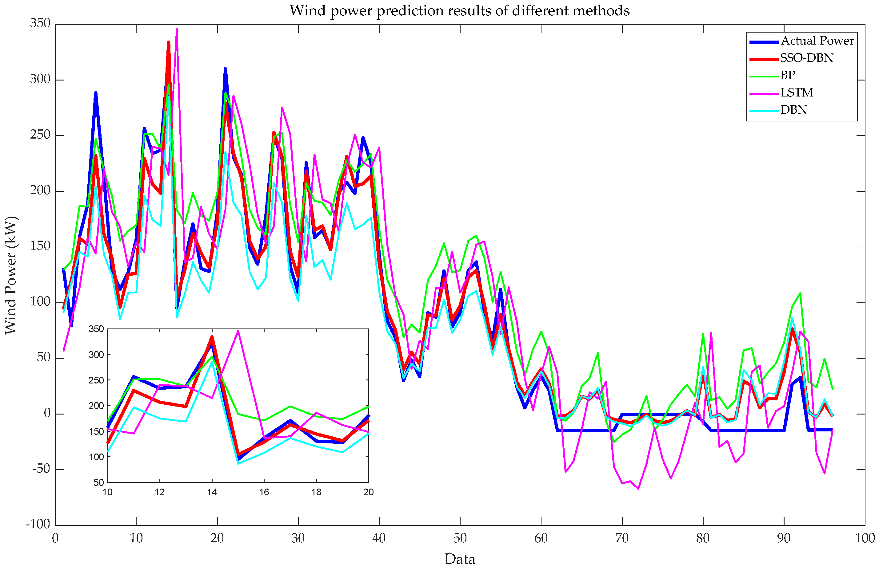
4.1.2. Comparative Study

To evaluate the performance of the proposed model in wind power prediction, we perform a comparative study in this experiment. Here, the embedded dimension M of the historical power is set at 20. The forecasting results of all methods are given in Figure 8. It can be seen that the proposed SSO-DBN model can track the actual power with less error compared with other approaches. In addition, one can see that the prediction accuracy of the SSO-DBN is higher than that of the original DBN method because of the SSO algorithm. Moreover, the convergence curve of the SSO is given in Figure 9; one can see from Figure 9 that the SSO can converge with the optimal solution with twenty-four iterations, and this result demonstrates that the search efficiency is suitable for wind power prediction.
To clearly show the prediction performance, the prediction evaluation results of the different models in terms of MSE, RMSE, MAE and MAPE are given in Table 3. It can be seen from the results in Table 3 that the results of SSO-DBN are all smaller than those of the other models. The values of MAPE for SSO-DBN, BP, LSTM and DBN without optimization are 0.08392, 0.13489, 0.27937 and 0.19779, respectively. The prediction performance of the proposed SSO-DBN method can be improved by 5.1%, 19.5% and 11.39% in terms of MAPE compared to the latter three. So, it can be known that SSO-DBN has relatively good wind power prediction performance.

4.1.3. Validation of Generalization Performance

To verify the generalization performance of the proposed SSO-DBN model, we perform further experiments with four different test data (the number of each test data is 96), which are obtained from the test dataset with different time stages presented in 3.1,where Test data 1 was obtained from 5:15 on 20 June to 5:00 on 21 June 2022, Test data 2 was obtained from 6:15 on 21 June to 6:00 on 22 June 2022, Test Set 3 was obtained from 19:45 on 23 June to 19:30 on 21 June 2022 and Test Set 4 was obtained from 10:15 on 25 June to 10:00 on 26 June 2022. Here, only the prediction curves of the SSO-DBN method are shown for different test data in Figure 10. It can be seen from Figure 10 that the prediction results of the SSO-DBN are still relatively good for different test data, which demonstrates that the proposed SSO-DBN has outstanding tracking and generalization ability. In addition, the evaluation index results of all methods have been listed in Table 4, and one can see that the proposed method has better forecasting accuracy than other approaches for different test data.

4.2. PV Power Forecasting

In this subsection, we conduct further PV power prediction experiments under different conditions to verify the performance of the proposed SSO-DBN method. Without other special instructions, the embedded dimension of the historical power in the following experiments is 16.

4.2.1. Testing the Prediction Performance Considering Different Inputs

As discussed in Section 4.1.1, this subsection will perform experiments to investigate the different factors for the prediction performance of the proposed SSO-DBN. Here, the influencing factors, including GHR, DHR, WTC and WRH, are used to construct different combinations used as the input of the proposed model. The prediction results under different inputs are shown in Figure 11, and one can observe that different inputs generate obvious gaps in prediction results. We see that outstanding prediction results can be obtained when the GHR, DHR, WTC and WRH are all used as the input, because they all have positive correlations with the PV power, as seen in Section 3.2. Furthermore, one can see that poor results are obtained when only the WRH is used as the input because it has a lower correlation coefficient. According to the analysis, the combination of GHR, DHR, WTC and WRH will be used as part of the input in the following experiments.

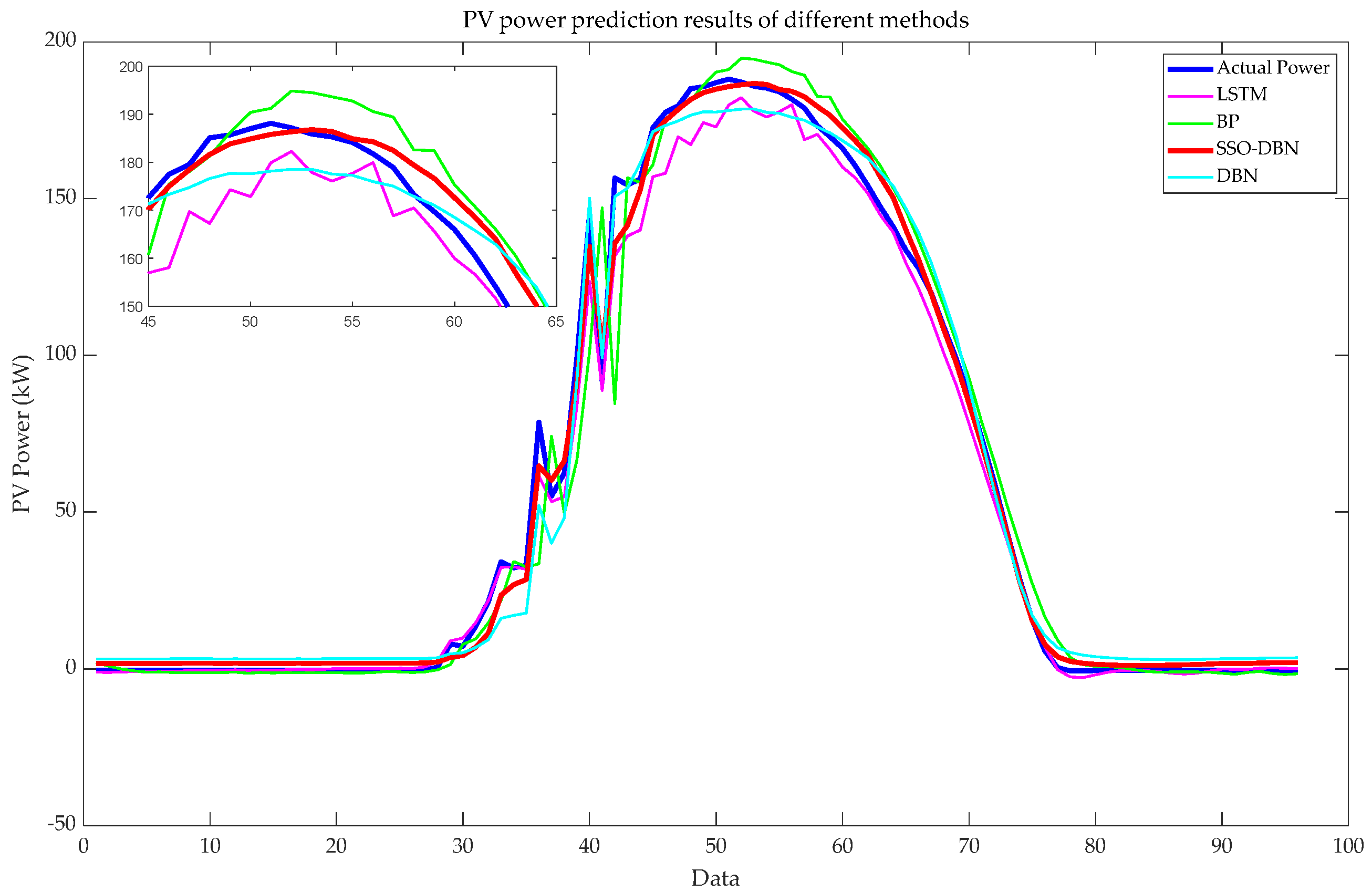
4.2.2. Comparative Study

To further evaluate the performance of the SSO-DBN in PV power prediction, we perform a comparative study with the BP, LSTM and DBM methods. Here, the input is comprised of historical power and four other influencing factors. Figure 12 shows the prediction results of each prediction model. As can be seen from Figure 12, the proposed SSO-DBN can also achieve better forecasting accuracy than other methods, which demonstrates that the proposed prediction model can capture the nonlinear characteristics of the full day’s PV power reasonably well. At the same time, the convergence curve of the SSO in this case is given in Figure 13. We observe that the SSO can converge at the sixty-fifth iteration, which shows good efficiency of the SSO. In addition, since the results of the different evaluation indexes are given in Table 5, one can also know that the proposed SSO-DBN performs better than other methods in this case. The values of MAPE for SSO-DBN, BP, LSTM and DBN without optimization are 0.038172, 0.061008, 0.079889 and 0.046594, respectively. The SSO-DBN can improve the prediction performance by 2.28%, 4.17% and 0.84% compared to the latter three.

4.2.3. Validation of the Generalization Performance

In order to verify the generalization performance of the proposed method, four different test data (the length of each test data is 96) were obtained from the original PV power test dataset, where Test Set 1 was obtained from 0:30 on 8 March to 0:15 on 9 March 2017; Test Set 2 was obtained from 1:30 on 9 March to 1:15 on 10 March 2017; Test Set 3 was obtained from 0:00 on 10 March to 23:45 on 11 March 2017; and Test Set 4 was obtained from 1:00 on 11 March to 0:45 on 12 March 2017. The prediction results under different test sets are given in Figure 14a–d. From the results, we can also find that the proposed SSO-DBN method can obtain a good prediction curve close to the actual power. This result demonstrates that it has good capabilities of tracking and generation. Furthermore, the results of evaluation indexes for all methods under different test datasets are listed in Table 6, and one can also obtain the same conclusion as mentioned above, which shows the superiority of the proposed SSO-DBN method again.

5. Conclusions

Power forecasting is an important technology for the utilization of renewable energy sources, and it is usually faced with the problem of accuracy. In this article, a novel renewable energy prediction model for wind power and PV power was developed by the deep belief network (DBN) with the swarm spider optimization (SSO) method. DBN has a multilayer neural network structure, and it is a multilayer probabilistic machine learning model, which can address the problems of gradient disappearance, the fact of being time-consuming and the large demand for training data. Therefore, it was utilized as the prediction model in this work. In addition, the number of hidden layer nodes as a crucial hyper-parameter of the DBN significantly affects its efficiency, and thus, an outstanding meta-learning method, called SSO, was utilized to select the optimal hyper-parameters of the DBN so as to further improve the prediction accuracy. The meteorological data were selected using Spearman correlation analysis to obtain input features data with a high correlation with power generation. Finally, the input features and the output power were used to construct the training data to train the proposed SSO-DBN model. After training, the model performance was validated using 2022 data from a wind farm in northwest China and 2016 PV data from the Australian Solar Energy Centre. Based on various experiments conducted on the wind power prediction and PV power prediction cases, the experiments demonstrate that the developed SSO-DBN can perform relatively well compared to BP, LSTM and DBN without optimization.
In the future, this will enable us to perform a study where a regularization term will be added with the loss of the DBN to solve the overfitting problem. Furthermore, the proposed model with seq-2-seq form will be introduced into the ensemble learning framework to further enhance its prediction accuracy. In addition, the probabilistic benchmarks test [54] will be used to evaluate the performance of the forecasting method for renewable energy power prediction in our future work.

Author Contributions

Conceptualization, Y.W. and H.Z.; methodology, Y.W., J.D. and R.Z.; software, J.D., L.Q. and Y.D.; validation, Y.W., H.Z. and S.F.; formal analysis, Y.W., J.D. and L.Q.; investigation, Y.W. and H.Z.; data curation, Y.W., J.D. and Y.D.; writing—original draft preparation, Y.W., J.D., L.Q. and Y.D.; writing—review and editing, Y.W., J.D. and S.F. All authors have read and agreed to the published version of the manuscript.

Funding

This research was funded by China Power Engineering Consulting Group Project (grant number GSKJ2D01 2021).

Data Availability Statement

Not applicable.

Acknowledgments

We would like to thank anonymous reviewers for reviewing the manuscript.

Conflicts of Interest

The authors declare no conflict of interest.

References

  1. Choi, S.H.; Manousiouthakis, V.I. Modeling the Carbon Cycle Dynamics and the Greenhouse Effect. Ifac-Papersonline 2022, 55, 424–428. [Google Scholar] [CrossRef]
  2. Zhou, Q.; Ma, Y.; Lv, Q.; Zhang, R.; Wang, W.; Yang, S. Short-Term Interval Prediction of Wind Power Based on KELM and a Universal Tabu Search Algorithm. Sustainability 2022, 14, 10779. [Google Scholar] [CrossRef]
  3. Wu, Z.; Pan, F.; Li, D.; He, H.; Zhang, T.; Yang, S. Prediction of Photovoltaic Power by the Informer Model Based on Convolutional Neural Network. Sustainability 2022, 14, 13022. [Google Scholar] [CrossRef]
  4. Ahmad, F.; Alam, M.S.; Shariff, S.M.; Krishnamurthy, M. A Cost-Efficient Approach to EV Charging Station Integrated Community Microgrid: A Case Study of Indian Power Market. IEEE Trans. Transp. Electrif. 2019, 5, 200–214. [Google Scholar] [CrossRef]
  5. Boudia, S.M.; Yakoubi, A.; Guerri, O. Wind Resource Assessment in The Western Part of Algerian Highlands, Case Study of El-Bayadh. In Proceedings of the 2018 International Conference on Wind Energy and Applications in Algeria (ICWEAA), Algiers, Algeria, 6–7 November 2018. [Google Scholar]
  6. Zhu, X.; Li, S.; Li, Y.; Fan, J. Research progress of the ultra-short term power forecast for PV power generation: A review. In Proceedings of the 2021 33rd Chinese Control and Decision Conference (CCDC), Kunming, China, 22–24 May 2021; pp. 1419–1424. [Google Scholar]
  7. Tu, C.-S.; Tsai, W.-C.; Hong, C.-M.; Lin, W.-M. Short-Term Solar Power Forecasting via General Regression Neural Network with Grey Wolf Optimization. Energies 2022, 15, 6624. [Google Scholar] [CrossRef]
  8. Hanifi, S.; Lotfian, S.; Zare-Behtash, H.; Cammarano, A. Offshore Wind Power Forecasting—A New Hyperparameter Optimisation Algorithm for Deep Learning Models. Energies 2022, 15, 6919. [Google Scholar] [CrossRef]
  9. Sun, G.; Jiang, C.; Cheng, P.; Liu, Y.; Wang, X.; Fu, Y.; He, Y. Short-term wind power forecasts by a synthetical similar time series data mining method. Renew. Energy 2018, 115, 575–584. [Google Scholar] [CrossRef]
  10. Xiyun, Y.; Xue, M.; Guo, F.; Huang, Z.; Jianhua, Z. Wind power probability interval prediction based on bootstrap quantile regression method. In Proceedings of the 2017 Chinese Automation Congress (CAC), Jinan, China, 20–22 October 2017. [Google Scholar]
  11. Wang, C.-N.; Dang, T.-T.; Nguyen, N.-A.; Wang, J.-W. A combined Data Envelopment Analysis (DEA) and Grey Based Multiple Criteria Decision Making (G-MCDM) for solar PV power plants site selection: A case study in Vietnam. Energy Rep. 2022, 8, 1124–1142. [Google Scholar] [CrossRef]
  12. Khasanzoda, N.; Zicmane, I.; Beryozkina, S.; Safaraliev, M.; Sultonov, S.; Kirgizov, A. Regression model for predicting the speed of wind flows for energy needs based on fuzzy logic. Renew. Energy 2022, 191, 723–731. [Google Scholar] [CrossRef]
  13. Wang, F.; Chen, P.; Zhen, Z.; Yin, R.; Cao, C.; Zhang, Y.; Duić, N. Dynamic spatio-temporal correlation and hierarchical directed graph structure based ultra-short-term wind farm cluster power forecasting method. Appl. Energy 2022, 323, 119579. [Google Scholar] [CrossRef]
  14. Li, Z.; Luo, X.; Liu, M.; Cao, X.; Du, S.; Sun, H. Wind power prediction based on EEMD-Tent-SSA-LS-SVM. Energy Rep. 2022, 8, 3234–3243. [Google Scholar] [CrossRef]
  15. Qiang, C.; Qi, X. Research on Trend Analysis and Prediction Algorithm Based on Time Series. In Proceedings of the 2019 3rd International Conference on Electronic Information Technology and Computer Engineering (EITCE), Xiamen, China, 18–20 October 2019. [Google Scholar]
  16. Wu, F.; Cattani, C.; Song, W.; Zio, E. Fractional ARIMA with an improved cuckoo search optimization for the efficient Short-term power load forecasting. Alex. Eng. J. 2020, 59, 3111–3118. [Google Scholar] [CrossRef]
  17. Liu, X.; Lin, Z.; Feng, Z. Short-term offshore wind speed forecast by seasonal ARIMA—A comparison against GRU and LSTM. Energy 2021, 227, 120492. [Google Scholar] [CrossRef]
  18. Huang, Z.; Huang, J.; Min, J. SSA-LSTM: Short-Term Photovoltaic Power Prediction Based on Feature Matching. Energies 2022, 15, 7806. [Google Scholar] [CrossRef]
  19. Xing, Y.; Lien, F.-S.; Melek, W.; Yee, E. A Multi-Hour Ahead Wind Power Forecasting System Based on a WRF-TOPSIS-ANFIS Model. Energies 2022, 15, 5472. [Google Scholar] [CrossRef]
  20. Donti, P.L.; Kolter, J.Z. Machine Learning for Sustainable Energy Systems. Annu. Rev. Environ. Resour. 2021, 46, 719–747. [Google Scholar] [CrossRef]
  21. Yang, X.; Wang, S.; Peng, Y.; Chen, J.; Meng, L. Short-term photovoltaic power prediction with similar-day integrated by BP-AdaBoost based on the Grey-Markov model. Electr. Power Syst. Res. 2023, 215, 108966. [Google Scholar] [CrossRef]
  22. Zhang, Y.; Chen, B.; Pan, G.; Zhao, Y. A novel hybrid model based on VMD-WT and PCA-BP-RBF neural network for short-term wind speed forecasting. Energy Convers. Manag. 2019, 195, 180–197. [Google Scholar] [CrossRef]
  23. Abdoos, A.A. A new intelligent method based on combination of VMD and ELM for short term wind power forecasting. Neurocomputing 2016, 203, 111–120. [Google Scholar] [CrossRef]
  24. Ewees, A.A.; Al-Qaness, M.A.; Abualigah, L.; Elaziz, M.A. HBO-LSTM: Optimized long short term memory with heap-based optimizer for wind power forecasting. Energy Convers. Manag. 2022, 268, 116022. [Google Scholar] [CrossRef]
  25. Li, Z.; Luo, X.; Liu, M.; Cao, X.; Du, S.; Sun, H. Short-term prediction of the power of a new wind turbine based on IAO-LSTM. Energy Rep. 2022, 8, 9025–9037. [Google Scholar] [CrossRef]
  26. Wang, L.; Mao, M.; Xie, J.; Liao, Z.; Zhang, H.; Li, H. Accurate solar PV power prediction interval method based on frequency-domain decomposition and LSTM model. Energy 2023, 262, 125592. [Google Scholar] [CrossRef]
  27. Wang, F.; Xuan, Z.; Zhen, Z.; Li, K.; Wang, T.; Shi, M. A day-ahead PV power forecasting method based on LSTM-RNN model and time correlation modification under partial daily pattern prediction framework. Energy Convers. Manag. 2020, 212, 112766. [Google Scholar] [CrossRef]
  28. Niu, Z.; Yu, Z.; Tang, W.; Wu, Q.; Reformat, M. Wind power forecasting using attention-based gated recurrent unit network. Energy 2020, 196, 117081. [Google Scholar] [CrossRef]
  29. Farah, S.; A, W.D.; Humaira, N.; Aneela, Z.; Steffen, E. Short-term multi-hour ahead country-wide wind power prediction for Germany using gated recurrent unit deep learning. Renew. Sustain. Energy Rev. 2022, 167, 112700. [Google Scholar] [CrossRef]
  30. Liu, H.; Han, H.; Sun, Y.; Shi, G.; Su, M.; Liu, Z.; Wang, H.; Deng, X. Short-term wind power interval prediction method using VMD-RFG and Att-GRU. Energy 2022, 251, 123807. [Google Scholar] [CrossRef]
  31. Dai, Y.; Wang, Y.; Leng, M.; Yang, X.; Zhou, Q. LOWESS smoothing and Random Forest based GRU model: A short-term photovoltaic power generation forecasting method. Energy 2022, 256, 124661. [Google Scholar] [CrossRef]
  32. Li, Q.; Zhang, X.; Ma, T.; Liu, D.; Wang, H.; Hu, W. A Multi-step ahead photovoltaic power forecasting model based on TimeGAN, Soft DTW-based K-medoids clustering, and a CNN-GRU hybrid neural network. Energy Rep. 2022, 8, 10346–10362. [Google Scholar] [CrossRef]
  33. Gao, Y.; Li, Y.; Zhu, Y.; Wu, C.; Gu, D. Power quality disturbance classification under noisy conditions using adaptive wavelet threshold and DBN-ELM hybrid model. Electr. Power Syst. Res. 2021, 204, 107682. [Google Scholar] [CrossRef]
  34. Gao, S.; Xu, L.; Zhang, Y.; Pei, Z. Rolling bearing fault diagnosis based on SSA optimized self-adaptive DBN. ISA Trans. 2021, 128, 485–502. [Google Scholar] [CrossRef]
  35. Mellit, A.; Pavan, A.M.; Lughi, V. Deep learning neural networks for short-term photovoltaic power forecasting. Renew. Energy 2021, 172, 276–288. [Google Scholar] [CrossRef]
  36. Akbal, Y.; Ünlü, K.D. A univariate time series methodology based on sequence-to-sequence learning for short to midterm wind power production. Renew. Energy 2022, 200, 832–844. [Google Scholar] [CrossRef]
  37. Hinton, G.E.; Salakhutdinov, R.R. Reducing the Dimensionality of Data with Neural Networks. Science 2006, 313, 504–507. [Google Scholar] [CrossRef] [PubMed] [Green Version]
  38. Liu, F.; Wang, S.; Zhang, Y. Survey on deep belief network model and its applications. Comput. Eng. Appl. 2018, 54, 11–18. [Google Scholar]
  39. Li, Y.; Peng, T.; Hua, L.; Ji, C.; Ma, H.; Nazir, M.S.; Zhang, C. Research and application of an evolutionary deep learning model based on improved grey wolf optimization algorithm and DBN-ELM for AQI prediction. Sustain. Cities Soc. 2022, 87, 104209. [Google Scholar] [CrossRef]
  40. Li, J.; Wang, W.; Chen, G.; Han, Z. Spatiotemporal assessment of landslide susceptibility in Southern Sichuan, China using SA-DBN, PSO-DBN and SSA-DBN models compared with DBN model. Adv. Space Res. 2022, 69, 3071–3087. [Google Scholar] [CrossRef]
  41. Ma, Y.; Li, Y.; Yue, S.; Sun, H.; Yang, M. Hybrid intelligent hysteresis model based on DBN-DNN algorithm and fusion Preisach operator. J. Magn. Magn. Mater. 2021, 544, 168663. [Google Scholar] [CrossRef]
  42. Wang, K.; Qi, X.; Liu, H.; Song, J. Deep belief network based k-means cluster approach for short-term wind power forecasting. Energy 2018, 165, 840–852. [Google Scholar] [CrossRef]
  43. Yuan, W.; Tang, Z.; Bu, B.; Cao, S. A Novel Hybrid Short-Term Wind Power Prediction Framework Based on Singular Spectrum Analysis and Deep Belief Network Utilized Improved Adaptive Genetic Algorithm. In Proceedings of the 2021 3rd International Conference on Industrial Artificial Intelligence (IAI), Shenyang, China, 8–11 November 2021; pp. 1–6. [Google Scholar] [CrossRef]
  44. Tao, Y.; Chen, H. A hybrid wind power prediction method. In Proceedings of the 2016 IEEE Power and Energy Society General Meeting (PESGM), Boston, MA, USA, 17–21 July 2016. [Google Scholar]
  45. Wang, X.; Yang, Y.; Li, C. Deep Belief Network Based Multi-Dimensional Phase Space for Short-Term Wind Speed Forecasting. In Proceedings of the 2018 International Conference on Sensing, Diagnostics, Prognostics, and Control (SDPC), Xi’an, China, 15–17 August 2018; pp. 204–208. [Google Scholar] [CrossRef]
  46. Wei, H.; Liu, X.; Cao, W.; Ye, G.; Jiang, X.; He, Y. Ultra-short-term Wind Power Forecasting Based on Deep Belief Network and Wavelet Denoising. In Proceedings of the 2021 IEEE 4th International Electrical and Energy Conference (CIEEC), Wuhan, China, 28–30 May 2021; pp. 1–6. [Google Scholar] [CrossRef]
  47. Hu, S.; Xiang, Y.; Huo, D.; Jawad, S.; Liu, J. An improved deep belief network based hybrid forecasting method for wind power. Energy 2021, 224, 120185. [Google Scholar] [CrossRef]
  48. Duan, J.; Wang, P.; Ma, W.; Fang, S.; Hou, Z. A novel hybrid model based on nonlinear weighted combination for short-term wind power forecasting. Int. J. Electr. Power Energy Syst. 2021, 134, 107452. [Google Scholar] [CrossRef]
  49. Wang, H.-Y.; Chen, B.; Pan, D.; Lv, Z.-A.; Huang, S.-Q.; Khayatnezhad, M.; Jimenez, G. Optimal wind energy generation considering climatic variables by Deep Belief network (DBN) model based on modified coot optimization algorithm (MCOA). Sustain. Energy Technol. Assess. 2022, 53, 102744. [Google Scholar] [CrossRef]
  50. Cuevas, E.; Cienfuegos, M.; Zaldívar, D.; Pérez-Cisneros, M. A swarm optimization algorithm inspired in the behavior of the social-spider. Expert Syst. Appl. 2013, 40, 6374–6384. [Google Scholar] [CrossRef] [Green Version]
  51. Dey, A.; Dey, S.; Bhattacharyya, S.; Platos, J.; Snasel, V. Novel quantum inspired approaches for automatic clustering of gray level images using Particle Swarm Optimization, Spider Monkey Optimization and Ageist Spider Monkey Optimization algorithms. Appl. Soft Comput. 2019, 88, 106040. [Google Scholar] [CrossRef]
  52. Ben, U.C.; Akpan, A.E.; Urang, J.G.; Akaerue, E.I.; Obianwu, V.I. Novel methodology for the geophysical interpretation of magnetic anomalies due to simple geometrical bodies using social spider optimization (SSO) algorithm. Heliyon 2022, 8, e09027. [Google Scholar] [CrossRef] [PubMed]
  53. Yuan, X.; Gu, Y.; Wang, Y. Supervised Deep Belief Network for Quality Prediction in Industrial Processes. IEEE Trans. Instrum. Meas. 2020, 70, 1–11. [Google Scholar] [CrossRef]
  54. Martinez, R.G. How good is good? probabilistic benchmarks and nanofinance+. arXiv 2021, arXiv:2103.01669. [Google Scholar]
Figure 1. (a) Structural diagram of the RBM; (b) Structure diagram of DBN.
Processes 11 01001 g001
Figure 2. Flowchart of SSO algorithm.
Processes 11 01001 g002
Figure 3. Wind power and impact factor data curves in one day.
Processes 11 01001 g003
Figure 4. PV power and impact factor data curves in one day.
Processes 11 01001 g004
Figure 5. Flow chart of the SSO-DBN forecasting model.
Processes 11 01001 g005
Figure 6. Overall flowchart of the renewable energy power prediction.
Processes 11 01001 g006
Figure 7. Wind power prediction results under different inputs.
Processes 11 01001 g007
Figure 8. Wind power prediction results of different methods.
Processes 11 01001 g008
Figure 9. Convergence curve of SSO (Wind Power).
Processes 11 01001 g009
Figure 10. Predicted results of the proposed model for different test sets. Where, (a) is the result of set 1, (b) is the result of set 2, (c) is the result of set 3, and (d) is the result of set 4.
Processes 11 01001 g010
Figure 11. PV power prediction results under different inputs.
Processes 11 01001 g011
Figure 12. PV power prediction results of different methods.
Processes 11 01001 g012
Figure 13. Convergence curve of SSO (PV Power).
Processes 11 01001 g013
Figure 14. Prediction results of PV power under different test sets (ad).
Processes 11 01001 g014
Table 1. SCC results between the wind power and other influencing factors.
Influencing FactorsAverage Paddle
Angle
Average Pitch Speed of Paddle (1)Average Pitch Speed of Paddle (2)Maximum Wind Speed
Correlation coefficient−0.19910.00320.00400.8821
Influencing FactorsMinimum Wind SpeedAverage Wind SpeedAverage Wind DirectionAverage Outdoor Temperature
Correlation Coefficient0.85920.9093−0.0786−0.2952
Table 2. SCC results between the PV power and other influencing factors.
Influencing FactorsGlobal Horizontal RadiationDiffuse Horizontal
Radiation
Weather Temperature CelsiusWeather Relative Humidity
Correlation Coefficient0.81960.76800.7418−0.6108
Table 3. Prediction results evaluation form (Wind Power).
ModelMSERMSEMAEMAPE
BP1425.637.757832.08980.13489
LSTM3199.556.564642.82760.27937
DBN1031.432.115625.13420.19779
SSO-DBN423.1320.570215.23060.08392
Table 4. Prediction results of evaluation index (wind).
Test Set 1ModelMSERMSEMAEMAPE
DBN124,116352.3017284.3730.13633
BP48,960221.2694174.67410.085356
LSTM307,442554.4751422.63090.21699
SSO-DBN43,912209.5526166.19280.079677
Test Set 2ModelMSERMSEMAEMAPE
DBN46,720216.149168.90780.087231
BP135,712368.3912280.440.15921
LSTM348,741590.5431457.14090.25074
SSO-DBN24,042155.0563115.38860.061968
Test Set 3ModelMSERMSEMAEMAPE
DBN10,807103.961181.44490.20845
BP11,598107.697687.29350.18541
LSTM34,440185.5827131.6170.33576
SSO-DBN577275.977351.98160.13823
Test Set 4ModelMSERMSEMAEMAPE
DBN26,797163.6992137.04560.35413
BP943597.13862.9950.17088
LSTM24,355156.0626112.91450.25035
SSO-DBN521072.182249.31070.13241
Table 5. Prediction results evaluation form (PV Power).
ModelMSERMSEMAEMAPE
BP47.64556.90263.99770.061008
LSTM173.719313.18036.49630.079889
DBN48.65326.97525.60780.046594
SSO-DBN29.23725.40713.20730.038172
Table 6. Evaluation index results under different test sets.
Test Set 1ModelMSERMSEMAEMAPE
BP4.57692.13941.8740.06363
LSTM67.4068.21016.00990.29398
DBN9.283.04632.26910.10342
SSO-DBN3.08031.75511.35890.052383
Test Set 2ModelMSERMSEMAEMAPE
BP24.98294.99834.61870.051809
LSTM117.994510.86255.14220.31958
DBN9.00963.00162.3640.084287
SSO-DBN5.04572.24631.84530.060033
Test Set 3ModelMSERMSEMAEMAPE
BP4.99112.23411.65940.04845
LSTM239.190215.46586.08810.35011
DBN13.51673.67652.84210.098
SSO-DBN8.08522.84341.97870.072879
Test Set 4ModelMSERMSEMAEMAPE
BP81.44159.02455.2730.10024
LSTM961.550631.008915.84320.29904
DBN58.23687.63134.750.085909
SSO-DBN43.89416.62533.9640.075145
Disclaimer/Publisher’s Note: The statements, opinions and data contained in all publications are solely those of the individual author(s) and contributor(s) and not of MDPI and/or the editor(s). MDPI and/or the editor(s) disclaim responsibility for any injury to people or property resulting from any ideas, methods, instructions or products referred to in the content.

