Article

A Combined Gated Recurrent Unit and Multi-Layer Perception Neural Network Model for Predicting Shale Gas Production

1
State Key Laboratory of Shale Oil and Gas Enrichment Mechanisms and Effective Development, Beijing 100083, China
2
Sinopec Key Laboratory of Shale Oil/Gas Exploration and Production Technology, Beijing 100083, China
3
State Key Laboratory of Petroleum Resources and Prospecting, China University of Petroleum (Beijing), Beijing 102249, China
*
Author to whom correspondence should be addressed.
Processes 2023, 11(3), 806; https://doi.org/10.3390/pr11030806
Submission received: 30 January 2023 / Revised: 2 March 2023 / Accepted: 6 March 2023 / Published: 8 March 2023

Abstract

:
Shale gas plays an important role in supplementing energy demand and reducing carbon footprint. A precise and effective prediction of shale gas production is important for optimizing completion parameters. This paper established a gated recurrent unit and multilayer perceptron combined neural network (GRU-MLP model) to forecast multistage fractured horizontal shale gas well production. A nondominated sorting genetic algorithm II (NSGA II) was introduced into the model to enable its automatic architectural optimization. In addition, embedded discrete fracture models (EDFM) and a reservoir simulator were used to generate training datasets. Meanwhile, a sensitivity analysis was carried out to find the variable’s importance and support the history matching. The results illustrated that the GRU-MLP model can precisely and efficiently predict the productivity of multistage fractured horizontal shale gas in a rapid and effective manner. Additionally, the model fits better at peak values of shale gas production. The GRU-MLP hybrid model has a higher accuracy within an acceptable computational time range compared to recurrent neural networks (RNN), long short-term memory (LSTM), and GRU models. The mean absolute percentage error (MAPE) and root mean square percentage error (RMSPE) for shale gas production generated by GRU-MLP model were 3.90% and 3.93%, respectively, values 84.87% and 84.88% smaller than those of the GRU model. Consequently, compared with a purely data-driven method, the physics-constrained data-driven method behaved better. The main results of the study will hopefully contribute to the intelligent development of shale gas production prediction.

1. Introduction

Natural gas is considered to be the cleanest fossil fuel, and the role of shale gas is increasing in terms of the third energy conversion from fossil energy to new energy [1,2]. According to IEA’s World Energy Outlook 2022, the world’s unconventional natural gas production reached 1.185 × 10¹² m3, of which shale gas production accounted for 66.67% in 2021. It is predicted that the natural gas demand in the Stated Policies Scenario will increase to 4.357 × 10¹² m3 by 2050 (Figure 1) [3]. Natural gas produced lower carbon emissions during combustion than oil and coal, and it will play an important role in the future energy mix [4,5]. The electricity sector which is currently the main carbon-emitting sector globally, still uses fossil fuels, such as coal, oil, and natural gas, as the dominant materials to generate electricity [3]. Therefore, shale gas, as a major component of natural gas, contributes to reducing carbon footprint and has huge development potential in energy supply. However, owing to the ultralow porosity and permeability, stimulation methods are necessary to achieve industrial development of shale gas resources [6]. A number of shale gas stimulation methods have been proposed to increase shale gas production, such as supercritical CO2 fracturing [7], application of micro-nanoparticles [8], nitrogen/carbon dioxide injection, and thermal stimulation methods [9]. Hydraulic fracturing, which has been performed efficiently in recent decades, is the main method for shale gas development [10]. Accurate prediction of shale gas production after hydraulic fracturing plays a vital role in evaluating production status and selecting optimal completion methods and parameters. However, the complex multi-scale system containing micro-nano pores and natural and hydraulic fracture networks make the fluid flow in the stimulation area more complicated [11,12]. Therefore, the accurate prediction of shale gas production faces large challenges due to the complex flow mechanism of a complex multi-scale system.
The analytical approach and numerical analysis are traditional approaches to shale gas production prediction [11,13]. The analytical approach establishes a production model based on complex mechanisms, relying on certain assumptions that limit the range of usage. The commonly used approach is decline curve analysis, which is suitable for long-term production prediction, but not for daily production prediction [13]. Numerical analysis considers compositional study and high-dimensional physics, which make models with high accuracy in predicting shale gas production. However, the numerical model faces the challenges of gridding and computational costs, especially dealing with complex fracture networks, history matching, parameter optimization [11], etc.
The first applications of artificial intelligence (AI) in the oil and gas industry trace back to the 1970s [14]. With the rapid development of AI, machine learning (ML) algorithms have been widely applied in petroleum engineering, including reservoir engineering, drilling, completion, production, etc. [15,16,17], and have broad application prospects. Production prediction is an important application of ML algorithms in oil and gas development. Extensive research has been conducted to forecast shale gas production with ML-based algorithms, such as artificial neural networks (ANN), LSTM, the support vector machine (SVM), etc. [2,15,18,19]. Accurate results are obtained frequently and efficiently. Syed et al. compare different ML algorithms, including decision tree (DT), random forest (RF), SVM, and gradient boosting for regression tree (GBRT), and describe their advantages and disadvantages [20]. Nguyen-Le and Shin propose three ANN architectures developed based on 370 stimulation data, including geological and engineering parameters for predicting peak production [21]. ANN contains deep feed-forward neural networks (DFNN). Liu et al. applied DFNN to predict the EUR of shale gas wells in the Weiyuan block. Niu et al. concluded that SVM is the most reliable algorithm for predicting shale gas estimate ultimate recovery (EUR) compared with K-nearest neighbor (KNN), RF, and gradient boosting decision tree [22]. Deep-learning (DL) algorithms represent a branch of ML where RNN is extensively used for time series predictions [23]. LSTM is a variation of RNN which can combine short-term and long-term memory by gating, compared to RNN, which can only remember short-term memory [24]. Zhu et al. applied LSTM to guide shale gas well production. The changing trend of production for the next 10 days can be captured by the LSTM model [13]. Yang et al. used the LSTM model for long-term shale gas production prediction, and it provided the best-fitting effect and smallest error compared to traditional analytical methods [2]. However, data-driven methods rely much more on data collected from the field, and well-accepted physical laws exist [25]. To solve the above disadvantages, some researchers have proposed hybrid physical data approaches, which can be divided into three types according to the physical mechanism and data, one of which is to enforce known physical constraints into the data-driven models [25].
Methods for enforcing physical constraints into data-driven models, have attracted the attention of researchers due to the preservation of field data with high computational efficiency and a low requirement for historical data [15]. Li et al. presented a physics-constrained deep learning method with a combined neural network based on a bidirectional gated recurrent unit (BiGRU) and a deep hybrid neural network (DHNN) for production prediction [26]. Salehi et al. developed a model based on physics-based and data-driven algorithms without considering time series analysis [27]. Park et al. developed a hybrid model by using reservoir simulations to generate training datasets and data-driven ML algorithms [28]. However, the optimization of the automatic model structure requires further research for production prediction. Yang et al. proposed a new physics-constrained data-driven workflow with a GRU-MLP model considering time series analysis and a multiobjective algorithm (NSGA II) which can achieve automatic optimization of the model’s structure [15]. The hybrid model can forecast the coalbed methane (CBM) production accurately, quickly, and stably. However, there are some shortcomings, such as the unevaluated contribution of each feature to the model’s performance.
In summary, numerous studies have been carried out on data-driven shale gas pro-duction prediction; however, the quality and quantity of field data affect its accuracy. The physics-constrained and data-driven model is less commonly used, and physical-constrained data-driven workflows are not well established in production forecasting of shale gas. This study introduces the GRU-MLP model to shale gas production forecasting and evaluates the contributions of each feature to accelerating the history matching process.
In this paper, we first introduce the data preprocessing method, the EDFM, and the neural network. Then, sensitivity analysis is performed to find the variable importance for quick and efficient history matching. Finally, comparisons between different ML algorithms are performed to confirm the accuracy and computational efficiency of the model. This study aims to increase the accuracy of shale gas production prediction, and is anticipated to provide theoretical guidance for intelligent shale gas production.

2. Methodology

2.1. Embedded Discrete Fracture Model

EDFM was developed by Li and Lee to overcome the limits of bi-continuum and discrete fracture models [29]. As the method has been continuously developed and refined by many scholars, the model has been applied in many reservoir simulators [30]. EDFM [31,32,33], as a numerical simulation tool for complex fracture networks, can effectively solve the problems of modeling complex fracture geometries. This method embeds complex hydraulic and natural fractures into matrix blocks by generating extra grids in the computational domain. Based on the fracture well index and non-neighboring connections (NNCs) transmissibility factor, EDFM can model fractures explicitly. Generally, there are three types of NNCs: (1) connection between a matrix block and a fracture segment that penetrates it, (2) connection between fracture segments of the same fracture, and (3) connection between intersecting fracture segments [34].
The advantage of EDFM is that the precision afforded by the discrete fracture model and the efficiency provided by structured gridding is preserved. This study combines EDFM and CMG commercial reservoir simulators to simulate shale gas production with complex fracture geometries.

2.2. GRU-MLP Combined Neural Network

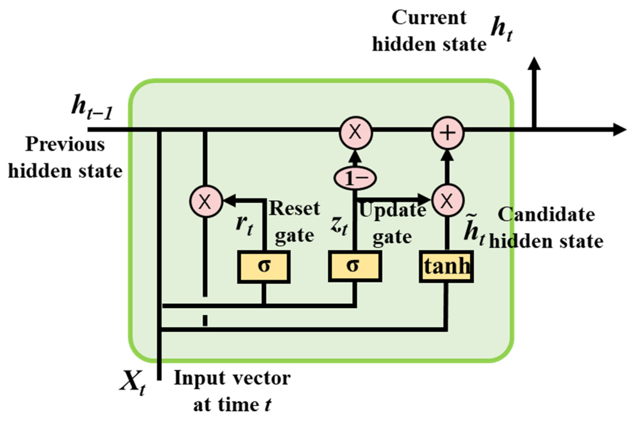
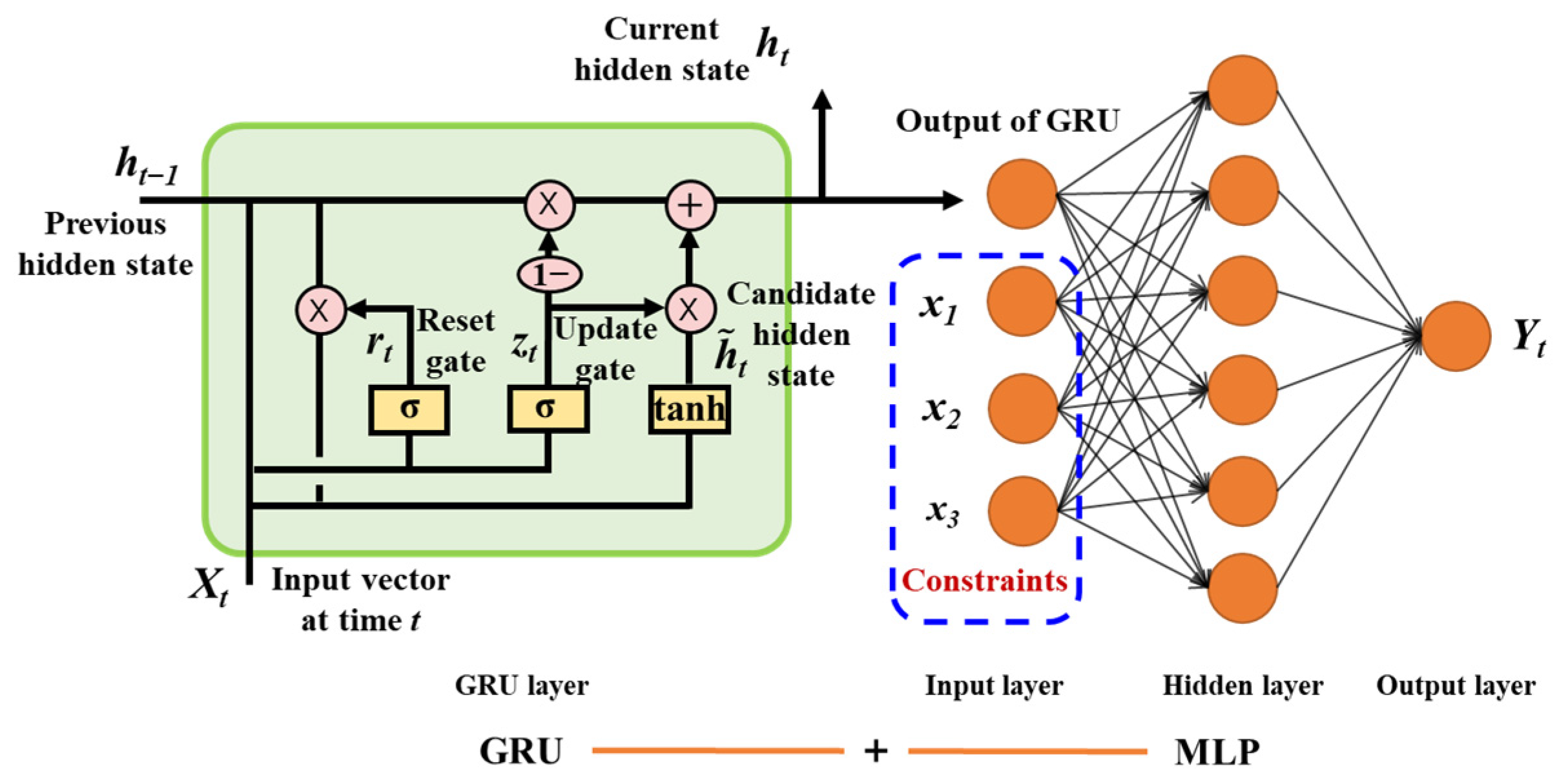
2.2.1. Gated Recurrent Unit (GRU)

RNN is effective and precise in the application of time series predictions [35]. GRU is a variant of LSTM, which is developed based on RNN. GRU is faster when processing information, but a comparable prediction performance is obtained due to the fact that its inner structure is much simpler than that of LSTM [36]. Figure 2 shows the structure of the GRU model. The GRU model includes a reset gate rt and an update gate zt. First, the output ht−1 at the last time step and the new data xt, are introduced into the network as the input. Then, the output is reset by a reset gate to remove the information of ht−1 that is temporarily stored in h ¯ t after adding on xt. The reset gate determines the proportion of ht−1 and h ¯ t when updating ht.

2.2.2. Multilayer Perceptron (MLP)

MLP is a kind of feedforward ANN which consists of an input layer, one or more hidden layers, and an output layer [38]. The complex nonlinear mapping between a group of input and output variables is described by activation functions. The nodes in the next and previous layers are fully connected by weights and nonlinear transfer/activation functions. The input of a node in the next layer is obtained by scaling the output of nodes in the previous layer and feeding forward. The superposition of nonlinear transfer functions enables the MLP to be superior in learning and expressing nonlinear relations [39]. Therefore, the main advantage of MLP is solving complex problems quickly. MLP is a generalization of the perceptron that overcomes the weakness of its inability to recognize linear, inseparable data. MLP also has a better capability to express and learn nonlinear relations. However, MLP does not handle sequence problems well due to the lack of memory function [40].

2.2.3. GRU-MLP Combined Neural Network

Production prediction of multi-fracture horizontal shale gas wells is a complex nonlinear time series prediction problem. Combining the ability of GRU to store long-term sequential data with the flexibility of MLP in handling the nonlinear relationship between input and output data, we applied a new type of combined neural network, the GRU-MLP combined neural network (Figure 3), to predict shale gas production [14]. GRU was employed for the time series task. The main function of GRU is to learn relationships between historical data, expressed as X1, X2, X3, …, X4, and predict the future trend, represented as XT+1. The new inputs of MLP were combined with physical constraints (x1, x2, x3, …, xn) and output generated through the GRU layer, a vector merge layer, and a linear activation layer. The nonlinear relationship between production data and physical constraints was learned by MLP to increase the accuracy of prediction by improving the effects of physical constraints on the production performance. Finally, the production prediction results at time step T + 1 were obtained [41].

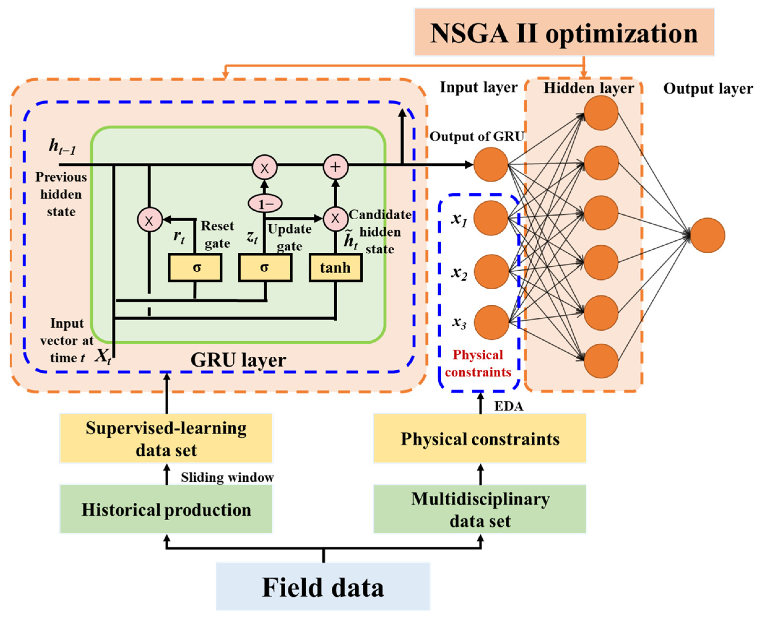
2.2.4. Workflow Based on the GRU-MLP Model

The workflow based on the GRU-MLP is proposed to predict shale gas and water production. Figure 4 illustrates the workflow. First, the field data was collected and preprocessed by exploratory data analysis (EDA) to build a multidisciplinary data set. Second, a supervised-learning data set, obtained from production history data together with a multidisciplinary data set as physical constraints, formed the input of MLP. Third, the GRU-MLP network architecture was optimized by NSGA II and the production performance was forecasted.

3. Field Application

In this section, a shale gas reservoir model and a GRU-MLP model were established. The data were collected from a multistage fractured horizontal shale gas well located at Fuling area in the Sichuan Basin, China. Longmaxi Formation was developed. In November 2012, JY1HF, located at the study area, was drilled with 2.03 × 10⁵ m3 of gas flow rate in the testing process, representing a breakthrough in this area. The cumulative gas production of the area reached 3.4 × 10¹⁰ m3 in 2020 [42]. The well spacing was approximately 600 m and infilled well spacing was reduced to approximately 300 m. First, a reservoir numerical model was established based on field data. Then, sensitivity analysis was performed to find the variable importance to aid history matching. Based on the data generated by history matching, the GRU-MLP model was developed and the model architecture was optimized, with the goals of minimum training time and as few prediction errors as possible.

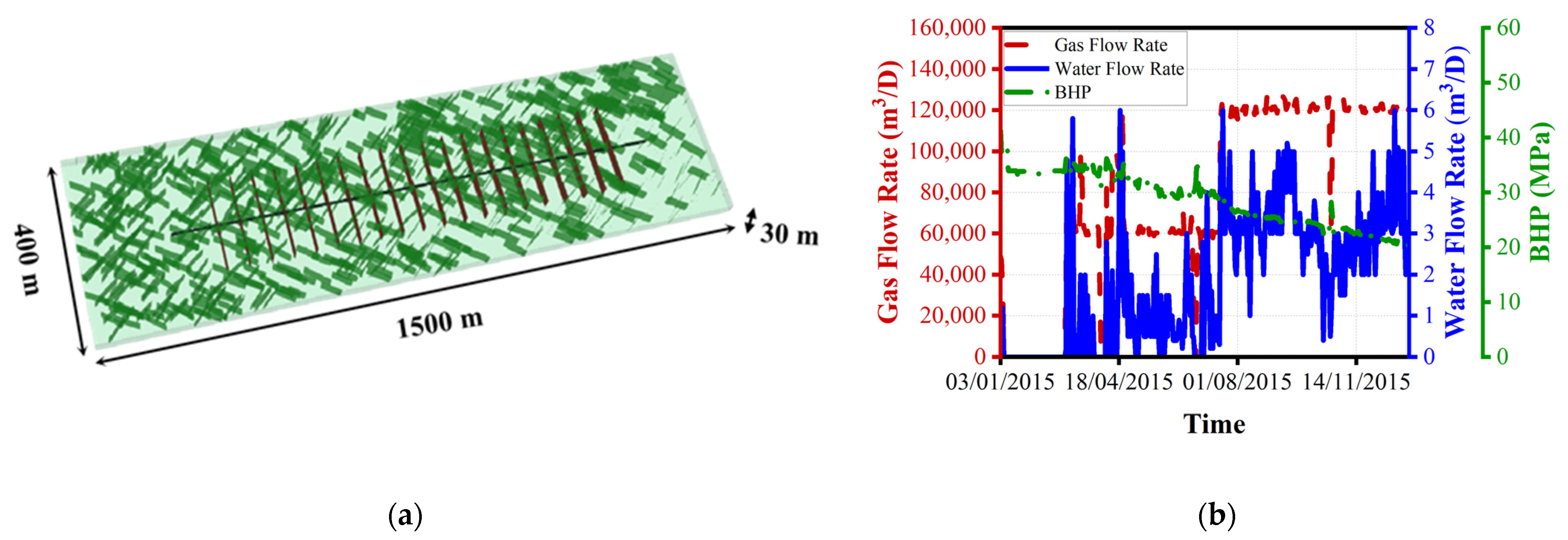
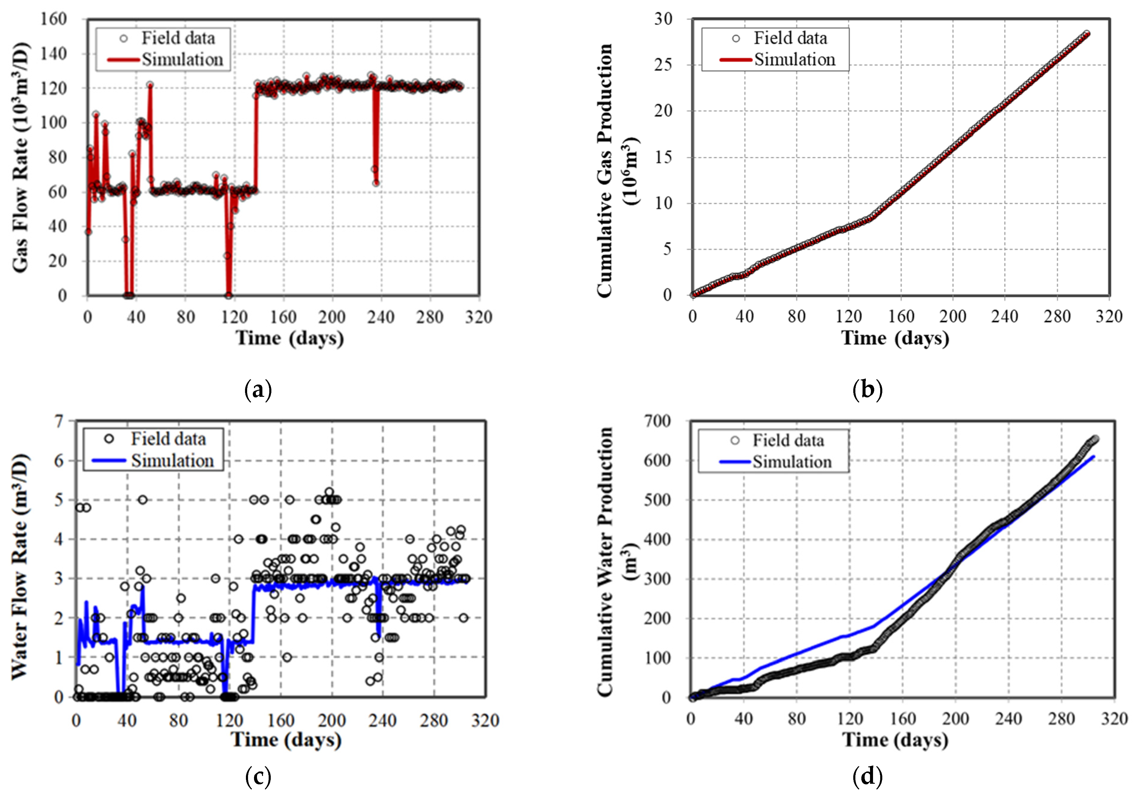
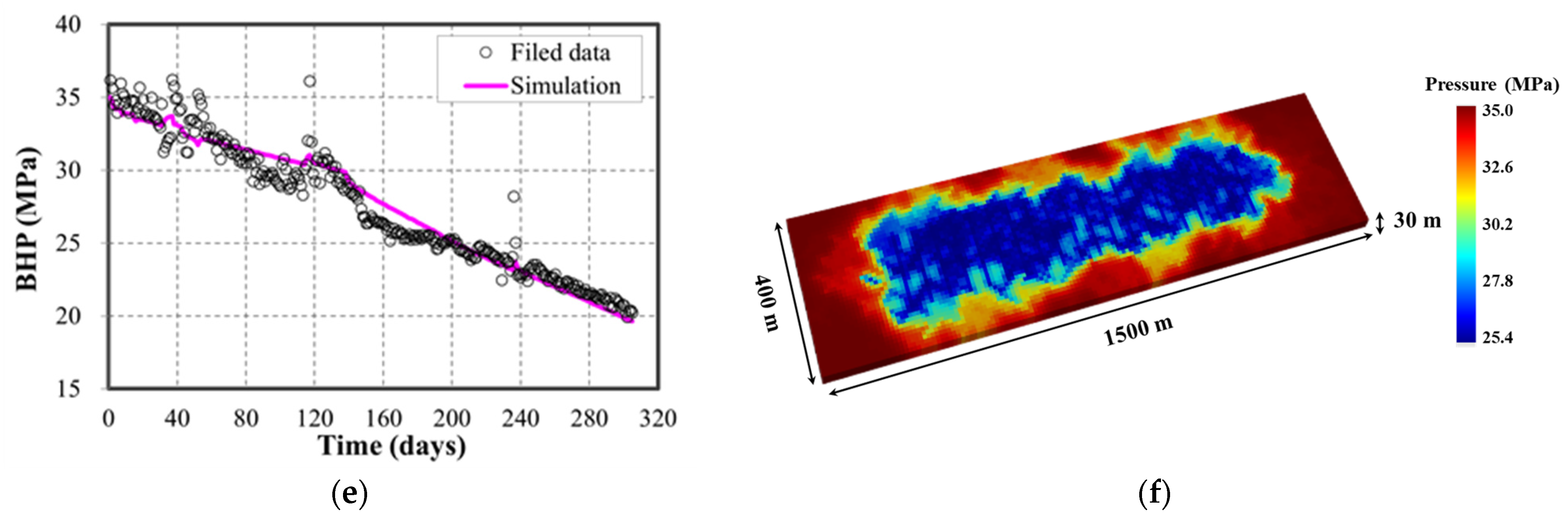
3.1. Reservoir Simulation Model

EDFM has been proven to be feasible in previous studies [34,43]. The model is assumed to involve isothermal seepage with two-phase gas/water flow patterns. In this model, the permeability of the reservoir and the permeability of the fractures are assumed to be functions of pressure. Based on a Cartesian grid system, we established the reservoir model to have dimensions of 1500 m × 400 m × 30 m, representing reservoir length, width, and thickness, respectively. The reservoir model consisted of a horizontal well with 20 hydraulic fractures and spacing between 2 adjacent hydraulic fractures, as shown in Figure 5. The total lateral length of the multistage fractured horizontal shale gas well was 1150 m.
The sensitivity of the base case was investigated to quantify the effect of geologic properties and completion of operational parameters on complex gas–water two-phase flow and shale gas production. The effects of hydraulic fracture parameters, including the half-length and initial conductivity of hydraulic fractures; and the natural fracture properties, including the number and initial conductivity of natural fractures, are presented. Table 1 shows the simulation parameters of sensitivity cases.

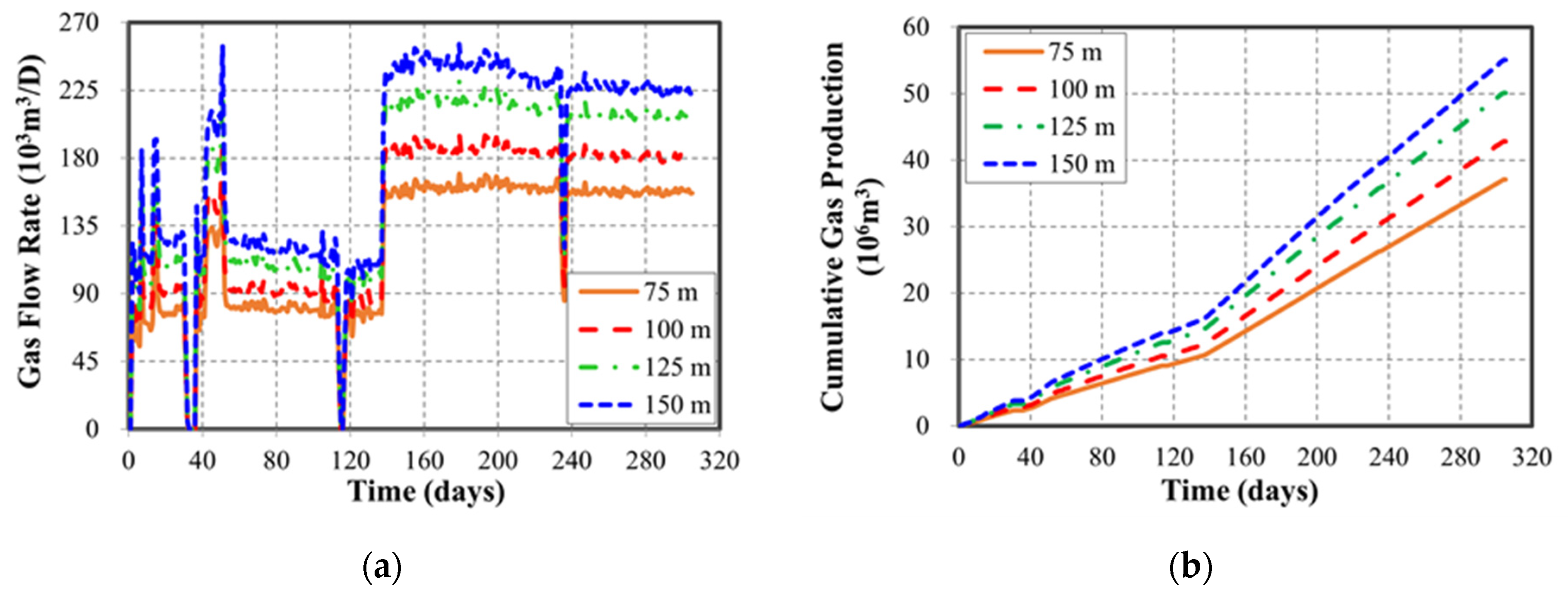
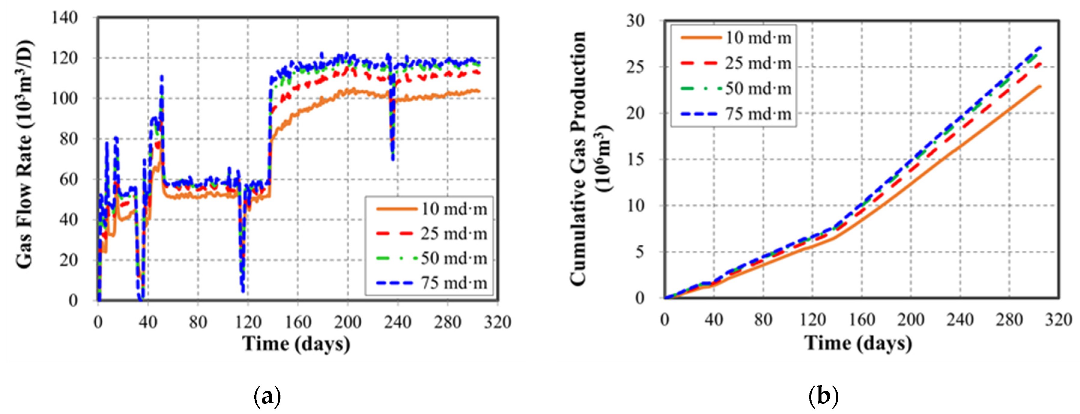
3.1.1. Effect of Hydraulic Fracture

Figure 6 demonstrates that the effects of hydraulic fracture half-length and daily gas production rate grow as the hydraulic fracture half-length increases. As illustrated in Figure 6a, the effect on gas flow rate gradually decreased after 305 days of development due to the hydraulic fracture half-length. The gas production rose sharply around the 140th day. In the absence of other production stimulation measures, the greater the production pressure difference, i.e., the difference between reservoir pressure and bottom hole pressure, the greater the gas flow rate. Figure 6b reveals the effect of hydraulic fracture half-length on cumulative gas production. An increase in hydraulic fracture half-length will further improve the stimulated reservoir volume (SRV), connecting more natural fractures. The cumulative production with a 125 m hydraulic fracture half-length is 5.01 × 10⁷ m3, which is 17.05% higher than a 100 m hydraulic fracture half-length. However, with a hydraulic fracture half-length of 150 m, the cumulative production is 9.82% greater than with one of 125 m. The results reflect that as the hydraulic fracture half-length increases, the growth rate of cumulative gas production slows down. Therefore, the hydraulic fracture half-length needs to be optimized to achieve economic benefits.
The initial conductivity of hydraulic fractures has an impact on the gas flow rate and cumulative gas production of the shale gas well. With the increase in hydraulic fracture conductivity, the gas flow rate rises while the increase rate decreases, as shown in Figure 7a. As production time increases, the fracture conductivity decreases compared to the initial fracture conductivity, and there is a small reduction in daily gas production. However, as the production pressure difference increases, daily gas production rises and the reduction is not significant. The effect of initial hydraulic fracture conductivity on cumulative gas production is shown in Figure 7b. At 305 days, the cumulative production with an initial hydraulic fracture conductivity of 25 mD·m increased by 12.94% over that with an initial hydraulic fracture conductivity of 10 mD·m, while cumulative production increased by only 1.88% when the initial hydraulic fracture conductivity increased from 50 mD·m to 75 mD·m. This represents a significant slowdown in the rate of increase. The transportability of hydraulic fractures improves with increasing hydraulic fracture conductivity. However, the supply ability of shale matrix does not change with increased initial hydraulic fracture conductivity [44]. Therefore, the gas flow rate is slightly affected by the increasing hydraulic fracturing conductivity, especially when the initial hydraulic fracture conductivity is sufficiently large.

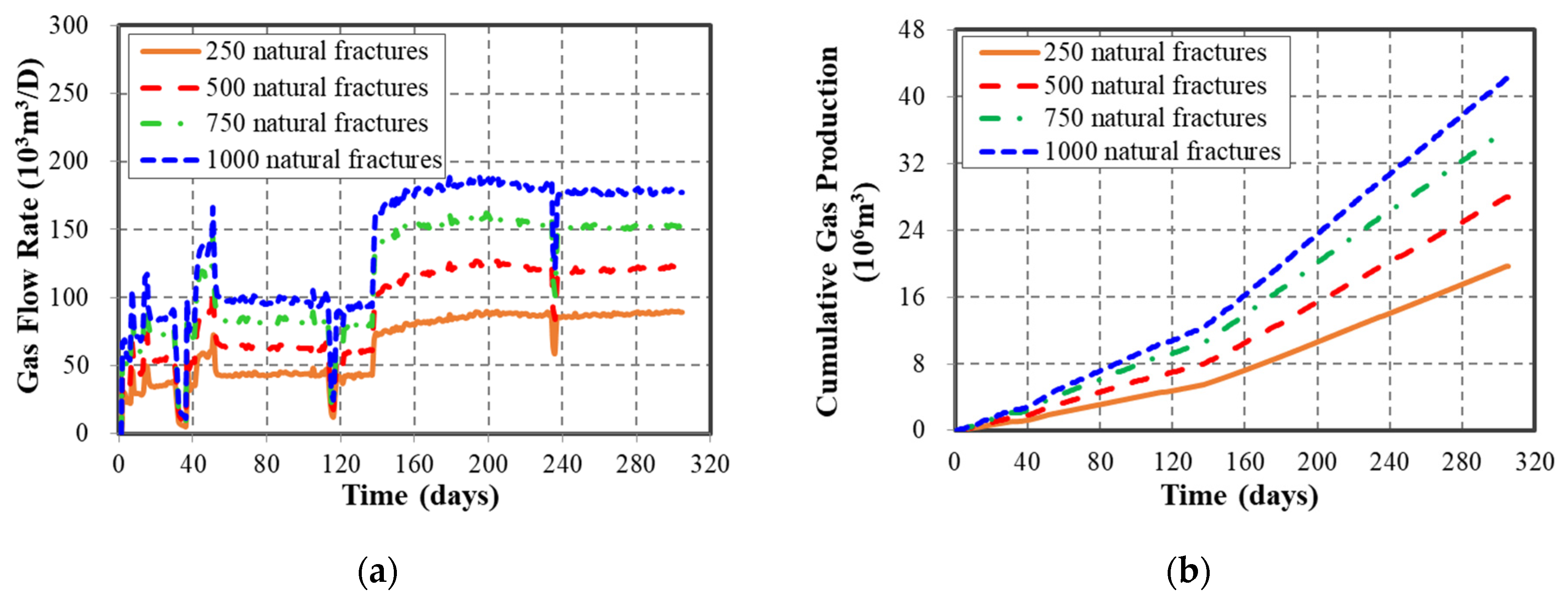
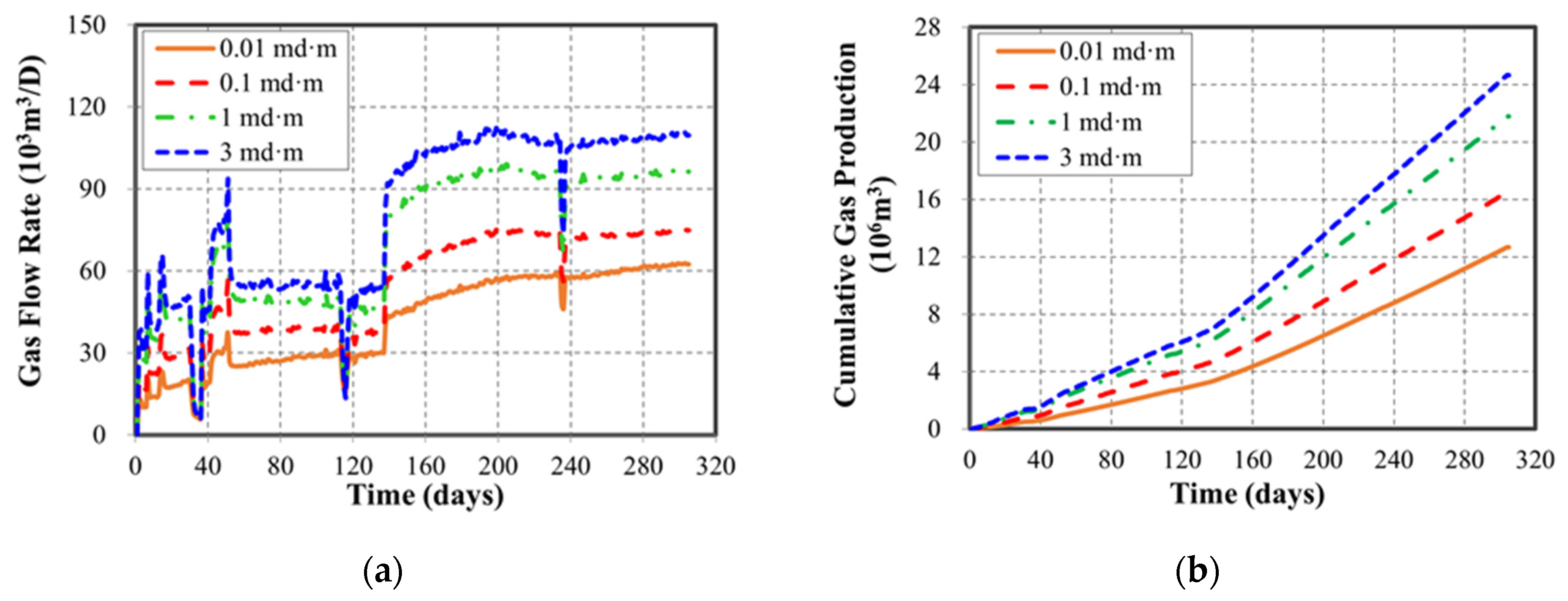
3.1.2. Effect of Natural Fracture

This section discusses the influence of natural fracture parameters in shale gas production. The presence of natural fractures responds positively to gas productivity in certain scenarios. As seen in Figure 8, gas flow rate and cumulative gas production increase with the natural fracture numbers. The reason can be attributed to the fact that more natural fractures increase the contact between rocks, thereby increasing the available drainage area. The gas flow rate surged around the 140th day due to fluctuations in bottom hole pressure. The larger the number of natural fractures, the greater the fluctuation of the gas flow rate. In theory, more natural fractures are beneficial to production; however, this is based on characteristics of open natural fractures.
Gas production is also affected by the initial conductivity of natural fractures, as illustrated in Figure 9. The gas flow rate and cumulative gas production increase with natural fracture conductivity. As the initial natural fracture conductivity increases, more fluid flows from the reservoir into the wellbore through the natural fractures, which communicate with the hydraulic fractures. As production time increases, the initial conductivity of the natural fractures has a noticeable impact on production, and the cumulative gas production increases significantly.

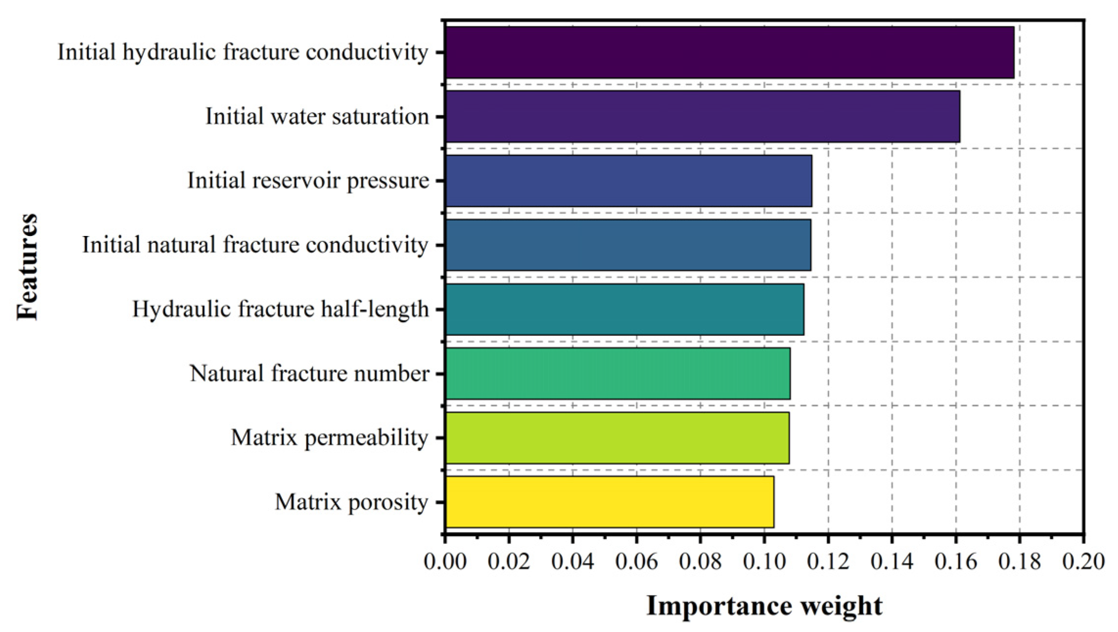
3.1.3. Sensitivity Analysis Results

Due to the inability of the GRU-MLP model to automatically evaluate the importance of different features, the feature importance evaluation of the RNN approach is applied to recognize the importance of each parameter. Once heavy hitters are identified, the less influential parameters can be screened out to decrease the number of history-matching numerical simulations. The unknown parameters have predefined ranges, including, but not limited to, the four fracture parameters described previously. Then, the reservoir is modeled and simulated with the unknown parameters. The results of the simulations are used as inputs for the RNN model, and the importance of the different features is evaluated through the model’s inherent feature importance evaluation. Figure 10 shows the influence of each parameter.

3.1.4. Data Generating

Table 2 presents the result of history matching and input parameters considered in the model. The reservoir has a matrix porosity of 6%, a matrix permeability of 0.0009 mD, and an initial water saturation of 35%. The hydraulic fracture has an initial conductivity of 10 mD·m and a half-length of 100 m. A comparison of the field data with the simulation data is presented in Figure 11. Simulation results of the water flow rate and bottom hole pressure (BHP) illustrate that the results of this model are consistent with the field data. It also verifies the feasibility and accuracy of the model and shows that EDFM has an advantage in producing nonplanar fractures.

3.2. GRU-MLP Model

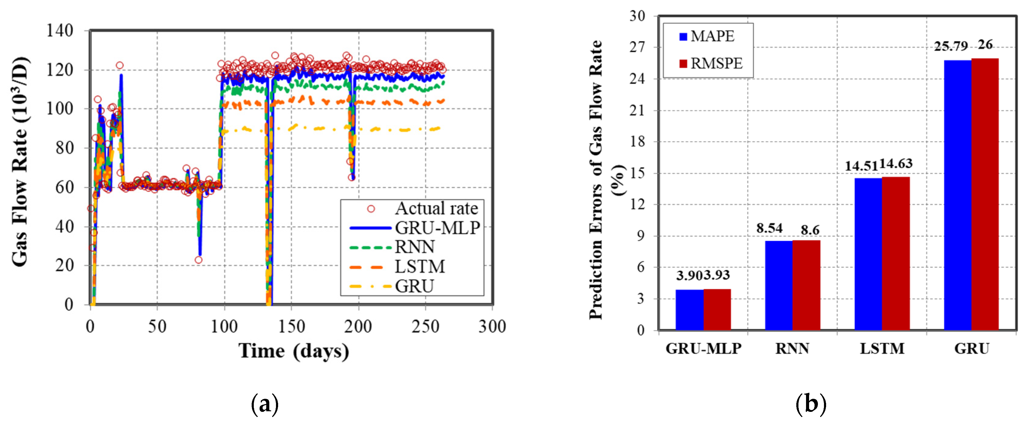
3.2.1. Error Comparisons

The GRU-MLP combined neural network is used for intelligent prediction because the model has better prediction accuracy than other single neural networks—for instance, GRU, LSTM, and RNN. The functions of the neural networks GRU and LSTM have been introduced above, but will not be explained in detail here. The history matching data and field data from the shale gas well were, respectively, imported into the four neural networks mentioned above to forecast production. Each model used one-half of the total data as training data and one-half as test data. Finally, four models were compared and the advantages of the GRU-MLP combined neural network were clarified compared with other single neural networks.
Figure 12a shows the results of shale gas production, as predicted by four neural network models, GRU-MLP, RNN, LSTM, and GRU. The predictions of the combined neural network model resulted as more consistent with historical production, while the GRU model showed the worst prediction results among the four models. The GRU-MLP model performed better in capturing the peak value of gas production. Figure 12b shows an error comparison between MAPE and RMSPE for the results obtained based on the four neural network models. The prediction error of the GRU-MLP model was significantly lower than other models. The MAPEs for shale gas production, generated by the RNN, LSTM, and GRU models, were 8.54%, 14.51%, and 25.79%, respectively. Models driven by data could learn the rule of production change, but they have difficulty in accurately predicting late-time production to match the real data due to the lack of sufficient physical constraints. Compared with the GRU model, which is driven by data, the GRU-MLP model performed well because it also used physical constraints. The MAPE and RMSPE of GRU-MLP model were 84.87% and 84.88% smaller than those of the GRU model, respectively. Therefore, a physics-constrained, data-driven method behaved better compared with a pure data-driven method. This indicates that the GRU-MLP model could be used to predict shale gas production precisely to provide invaluable references for decision makers regarding the optimization of completion parameters. Other data, such as fracture volume, total fluid volume, etc., can be incorporated into the model as physics constraints for more accurate predictions. It is possible to develop highly accurate models by response surface methodology and analysis of variance (ANOVA) using experimental and field data for prediction of various parameters during the production of shale reservoirs [45]. This can be a topic for future work.

3.2.2. CPU-Time Comparison

In addition to accuracy requirements, calculation efficiency is also a standard method of judging the applicability of the model. Table 3 shows the required time to forecast the production of the same shale gas well using numerical models and different neural network models. A comparison of central processing unit (CPU) time between different models is shown in Figure 13. The results obtained by time ratios (TX/TY) of different models were used for comparison. As shown in Figure 13, the time required by the neural network model was much less than that of the ordinary numerical simulation model, which illustrates that ML has a higher efficiency level in its capacity for shale gas production prediction. Meanwhile, it was observed that the GRU-MLP combined neural network model took slightly more time than the other three neural network models. The time was still within the acceptable range, because this combined neural network is more complex and accurate in processing procedures than other three models.

Limitations

The GRU-MLP model has no capability to automatically assess the importance of features. The gas–water two-phase numerical model analyzes the effect of fracture closure by considering the variation of conductivity with pressure and does not consider the variation of fracture geometry. The reservoir simulation and GRU-MLP model established herein are suitable for a single well, but not for the whole reservoir.

4. Conclusions

In this paper, we established a physical-constrained, data-driven model to predict shale gas production. EDFM and a numerical simulator were applied to generate data, while the GRU-MLP combined neural network model predicted the daily gas production. In addition, the NSGA II optimization algorithm was used to automatically optimize the model’s architecture. Missing the best model structure due to the researcher’s empirical decision was avoided. The result demonstrates that the workflow delivered high accuracy and efficiency in shale gas production forecasting. The major conclusions can be drawn as follows:
(1) The physics-constrained data-driven workflow is less dependent on field data than pure data-driven model. In shale gas production, there is inevitable uncertainty due to data from the subsurface. The physics-constrained data-driven workflow based on GRU-MLP is suitable for shale gas production prediction.
(2) The GRU-MLP model can predict multistage fractured horizontal shale gas well production efficiently and accurately. In addition, the model has a significant advantage in capturing the peak value of shale gas production. Compared to the RNN, LSTM, and GRU models, the GRU-MLP combined neural network model has a higher accuracy within an acceptable computational time range. GRU-MLP model generates MAPE and RMSPE values of 3.90% and 3.93%, respectively, which are 84.87% and 84.88% lower than those of the GRU model.
(3) RNN was incorporated into the workflow to analyze the contribution of each feature to the model, and initial hydraulic fracture conductivity made the greatest contribution to gas production within the features considered.
(4) There are still some limitations to our work. If microseismic data had been included in the model, the accuracy and efficiency of predicting production for naturally fractured reservoirs would have been improved.

Author Contributions

Methodology, formal analysis, X.Q.; resources, data curation, X.H.; visualization, investigation, H.L.; validation, W.S.; writing—original draft preparation, J.C. All authors have read and agreed to the published version of the manuscript.

Funding

This research was funded by A Physics-Constrained Data-Driven Method for Predicting Shale Oil/Gas Production Using Deep Learning Models (33550000-21-ZC0613-0326).

Data Availability Statement

No new data were created or analyzed in this study. Data sharing is not applicable to this article.

Acknowledgments

The authors would like to thank A Physics-Constrained Data-Driven Method for Predicting Shale Oil/Gas Production Using Deep Learning Models (33550000-21-ZC0613-0326) for financial support.

Conflicts of Interest

The authors declare no conflict of interest.

References

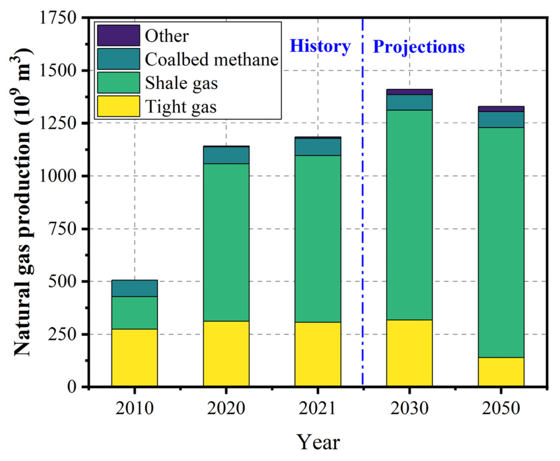
  1. Zou, C.; Xiong, B.; Xue, H.; Zheng, D.; Ge, Z.; Wang, Y.; Jiang, L.; Pan, S.; Wu, S. The role of new energy in carbon neutral. Petrol. Explor. Dev. 2021, 48, 480–491. [Google Scholar] [CrossRef]
  2. Yang, R.; Liu, X.; Yu, R.; Hu, Z.; Duan, X. Long short-term memory suggests a model for predicting shale gas production. Appl. Energ. 2022, 322, 119415. [Google Scholar] [CrossRef]
  3. IEA. World Energy Outlook 2022; IEA: Paris, France, 2022. [Google Scholar]
  4. Amorin, R.; Mensah, A. An Oil and Gas Retrofitted Carbon Capture Utilisation and Storage Value Chain: A Green Industry. J. Pet. Eng. Technol. 2022, 12, 10–18. [Google Scholar]
  5. Jukić, L.; Vulin, D.; Lukić, M.; Karasalihović Sedlar, D. Enhanced gas recovery and storability in a high CO2 content gas reservoir. Int. J. Greenh. Gas Con. 2022, 117, 103662. [Google Scholar] [CrossRef]
  6. Suriamin, F.; Ko, L.T. Chapter 2—Geological Characterization of Unconventional Shale-Gas Reservoirs. In Unconventional Shale Gas Development; Moghanloo, R.G., Ed.; Gulf Professional Publishing: Houston, TX, USA, 2022; pp. 33–70. [Google Scholar]
  7. Zhang, C.; Liu, S.; Ma, Z.; Ranjith, P. Combined micro-proppant and supercritical carbon dioxide (SC-CO2) fracturing in shale gas reservoirs: A review. Fuel 2021, 305, 121431. [Google Scholar] [CrossRef]
  8. Khormali, A.; Koochi, M.R.; Varfolomeev, M.A.; Ahmadi, S.J.J. Experimental study of the low salinity water injection process in the presence of scale inhibitor and various nanoparticles. Petrol. Explor. Dev. 2022, 13, 903–916. [Google Scholar] [CrossRef]
  9. Temizel, C.; Canbaz, C.; Aydin, H.; Wijaya, Z. A Deep Investigation of EOR/EGR and Stimulation Enhancement Methods in Unconventional Reservoirs. IOR 2021, 2021, 1–27. [Google Scholar]
  10. Wang, H.; Chen, L.; Qu, Z.; Yin, Y.; Kang, Q.; Yu, B.; Tao, W.-Q. Modeling of multi-scale transport phenomena in shale gas production—A critical review. Appl. Energ. 2020, 262, 114575. [Google Scholar] [CrossRef]
  11. Syed, F.I.; Muther, T.; Dahaghi, A.K.; Negahban, S. AI/ML assisted shale gas production performance evaluation. J. Pet. Explor. Prod. Technol. 2021, 11, 3509–3519. [Google Scholar] [CrossRef]
  12. Jiang, Z.; Wang, W.; Zhu, H.; Yin, Y.; Qu, Z. Review of Shale Gas Transport Prediction: Basic Theory, Numerical Simulation, Application of AI Methods, and Perspectives. Energy Fuels 2023, 37, 2520–2538. [Google Scholar] [CrossRef]
  13. Zhu, Q.; Lin, B.; Yang, G.; Wang, L.; Chen, M. Intelligent production optimization method for a low pressure and low productivity shale gas well. Petrol. Explor. Dev. 2022, 49, 886–894. [Google Scholar] [CrossRef]
  14. Koroteev, D.; Tekic, Z. Artificial intelligence in oil and gas upstream: Trends, challenges, and scenarios for the future. Energy AI 2021, 3, 100041. [Google Scholar] [CrossRef]
  15. Yang, R.Y.; Qin, X.Z.; Liu, W.; Huang, Z.W.; Shi, Y.; Pang, Z.Y.; Zhang, Y.Q.; Li, J.B.; Wang, T.Y. A Physics-Constrained Data-Driven Workflow for Predicting Coalbed Methane Well Production Using Artificial Neural Network. SPE J. 2022, 27, 1531–1552. [Google Scholar] [CrossRef]
  16. Vo Thanh, H.; Lee, K.-K. Application of machine learning to predict CO2 trapping performance in deep saline aquifers. Energy 2022, 239, 122457. [Google Scholar] [CrossRef]
  17. Vo Thanh, H.; Zamanyad, A.; Safaei-Farouji, M.; Ashraf, U.; Hemeng, Z. Application of hybrid artificial intelligent models to predict deliverability of underground natural gas storage sites. Renew Energy 2022, 200, 169–184. [Google Scholar] [CrossRef]
  18. Costa, L.A.N.; Maschio, C.; José Schiozer, D. Application of artificial neural networks in a history matching process. J. Petrol. Sci. Eng. 2014, 123, 30–45. [Google Scholar] [CrossRef]
  19. Wang, Q.; Jiang, F. Integrating linear and nonlinear forecasting techniques based on grey theory and artificial intelligence to forecast shale gas monthly production in Pennsylvania and Texas of the United States. Energy 2019, 178, 781–803. [Google Scholar] [CrossRef]
  20. Syed, F.I.; Alnaqbi, S.; Muther, T.; Dahaghi, A.K.; Negahban, S. Smart shale gas production performance analysis using machine learning applications. Pet. Res. 2022, 7, 21–31. [Google Scholar] [CrossRef]
  21. Nguyen-Le, V.; Shin, H. Artificial neural network prediction models for Montney shale gas production profile based on reservoir and fracture network parameters. Energy 2022, 244, 123150. [Google Scholar] [CrossRef]
  22. Niu, W.; Lu, J.; Sun, Y. Development of shale gas production prediction models based on machine learning using early data. Energy Rep. 2022, 8, 1229–1237. [Google Scholar] [CrossRef]
  23. Lee, K.; Lim, J.; Yoon, D.; Jung, H. Prediction of Shale-Gas Production at Duvernay Formation Using Deep-Learning Algorithm. SPE J. 2019, 24, 2423–2437. [Google Scholar] [CrossRef]
  24. Li, Y.; Sun, R.; Horne, R. Deep Learning for Well Data History Analysis. In Proceedings of the SPE Annual Technical Conference and Exhibition, Calgary, AB, Canada, 30 September 2019. [Google Scholar]
  25. He, Q.; Chen, J.-S. A physics-constrained data-driven approach based on locally convex reconstruction for noisy database. Comput. Methods Appl. Mech. Eng. 2020, 363, 112791. [Google Scholar] [CrossRef] [Green Version]
  26. Li, X.; Ma, X.; Xiao, F.; Xiao, C.; Wang, F.; Zhang, S. A physics-constrained long-term production prediction method for multiple fractured wells using deep learning. J. Petrol. Sci. Eng. 2022, 217, 110844. [Google Scholar] [CrossRef]
  27. Salehi, A.; Arslan, I.; Deng, L.; Darabi, H.; Smith, J.; Suicmez, S.; Castiñeira, D.; Gringarten, E. A Data-Driven Workflow for Identifying Optimum Horizontal Subsurface Targets. In Proceedings of the SPE Annual Technical Conference and Exhibition, 21–23 Paper presented at the SPE Annual Technical Conference and Exhibition, Dubai, United Arab Emirates, 21–23 September 2021. [Google Scholar]
  28. Park, J.; Datta-Gupta, A.; Singh, A.; Sankaran, S. Hybrid physics and data-driven modeling for unconventional field development and its application to US onshore basin. J. Petrol. Sci. Eng. 2021, 206, 109008. [Google Scholar] [CrossRef]
  29. Li, L.; Lee, S.H. Efficient Field-Scale Simulation of Black Oil in a Naturally Fractured Reservoir Through Discrete Fracture Networks and Homogenized Media. SPE Reserv. Eval. Eng. 2008, 11, 750–758. [Google Scholar] [CrossRef]
  30. Panfili, P.; Cominelli, A. Simulation of Miscible Gas Injection in a Fractured Carbonate Reservoir using an Embedded Discrete Fracture Model. In Proceedings of the Abu Dhabi International Petroleum Exhibition and Conference, Abu Dhabi, United Arab Emirates, 10–13 November 2014. [Google Scholar]
  31. Shakiba, M.; Sepehrnoori, K. Using Embedded Discrete Fracture Model (EDFM) and Microseismic Monitoring Data to Characterize the Complex Hydraulic Fracture Networks. In Proceedings of the SPE Annual Technical Conference and Exhibition, Houston, TX, USA, 28–30 September 2015. [Google Scholar]
  32. Shakiba, M.; de Araujo Cavalcante Filho, J.S.; Sepehrnoori, K. Using Embedded Discrete Fracture Model (EDFM) in numerical simulation of complex hydraulic fracture networks calibrated by microseismic monitoring data. J. Nat. Gas Sci. Eng. 2018, 55, 495–507. [Google Scholar] [CrossRef]
  33. Zeng, Q.-D.; Yao, J.; Shao, J. Study of hydraulic fracturing in an anisotropic poroelastic medium via a hybrid EDFM-XFEM approach. Comput. Geotech. 2019, 105, 51–68. [Google Scholar] [CrossRef]
  34. Xu, Y.; Cavalcante Filho, J.S.; Yu, W.; Sepehrnoori, K. Discrete-Fracture Modeling of Complex Hydraulic-Fracture Geometries in Reservoir Simulators. SPE Reserv. Eval. Eng. 2017, 20, 403–422. [Google Scholar] [CrossRef]
  35. Sun, J.; Ma, X.; Kazi, M. Comparison of Decline Curve Analysis DCA with Recursive Neural Networks RNN for Production Forecast of Multiple Wells. In Proceedings of the SPE Western Regional Meeting, Garden Grove, CA, USA, 22–27 April 2018. [Google Scholar]
  36. Li, X.; Ma, X.; Xiao, F.; Xiao, C.; Wang, F.; Zhang, S. Intelligence-Driven Prediction of Shear Wave Velocity Based on Gated Recurrent Unit Network. In Proceedings of the 56th U.S. Rock Mechanics/Geomechanics Symposium, Santa Fe, NM, USA, 26–29 June 2022. [Google Scholar]
  37. Olah, C. Understanding Lstm Networks. Available online: http://colah.github.io/posts/2015-08-Understanding-LSTMs/ (accessed on 27 August 2015).
  38. Siréta, F.-X.; Zhang, D. Smart Mooring Monitoring System for Line Break Detection from Motion Sensors. In Proceedings of the Thirteenth ISOPE Pacific/Asia Offshore Mechanics Symposium, Jeju, Republic of Korea, 14–17 October 2018. [Google Scholar]
  39. Gardner, M.W.; Dorling, S.R. Artificial neural networks (the multilayer perceptron)—A review of applications in the atmospheric sciences. Atmos. Environ. 1998, 32, 2627–2636. [Google Scholar] [CrossRef]
  40. Shi, Y.; Song, X.; Song, G. Productivity prediction of a multilateral-well geothermal system based on a long short-term memory and multi-layer perceptron combinational neural network. Appl. Energ. 2021, 282, 116046. [Google Scholar] [CrossRef]
  41. Yang, R.; Liu, W.; Qin, X.; Huang, Z.; Shi, Y.; Pang, Z.; Zhang, Y.; Li, J.; Wang, T. A physics-constrained data-driven workflow for predicting coalbed methane well production using a combined gated recurrent unit and multi-layer perception neural network model. In Proceedings of the SPE Annual Technical Conference and Exhibition, Dubai, United Arab Emirate, 21–23 September 2021. [Google Scholar]
  42. Nie, H.; Chen, Q.; Zhang, G.; Sun, C.; Wang, P.; Lu, Z. An overview of the characteristic of typical Wufeng–Longmaxi shale gas fields in the Sichuan Basin, China. NGIB 2021, 8, 217–230. [Google Scholar] [CrossRef]
  43. Yang, R.-Y.; Li, G.-S.; Qin, X.-Z.; Huang, Z.-W.; Li, J.-B.; Sheng, M.; Wang, B. Productivity enhancement in multilayered coalbed methane reservoirs by radial borehole fracturing. Pet. Sci. 2022, 19, 2844–2866. [Google Scholar] [CrossRef]
  44. Wang, T.; Tian, S.; Zhang, W.; Ren, W.; Li, G. Production model of a fractured horizontal well in shale gas reservoirs. Energ. Fuel 2020, 35, 493–500. [Google Scholar] [CrossRef]
  45. Ahmadi, S.; Khormali, A.; Khoutoriansky, F.M. Optimization of the demulsification of water-in-heavy crude oil emulsions using response surface methodology. Fuel 2022, 323, 124270. [Google Scholar] [CrossRef]
Figure 1. World unconventional natural gas production and forecast [3].
Processes 11 00806 g001
Figure 2. The schematic of GRU [37].
Processes 11 00806 g002
Figure 3. Schematic of a GRU-MLP combined neural network [15].
Processes 11 00806 g003
Figure 4. Workflow based on the GRU-MLP model.
Processes 11 00806 g004
Figure 5. Schematic of the geometric model for numerical reservoir simulation and curves of the field data: (a) geometric model; (b) field data.
Processes 11 00806 g005
Figure 6. Production with different hydraulic fracture half-lengths: (a) gas flow rate; (b) cumulative gas production.
Processes 11 00806 g006
Figure 7. Production with different initial hydraulic fracture conductivity values: (a) gas flow rate; (b) cumulative gas production.
Processes 11 00806 g007
Figure 8. Production with different natural fracture numbers: (a) gas flow rate; (b) cumulative gas production.
Processes 11 00806 g008
Figure 9. Production with different natural fracture conductivity values: (a) gas flow rate; (b) cumulative gas production.
Processes 11 00806 g009
Figure 10. Production with different natural fracture conductivity values.
Processes 11 00806 g010
Figure 11. Comparison of model simulation and field data: (a) gas flow rate; (b) cumulative gas production; (c) water flow rate; (d) cumulative water production; (e) bottom hole pressure; (f) pressure distribution after 305 days of production.
Processes 11 00806 g011aProcesses 11 00806 g011b
Figure 12. Comparisons of four neural network models: (a) daily gas production prediction; (b) prediction errors.
Processes 11 00806 g012
Figure 13. CPU time comparison between different models.
Processes 11 00806 g013
Table 1. Parameters values for sensitivity studies.
ParameterValueUnit
Hydraulic fracture properties
Hydraulic fracture half-length75, 100, 125, 150m
Initial hydraulic fracture conductivity10, 25, 50, 75mD·m
Natural fractures properties
Natural fracture number250, 500, 750, 1000-
Initial natural fracture conductivity0.01, 0.1, 1 3mD·m
Table 2. Basic reservoir model parameters.
ParameterValueUnit
Reservoir properties
Model dimensions [L × W × H]1500 × 400 × 30m
Reservoir temperature 80°C
Reservoir depth3000m
Initial reservoir pressure35MPa
Matrix permeability0.0009mD
Matrix porosity0.08%
Reservoir thickness30m
Initial water saturation35%
Hydraulic fracture properties
Hydraulic fracture number20-
Hydraulic fracture spacing50m
Hydraulic fracture half-length100m
Hydraulic fracture width0.025m
Initial hydraulic fracture conductivity10mD·m
Natural fracture properties
Natural fracture number800-
Natural fracture width0.001m
Initial natural fracture conductivity3.5mD·m
Well parameters
Wellbore diameter0.057m
Horizontal length600m
Table 3. The CPU times of different models for gas flow rate.
Numerical
Model(s)
GRU-MLP(s)GRU(s)LSTM(s)RNN(s)
Gas107.78.648.256.287.47
Disclaimer/Publisher’s Note: The statements, opinions and data contained in all publications are solely those of the individual author(s) and contributor(s) and not of MDPI and/or the editor(s). MDPI and/or the editor(s) disclaim responsibility for any injury to people or property resulting from any ideas, methods, instructions or products referred to in the content.

