Article

A Knowledge-Based Cooperative Differential Evolution Algorithm for Energy-Efficient Distributed Hybrid Flow-Shop Rescheduling Problem

1
School of Information Science and Engineering, Harbin Institute of Technology, Weihai 264209, China
2
College of Metrology & Measurement Engineering, China Jiliang University, Hangzhou 310018, China
*
Author to whom correspondence should be addressed.
Processes 2023, 11(3), 755; https://doi.org/10.3390/pr11030755
Submission received: 5 February 2023 / Revised: 25 February 2023 / Accepted: 28 February 2023 / Published: 3 March 2023

Abstract

:
Due to the increasing level of customization and globalization of competition, rescheduling for distributed manufacturing is receiving more attention. In the meantime, environmentally friendly production is becoming a force to be reckoned with in intelligent manufacturing industries. In this paper, the energy-efficient distributed hybrid flow-shop rescheduling problem (EDHFRP) is addressed and a knowledge-based cooperative differential evolution (KCDE) algorithm is proposed to minimize the makespan of both original and newly arrived orders and total energy consumption (simultaneously). First, two heuristics were designed and used cooperatively for initialization. Next, a three-dimensional knowledge base was employed to record the information carried out by elite individuals. A novel DE with three different mutation strategies is proposed to generate the offspring. A local intensification strategy was used for further enhancement of the exploitation ability. The effects of major parameters were investigated and extensive experiments were carried out. The numerical results prove the effectiveness of each specially-designed strategy, while the comparisons with four existing algorithms demonstrate the efficiency of KCDE in solving EDHFRP.

1. Introduction

Productivity has become one of the core competencies in the manufacturing industry, particularly with the integration of the world economy. However, with the ongoing trend of mass customization and the accelerated variety of products, a growing number of manufacturing companies have realized the importance of environmentally friendly manufacturing. As the most energy-consuming and CO 2 emission entity, China’s energy structure highly depends on coal. More than half of the electrical production is fueled by coal, while over 70% of power plants are coal-fired [1]. Energy-efficient scheduling of manufacturing industries is an effective way to reduce carbon emissions [2]. Therefore, it is of extraordinary significance to develop production schedules for intelligent manufacturing industries with energy-related constraints and objectives.
By extending the production model into the distributed environment and establishing multiple factories in various remote geographical locations, distributed manufacturing has been widely applied in various fields, including automotive, steel-making, and chemical processing [3]. In the past few decades, various evolutionary algorithms, such as artificial bee colony [4], iterated greedy algorithm [5], Jaya algorithm [6], and memetic algorithm [7], have been proposed to solve distributed shop scheduling problems with different constraints. The authors of [8] focused on the distributed parallel machine-scheduling problem and proposed a knowledge-based two-population optimization algorithm to minimize the energy consumption and total tardiness simultaneously. A distributed flow-shop group scheduling problem was investigated and solved by a cooperative co-evolutionary algorithm with a novel collaboration model and a reinitialization scheme in [9]. The authors of [10] studied a distributed heterogeneous hybrid flow-shop scheduling problem (FSP) under nonidentical time-of-use electricity tariffs, of which, the makespan and total electricity charges were considered as optimization objectives. Distributed hybrid differentiation FSP was investigated in [11], for which a distributed co-evolutionary memetic algorithm was proposed to minimize the makespan. Recently, the combination of distributed flow-shop and parallel machines, namely the distributed hybrid flow-shop scheduling problem (DHFSP), has emerged as a practical production model. In order to provide an efficient productive schedule for DHFSP, ref. [7] proposed a bi-population cooperative memetic algorithm. For energy-aware DHFSP with multiprocessor tasks, [12] proposed a multi-objective evolutionary algorithm based on decomposition while [13] designed a knowledge-based multi-objective algorithm.
Uncertainties always exist in real-life manufacturing. Unlike determinate processing, rescheduling aims to make schedules under dynamic environments, dealing with unpredicted events, such as new job arrivals and machine breakdowns. Rescheduling in FSP with variable processing times by using real-time information was studied in [14]. Rescheduling jobs in flexible job-shop scheduling problem (FJSP) is receiving more attention. FJSP (with newly arrived priority jobs) was investigated in [15], while machine breakdowns and FJSP recovery were considered in [16,17]. The authors of [18,19] took both real-time order acceptance and machine maintenance into consideration when rescheduling the FJSP. Furthermore, [20] provided energy-efficient schedules for FJSP with dynamic variations occurring frequently during production. The authors of [21] focused on rescheduling for the hybrid flow-shop scheduling problem (HFSP), in which energy consumption was regarded as an objective and the real-time order acceptance was considered. Moreover, [22] focused on steelmaking systems and proposed a hybrid fruit fly optimization algorithm to solve the rescheduling problem in HFSP with machine breakdowns and processing variations, while the release variation was considered in [23]. Moreover, rescheduling for a single-machine problem was studied in [24], in which the total waiting time was set as an objective and the newly arrived reworked jobs were considered. Rescheduling (in several identical parallel-machine problems) was investigated in [25]; the sequence-dependent setup times, release times, and newly arrived jobs were considered.
Inspired by the natural evolution of species, differential evolution (DE) is a simple (yet efficient) heuristic for global optimization over continuous spaces [26]; it has been improved in the past few decades and widely applied as a state-of-the-art global optimization technique in a variety of scheduling problems [27]. In [28], DE was combined with a local search mechanism to minimize the makespan and tardiness of FSP simultaneously. In order to solve permutation FSP while minimizing the makespan, optimization algorithms based on discrete DE were designed in [29], and a DE with the algebraic differential mutation was designed in [30], considering the total flowtime criterion. Time-of-use electricity tariffs were considered in [31], where a multi-objective discrete DE with novel mutations and crossover operations was developed. The authors of [32] combined DE with heuristic strategies in order to solve FJSP with outsourcing operations and job priority constraints, while a new mutation strategy based on searching was designed for DE in [33] to minimize the makespan in FJSP with reconfigurable machine tools. Moreover, DE was used for scheduling hybrid FSP [34] and JSP with fuzzy processing times [35,36]. In [8], DE performed cooperatively with NSGA-II on the population in parallel and provided efficient solutions for the distributed energy-efficient parallel machine-scheduling problem. Moreover, DE is used for solving other scheduling problems, such as robotic cell scheduling with batch-processing machines [37] and a single batch-processing machine with arbitrary job sizes and release times [38].
This study aims to solve the energy-efficient distributed hybrid flow-shop rescheduling problem (EDHFRP) by minimizing the makespan of both the first-order and the newly arrived order, along with the total energy consumption. EDHFRP can be considered as an extension of the existing DHFSP, which is studied in [7,12], by adding constraints, including energy-efficient and newly-arrived jobs. The mathematical model of EDHFRP is provided in Section 2.1, appending the calculation of energy consumption and the description of rescheduling on the basis of the model of DHFSP defined in [7,12]. In order to solve this problem, a knowledge-based cooperative differential evolution (KCDE) algorithm is proposed. In KCDE, two heuristics are designed for initialization according to the characteristics of EDHFRP. Then, a three-dimensional knowledge base is proposed to describe the information carried out by elite individuals. Moreover, three novel differential mutation strategies along with a crossover method are employed to the knowledge base for evolution. Additionally, a local intensification strategy was designed for elite individuals in order to further improve the quality of solutions. Finally, extensive comparisons and tests were carried out to verify the efficiency and effectiveness of the proposed KCDE in solving EDHFRP.
The remainder of this paper is divided into four parts. Section 2 describes EDHFRP in detail and provides the mathematical model. Every strategy and design of KCDE is introduced in Section 3. The numerical results and discussion are shown in Section 4. Finally, the conclusion provides a brief summary and critique of the findings in Section 5.

2. Distributed Hybrid Flow-Shop Rescheduling Problem

2.1. Problem Description

The indices, parameters, variables and decision variables used in the following description is shown as follows.
IndicesDescription
FNumber of factories.
fIndex of factories, f { 1 , 2 , , F } .
O 1 The first order.
O 2 The newly arrived order during the processing of O 1 .
n 1 Number of jobs in O 1 .
n 2 Number of jobs in O 2 .
n p Number of jobs under processing at time t a in O 1 .
n u Number of unprocessed jobs at time t a in O 1 .
j 1 Index of jobs in O 1 , j 1 { 1 , 2 , , n 1 } .
j 2 Index of jobs in O 2 , j 2 { 1 , 2 , , n 2 } .
j p Index of jobs under processing at time t a , j p { 1 , 2 , , n p } .
j u Index of unprocessed jobs at time t a , j u { 1 , 2 , , n u } .
jIndex of all jobs, j { 1 , 2 , , n 1 + n 2 } .
sNumber of stages.
kIndex of stages, k { 1 , 2 , , s } .
m f , k Number of machines for stage k in factory f.
iIndex of machines, i { 1 , 2 , , m f , k } .
ParametersDescription
t a The arrival time of O 2 .
P j , k Processing time of job j at stage k.
E P f , k , i Energy consumption of machine i per unit time at stage k in factory f in
processing mode.
E I Energy consumption per unit time in idle mode.
VariablesDescription
E C P f , k , i Energy consumption of machine i in processing mode at stage k in factory f.
E C I f , k , i Energy consumption of machine i in idle mode at stage k in factory f.
S j , k Begin time of processing job j at stage k.
C j , k Completion time of processing job j at stage k.
M S 1 Makespan of O 1 .
M S 2 Makespan of O 2 .
T E C Total energy consumption.
Decision VariablesDescription
x j , f Binary variable whose value equals 1 when job j is assigned to
factory f or 0 otherwise.
y j , f , k , i Binary variable whose value equals 1 when job j is assigned to
machine i at stage k in factory f or 0 otherwise.
z j , j , f , k , i Binary variable whose value equals 1 when job j is processed
before j on machine i at stage k in factory f or 0 otherwise.
In a typical DHFSP, the total number of n jobs need to be processed on a set of machines. Each job includes s stages and there are one or more machines for each stage. Moreover, the machines belong to F-geographically dispersed factories. Each job needs to be assigned to one of the factories before processing, and should not be removed from the certain factory until completion. Therefore, in order to schedule DHFSP, three sub-problems demand solving, namely factory assignment, machine selection, and job sequencing.
In EDHFRP, during the processing of n 1 jobs in the first-order O 1 , another order O 2 with n 2 jobs arrives at time t a and needs to be completed as soon as possible. At time t a , the possible states of jobs in O 1 are completed, under processing, and unprocessed. For jobs in the first two states, the original schedule is kept, while the unprocessed jobs in O 1 need rescheduling along with the new jobs in O 2 . However, during the rescheduling, the available time of each machine changes from 0 to the completion time of jobs under processing at time t a . Furthermore, the unprocessed jobs in O 1 have to remain in the factories to which they are assigned, while the newly arrived jobs in O 2 can be assigned to any factory. Therefore, the complexity of scheduling EDHFRP is much higher than the typical DHFSP.
The Gantt chart of a solution of an instance with n 1 = 8 , n 2 = 5 , s = 3 , F = 2 , and t a = 30 is illustrated in Figure 1. The original schedule for O 1 is shown in Figure 1a; it can be seen that job 1 and job 7 in factory 1, as well as job 8 in factory 2 are unprocessed when new order O 2 arrives at t a . Thus, the three unprocessed jobs along with jobs in O 2 are rescheduled, while job 1 and job 7 still remain in factory 1 and job 8 in factory 2. The processing plan after rescheduling is shown in Figure 1b, in which the rectangles labeled II-1∼II-5 denote the jobs in O 2 . The makespan of O 1 and O 2 are 163 and 195 min, respectively, and the total energy consumption can be calculated as 134.08 kJ.

2.2. Mathematical Model

The mixed integer linear programming model for EDHFRP minimizing M S 1 , M S 2 and T E C is formulated as follows:
min ( M S 1 , M S 2 , T E C )
Subject to:
f = 1 F x j , f = 1     j
i = 1 m f , k y j , f , k , i = 1     f , j , k
S j 1 , 1 0     j 1
n p + n u = n 1
C j , k = S j , k + P j , k     j , k
S j , k + 1 C j , k     j   k { 1 , 2 , , s 1 }
z j , j , f , k , i + z j , j , f , k , i 1     j j , f , k , i { 1 , 2 , , m f , k }
z j , j , f , k , i + z j , j , f , k , i y j , f , k , i + y j , f , k , i 1     j j , f , k , i
S j , k C j , k + 10 6 × ( 3 y j , f , k , i y j , f , k , i z j , j , f , k , i ) 0     j j , f , k , i
M S 1 C j 1 , s     j 1
M S 2 C j 2 , s     j 2
E C P f , k , i = j = 1 n y j , f , k , i × E P f , k , i × P j , k     f , k , i { 1 , 2 , , m f , k }
E C I f , k , i = E I × [ max j ( C j , k × y j , f , k , i ) min j ( S j , k + 1 × y j , f , k , i ) j = 1 n y j , f , k , i × P j , k ] f , k , i { 1 , 2 , , m f , k }
T E C = f = 1 F k = 1 s i = 1 m f , k ( E C P f , k , i + E C I f , k , i )
x j , f { 0 , 1 }   j , f
y j , f , k , i { 0 , 1 }   j , f , k , i { 1 , 2 , , m f , k }
z j , j , f , k , i { 0 , 1 }   j , j , f , k , i
where Equation (1) describes the three optimization objectives, Equation (2) assures that only one factory must be selected for each job, Equation (3) ensures that the processing of each stage of each job must happen on only one machine, Equation (4) guarantees all jobs in O 1 must be processed after time 0, Equation (5) makes sure that each job in O 1 is either under-processed or unprocessed at time t a , Equation (6) defines the calculation of the completion time, Equation (7) ensures that each stage can only be processed after the completion of the previous one, Equations (8)–(10) guarantee that each machine can process—at most—one job at any time, Equations (11)–(12) define the makespan of two orders, Equations (13)–(15) calculate the total energy consumption. Equations (16)–(18) indicate the binary decision variables.

3. KCDE for EDHFRP

The classical DE refers to an efficient and powerful population-based stochastic search technique for solving optimization problems over a continuous space, aiming to evolve a population of D-dimensional parameter vectors, which encode the candidate solutions toward the global optimum. However, as a discrete optimization problem, the parameter vectors built for job-shop scheduling problems are limited to being positive integers according to the constraints; thus, it is difficult for DE to reach its full potential when directly used in solving job-shop scheduling problems. The knowledge base proposed in this paper is capable of making an explicit connection between continuous space and discrete parameter vectors. In this section, the representation of the solution is first introduced briefly, following by the details of four vital components of KCDE, including hybrid initialization, knowledge base, cooperative differential mutation, and local intensification.

3.1. Solution Representation

For each job in EDHFRP, the factory assignment should be determined first, then a machine is selected for each stage, while the processing sequence on each machine should be determined at the same time. In this paper, the efficient and widely used permutation-encoding method is employed to represent the job sequence in each factory. Machine assignments are obtained through decoding operations according to the job sequence and factory assignment. Therefore, the solutions of EDHFRP can be encoded as { N 1 , , N F , Π 1 , , Π F } , where N f , f { 1 , 2 , , F } denotes the number of jobs assigned to factories f, Π f , f { 1 , 2 , , F } represents the processing sequence of jobs at the first stage in factory f. Considering the feasibility of the solutions, each job should occur in the job sequence of any factory once and only once.
To be specific, the corresponding solution of the Gantt chart in Figure 1a—before new order arrival—is shown in Figure 2a, from which it can be seen that jobs 3, 5, 7, and 1 are processed in factory 1 sequentially, while the first job processed in factory 2 is job 4, followed by jobs 2, 6, and 8. When O 2 arrives at time t a , jobs 3, 5, 4, and 2 are being processed, while jobs 7, 1, 6, and 8 remain unprocessed. Therefore, the 4 unprocessed jobs along with the 5 new jobs are rescheduled as in Figure 2b, in which jobs 7, 1, 6, and 8 are still in the factories they were assigned to at first.

3.2. Hybrid Initialization

In order to strike a balance between the quality and variety of the initial population, three different initialization strategies, including two EDHFRP characteristic-based heuristics and a random method, were designed and employed in a cooperative manner.
It has been conclusively shown that the Nawaz–Enscore–Ham (NEH) heuristic [39] is one of the most effective heuristics for solving FSP [40]. Recently, the variants of NEH heuristics have been widely used in DFSP and DHFSP [5,6,41,42]. In this paper, a greedy NEH heuristic (GNEH) and a NEH heuristic based on lower bounds (NEHLB) are proposed.
For both heuristics, the initial job sequences are generated randomly and the jobs are arranged sequentially. The main method of GNEH is described as Algorithm 1 in detail. First, each job is inserted into all possible position in each factories. Next, the values of M S 1 and T E C of each insertion are calculated. Then, the insertion with the best result is selected. Moreover, N P / 3 individuals are generated through GNEH.
Algorithm 1: Greedy NEH heuristic
Processes 11 00755 i001
The NEHLB is designed as Algorithm 2 and implemented to generate N P / 3 individuals. For each job, the current L B M S 1 and L B T E C of each factory are calculated first. Next, the factory with the smallest value is chosen. Then, the job is inserted into one of the possible positions in a certain factory (randomly). In order to increase the diversity of the initial population, the rest of the population is generated randomly.
Algorithm 2: NEH heuristic with biased optimization
Processes 11 00755 i002

3.3. 3D Knowledge Base

Taking the features of DE and EDHFRP into consideration, a three-dimensional knowledge base is designed to store the information of elite individuals. In the proposed knowledge base, both x-axis and y-axis represent the jobs, while the z-axis represents the factories. Therefore, the x y -plane is a square, whose side lengths are equal to the number of jobs n. The value of the knowledge base at position ( x 0 , y 0 , z 0 ) , where x 0 , y 0 1 , 2 , , n , x 0 y 0 and z 0 { 1 , 2 , , F } , denotes the probability that both job x 0 and y 0 are assigned to the same factory z 0 while job x 0 is processed before job y 0 , while the value of position ( x 0 , x 0 , z 0 ) means the probability that job x 0 is assigned to factory z 0 .
The knowledge base is initialized as Equation (19), where j 1 , j 2 { 1 , 2 , , n 1 } and f { 1 , 2 , , F } .
K B 0 ( j 1 , j 2 , f ) = 0.5 ,   if   j 1 j 2 1 ,   if   j 1 = j 2
At the end of each generation, the knowledge base is updated according to the non-dominated solutions. For each elite individual p o p e in E ( g ) , e 1 , 2 , , n E , an incremental matrix δ e is calculated according to Equations (20) and (21) where j 1 , j 2 { 1 , 2 , , n F } , j 1 j 2 , and n E is the number of non-dominated solutions.
δ e ( j 1 , j 2 , f ) = 1 ,   if   j 1   is   processed   before   j 2   in   factory   f 0 ,   otherwise
δ e ( j , j , f ) = 1 ,   if   j   is   assigned   to   factory   f 0 ,   otherwise
Finally, the knowledge base is updated via Equation (22) and normalized as Equation (23).
K B g = ( 1 α ) × K B g 1 + α × e = 1 n E δ e n E
K B g ( x , y , z ) = K B g ( x , y , z ) z = 1 F K B ( x , y , z ) ,   if   x = y K B g ( x , y , z ) x = 1 n y = 1 n K B ( x , y , z ) ,   if   x y
Through the operations above, the useful information of better-performed solutions is transformed from the discrete model into the continuous space, which is more suitable to work DE to its advantage. Moreover, the processing priority between different jobs and the information of the factory assignment are linked together.

3.4. Cooperative DE

As the most important step of DE, the mutation operator provides new individuals for the population and considerable research studies have proposed modifications in mutation strategies in the past two decades [43]. A total of six most popular types of mutation operators of DE and their characteristics are represented in [44]. As a result of the performance insufficiency of each single mutation strategy, the cooperation among several different strategies has been used to solve complicated scheduling problems [33,45,46]. Since the mutation operator DE/rand/1 has the most exploration properties but very limited exploitation abilities, DE/best/1 has the most exploitation ability but may end up in premature convergence, while DE/current-to-best/1 has both the exploration and exploitation properties according to its utilization of the memory set of individuals, the cooperation among them may avoid being trapped in local optima and ensure the balance between the diversification and intensification when searching for the optimal solution. In this paper, three differential mutation strategies, i.e., DE/rand/1, DE/best/1, and DE/current-to-best/1, are used cooperatively with the knowledge base according to the weight vector w = [ w 1 , w 2 , w 3 ] . The main method of cooperative DE is shown in Algorithm 3. The individuals for each DE strategy are calculated as N P 1 = round ( N P × w 1 ) , N P 2 = round ( N P × w 2 ) , and N P 3 = N P N P 1 N P 2 .
Algorithm 3: Cooperative Differential Evolution
Processes 11 00755 i003

3.4.1. Mutation

For each individual in P o p 1 ( g ) , the DE/rand/1 strategy is carried out on K B g , for which three individuals are selected from P o p 1 ( g ) randomly. Next, the best of them is recorded as x r 0 according to the non-dominated sort, while the worst individual is named x r 2 , and the rest are denoted as x r 1 . Then, a variant matrix can be obtained through differential mutation, as described in Equations (24) and (25), where x , y { 1 , 2 , , n } , x y , z { 1 , 2 , , F } and F m denote the mutation factors.
Δ 1 ( x , y , z ) = 1 ,   if   job   x   is   processed   before   job   y   in   factory   z   in   x r 0 F m ,   if   job   x   is   processed   before   job   y   in   factory   z   in   x r 1 F m ,   if   job   x   is   processed   before job   y   in   factory   z   in   x r 2
Δ 1 ( x , x , z ) = 1 ,   if   job   x   is   assigned   to   factory   z   in   x r 0 F m ,   if   job   x   is   assigned   to   factory   z   in   x r 1 F m ,   if   job   x   is   assigned   to   factory   z   in   x r 2
The DE/best/1 strategy is carried out on K B g for each individual in P o p 2 ( g ) . A total of three individuals, including the best one in P o p 2 ( g ) and two other ones randomly selected, are selected and denoted as x b e s t , x r 1 and x r 2 . Then, the differential mutation is carried out as Equations (24) and (25), in which the x r 0 is replaced by x b e s t , thus the variant matrix Δ 2 is received.
As for the DE/current-to-best/1, the current individual along with the best one in P o p 3 ( g ) and two randomly selected ones are chosen and recorded as x i , x b e s t , x r 1 and x r 2 respectively. Then, the variant matrix is generated through Equations (26) and (27).
Δ 3 ( x , y , z ) = 2 × F m ,   if   job   x   is   processed   before   job   y   in   factory   z   in   x b e s t 1 2 × F m ,   if   job   x   is   processed   before   job   y   in   factory   z   in   x i F m ,   if   job   x   is   processed   before   job   y   in   factory   z   in   x r 1 F m ,   if   job   x   is   processed   before   job   y   in   factory   z   in   x r 2
Δ 3 ( x , x , z ) = 2 × F m ,   if   job   x   is   assigned   to   factory   z   in   x b e s t 1 2 × F m ,   if   job   x   is   assigned   to   factory   z   in   x i F m ,   if   job   x   is   assigned   to   factory   z   in   x r 1 F m ,   if   job   x   is   assigned   to   factory   z   in   x r 2

3.4.2. Crossover

The crossover operator constructs a new trial individual under the guidance of a target individual and a mutant individual [43]. Most of the existing crossover operators of DE are binomial variant, which is essentially suitable for solving continuous optimization problems. However, as a discrete problem, job-shop scheduling problems have various limits on structuring individuals. Most of the existing research using DE to solve scheduling problems have paid attention to the modification of crossover strategies or the structure of individuals instead of alteration in both of them [47], which may cause mismatching between the problem and the algorithm. Thus, on the basis of the knowledge base, a problem-specific crossover operator is proposed as follows.
With Δ d and K B g , an offspring matrix can be obtained through crossover, which is shown in Equation (28).
K B g d = ( 1 C R ) × K B g + C R × Δ d
where C R is the crossover probability, Δ d , d { 1 , 2 , 3 } indicates the three variant matrices provided by three DE strategies, and K B g d is the corresponding offspring matrix.
Finally, an offspring individual is sampled from K B g 1 according to the Roulette wheel selection strategy. The sampling operation mainly consists of two steps, choosing the factory for every job and sorting the jobs in each factory. In the first step, the certain factory f with max f K B g d ( j , j , f ) is selected for each job j. Then, jobs assigned to the same factory are chosen one by one via the roulette wheel selection strategy according to the value of K B g d ( j , j , f ) ; thus, jobs with higher values are more likely to be processed earlier.

3.4.3. Selection

The offspring generated through DE/rand/1, DE/best/1, and DE/current-to-best/1, denoted as P o p N e w 1 ( g ) , P o p N e w 2 ( g ) , and P o p N e w 3 ( g ) , respectively, are gathered together as P o p N e w ( g ) , with a size of N P . Next, the newly generated population P o p N e w ( g ) and the current population P o p ( g ) are united and the best N P individuals are selected according to non-dominated sorting. During the selection, the chosen individuals belonging to P o p N e w 1 ( g ) , P o p N e w 2 ( g ) , and P o p N e w 3 ( g ) are recorded as N u m 1 , N u m 2 , and N u m 3 , respectively. Then, the weight vector is updated as Equation (29).
w = [ N u m 1 N u m 1 + N u m 2 + N u m 3 , N u m 2 N u m 1 + N u m 2 + N u m 3 , N u m 3 N u m 1 + N u m 2 + N u m 3 ]
According to the descriptions of the three DE strategies, the minimum number of individuals for each group is four. In order to guarantee the feasibility of the cooperative DE, the lower bound of w 1 , w 2 , and w 3 in the weight vector is set as 0.1. In other words, the value of elements in w smaller than 0.1 will be improved to 0.1, while the other elements will be decreased in proportion.

3.5. Local Intensification

In order to further enhance the quality of solutions, a local intensification is designed and carried out on non-dominated individuals at the end of each generation. The main method of local intensification is described in Algorithm 4. For each non-dominated individual, the factories with the maximum and minimum completion times are first selected, denoted as the critical factory f c and the easiest factory f e , respectively. Next, a job assigned to f c is chosen randomly, which is then inserted into all possible positions in f e . After that, the objective values of each insertion are calculated and the best one is kept as a neighbor. Finally, the N P best individuals are selected from the union of the current population and neighbors.
Algorithm 4: Local intensification
Processes 11 00755 i004

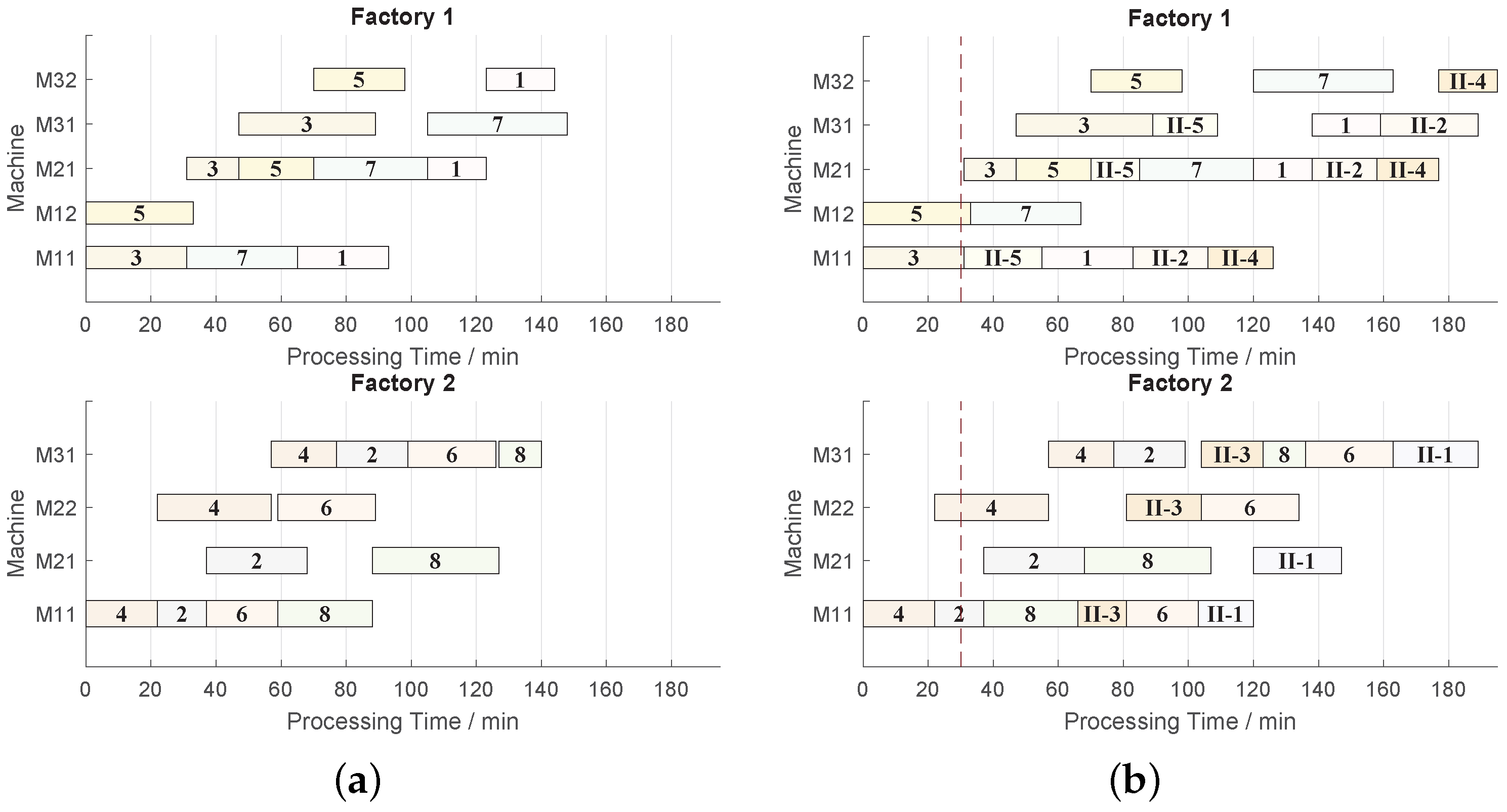
3.6. Rescheduling Strategy

When the new order O 2 arrives, the following tasks are completed before carrying out the KCDE.
  • The state of jobs in O 1 at time t a are recorded, and the unprocessed jobs are counted.
  • The unprocessed jobs are then put with jobs in O 2 , together forming the new order. The factory assignments of unprocessed jobs are also recorded, which are used as the constraints during the rescheduling stage since the jobs cannot be transformed into other factories once assigned.
  • The available machine times are updated into the completion times of jobs, which are processed at time t a .

3.7. Framework of KCDE

The framework of the proposed KCDE is depicted in Figure 3. Three differential evolution strategies are employed cooperatively on the knowledge base, and a self-adaptive weight vector is designed to control the proportion of the application of three strategies according to the quality of the offspring generated by them. Moreover, several problem-specific strategies, such as hybrid initialization, update of the knowledge base, and local intensification, are implemented. The performance of such a properly designed algorithm in solving EDHFRP is highly expected.

4. Numerical Results and Comparisons

4.1. Experimental Settings

A considerable amount of instances are generated and employed to test the performance of KCDE in solving EDHFRP. Each instance has four decisive factors for its scale, including the number of factories F, the number of jobs in the first order n 1 , the number of jobs in the new order n 2 , and the number of stages s. In this paper, the value of F is collected from { 3 , 4 , 5 } , the value of n 1 is from { 30 , 50 , 80 } , while n 2 is selected from { 20 , 30 , 50 } and s is from { 4 , 5 , 6 } . Moreover, the processing time and energy consumption of the per-unit time is sampled from the instances provided by early research for similar problems [12,41]. Moreover, 10 instances are generated for each combination of F, n 1 , n 2 , and s; thus, a total of 3 × 3 × 3 × 3 = 81 instances in 81 different scales are used in the following tests and comparisons. The arrival time of O 2 is set randomly, while instances with the same scales own the same t a .
Generally, more running time is needed in each iteration for a scheduling instance with higher complexity, while the operation is faster when it comes to an easy instance. In order to guarantee the reasonableness and fairness of the experiments on instances with different scales, the maximum running time is set according to the four decisive factors for the scale. [d=R1.]Therefore, for Foreach compared algorithm and testing algorithm, the maximum running time for the first order is set as 0.1 × F × n 1 × s seconds, while it is set as 0.1 × F × n 2 × s seconds after O 2 ’s arrival. To be fair, all algorithms were implemented through MATLAB2021b and conducted in the same computer environment with 12th Gen Intel Core i7-12700K, 3.61GHz, 32GB RAM, and Windows 10 OS.
Three commonly used metrics in the multi-optimization field, i.e., hyper-volume (HV), C metric (CM), and generational distance (GD) [48] are utilized to evaluate the performance of the algorithms, which focus on measuring the convergence and diversity of the Pareto set approximations.

4.2. Model Validation

In order to validate the mathematical model provided in Section 2.2, 10 small-scale instances are generated randomly, and the exact solver IBM ILOG CPLEX 12.9 is used to compare with the proposed algorithm. For each comparison, both CPLEX and KCDE run 10 times independently. In each run, the CPU time limit of CPLEX is set to 1 h while the stopping criterion of KCDE is set as mentioned above. Since the rescheduling solution is obtained on the basis of the schedule of the original order, and depends on the producing state at time t a , the comparison on each instance is divided into two parts.
In the first part, the original schedule O 1 is scheduled by both CPLEX and KCDE, the results ( M S 1 and T E C ) are compared. In the second part, the scheduling plan of the original order obtained by CPLEX is used for both the solver and the algorithm to solve the rescheduling problem; the results M S 1 , M S 2 , and T E C are compared again.
The results of the first comparison are shown in the left column of Table 1, from which it can be seen that small differences exist between the results obtained by CPLEX and KCDE, while KCDE achieves most of the better results. The right column in Table 1 provides the results of the second comparison, in which the objective values given by KCDE are better than those provided by CPLEX in all instances. Therefore, the mathematical model of EDHFRP is validated.

4.3. Parameter Setting

There exist three important parameters in the proposed KCDE: (1) the mutation factor in the differential mutation operation ( F ) , (2) the probability of crossover in DE ( C R ) , (3) and the weight factor used for updating the knowledge base ( α ) . In order to inspect the effects of these parameters on the performance of KCDE and choose the best combination accordingly, the famous method, the design of the experiment (DOE), is carried out as follows.
In order to be more accurate, four levels are set for each parameter. According to the empirical conclusions provided by early studies on DE, the values of F and C R are set as F { 0.5 , 0.55 , 0.6 , 0.65 } and C R { 0.2 , 0.25 , 0.3 , 0.35 } . On the basis of the characteristics of EDHFRP and the design of the knowledge base, the value of α is set as α { 0.75 , 0.8 , 0.85 , 0.9 } . Then, 16 different combinations of ( F , C R , α ) are tested on a group of 27 typical instances, including three small-sized instances, three moderate-sized instances, and three large-sized instances for each f { 3 , 4 , 5 } , according to the orthogonal array L 16 ( 4 3 ) .
To be persuasive, the HV indicator is used to represent the performance of the algorithm, and KCDE runs 10 times on each instance independently with each combination. The average HV value is recorded and shown in Table 2. The combination of the minimum values of the objectives among all results for each instance is regarded as the lower bound, while the maximum ones are combined and regarded as the higher bound when calculating HV.
Next, the average value of HV is calculated for each level of each parameter, and the certain level with the largest HV value is chosen. The average HVs and the rank of the parameters are shown in Table 3, where Delta is the difference between the largest and the smallest HV value for each parameter. The parameter with a larger Delta has a more significant effect on the performance of KCDE. Meanwhile, the main effects of the parameters are illustrated in Figure 4.
It can be seen from Table 3 that C R has the greatest influence on KCDE when solving EDHFRP in different scales, followed by α and C R . As illustrated in Figure 4, C R denotes the proportion that the offspring learns from the trial individual rather than its parent, and a small value of C R may result in a rather slow evolutionary process. α determines how much the knowledge base learns from the elite individuals in each generation; from the trend depicted in Figure 4, it can be seen that a small α results in lower HV, which is caused by the loss of useful information. F controls the influence of parent vectors on the trial vector during differential mutation; a small F is more likely to decrease the diversity of the population, while the F of a too-large value will lead the population into slower convergence, as shown in Figure 4. Therefore, according to the analysis above and the results in Table 3, F = 0.6 , C R = 0.35 , and α = 0.9 are used in the following tests and experiments.

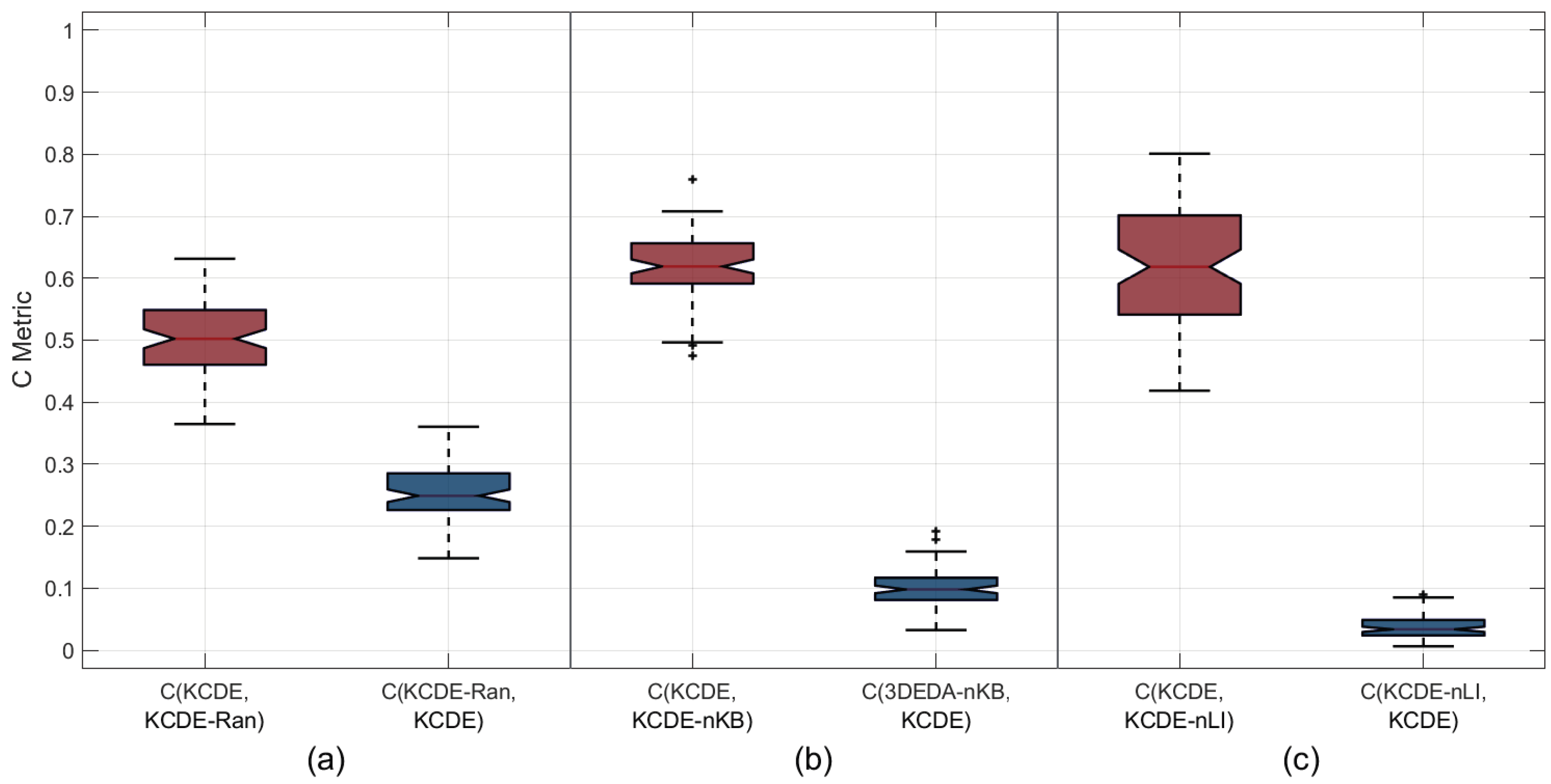
4.4. Effect of Hybrid Initialization

The proposed KCDE is compared to its variant KCDE-Ran, in which the initial population is generated randomly in order to investigate the effectiveness of hybrid initialization. For each instance, each algorithm runs 10 times independently. The average C(KCDE, KCDE-Ran) and C(KCDE-Ran, KCDE) values of the instances with the same scale are calculated and provided in Table 4. Furthermore, the p-value of the nonparametric test with a 95% confidence level is calculated and summarized for each scale (to analyze the significance of the difference between the two compared algorithms). The boxplots of all C M values are illustrated in Figure 5a.
It can be seen from Table 4 and Figure 5a that for each instance, C(KCDE, KCDE-Ran) is larger than C(KCDE-Ran, KCDE) while all p-values are smaller than 0.05. Therefore, it can be concluded that most of the non-dominated solutions obtained by KCDE are better than those provided by KCDE-Ran and the hybrid initialization considerably enhances the quality of the initial population (and, thus, the performance of KCDE).

4.5. Effect of Knowledge Base

In order to examine the effectiveness of the knowledge base, the comparisons between KCDE and its variant KCDE-nKB were carried out. In KCDE-nKB, each offspring is generated with the information carried out by the corresponding selected parents. Each algorithm runs 10 times independently, the average C M values of the instances with the same scale are calculated. Moreover, to analyze the significance of the difference between KCDE and KCDE-nKB, the sign test with a 95% confidence level was carried out, and the p-value of each scale is calculated and summarized in Table 5. The boxplots of all C M values are provided in Figure 5b.
From Table 5 and Figure 5b, it is obvious that C(KCDE,KCDE-nKB) is larger than C(KCDE-nKB,KCDE) for each instance and all p-values are lower than 0.05, which demonstrates that most solutions in the Pareto set approximation obtained by KCDE are better than those yielded by KCDE-nKB. Thus, it can be concluded that the utilization of the knowledge base can efficiently support KCDE by providing information carried out by elite individuals.

4.6. Effect of Local Intensification

The effectiveness of local intensification is investigated by comparing the proposed KCDE and KCDE-nLI, in which the local intensification part is absent. The average C(KCDE,KCDE-nLI) and C(KCDE-nLI, KCDE) values of the instances with the same scales were calculated and summarized in Table 6. Furthermore, to analyze the significance of the difference between the two algorithms, the sign test with the 95% confidence level was carried out and the p-values were calculated. The boxplots of all C M values are provided in Figure 5c.
As shown in Table 6 and Figure 5c, for each instance, C(KCDE,KCDE-nLI) is larger than C(KCDE-nLI, KCDE). Moreover, all of the p-values are lower than 0.05; it can be concluded that most elite solutions yielded by KCDE can dominate those obtained by KCDE-nLI. Thus, it can be concluded that the proposed local intensification operator has significant influence on enhancing the performance of KCDE.

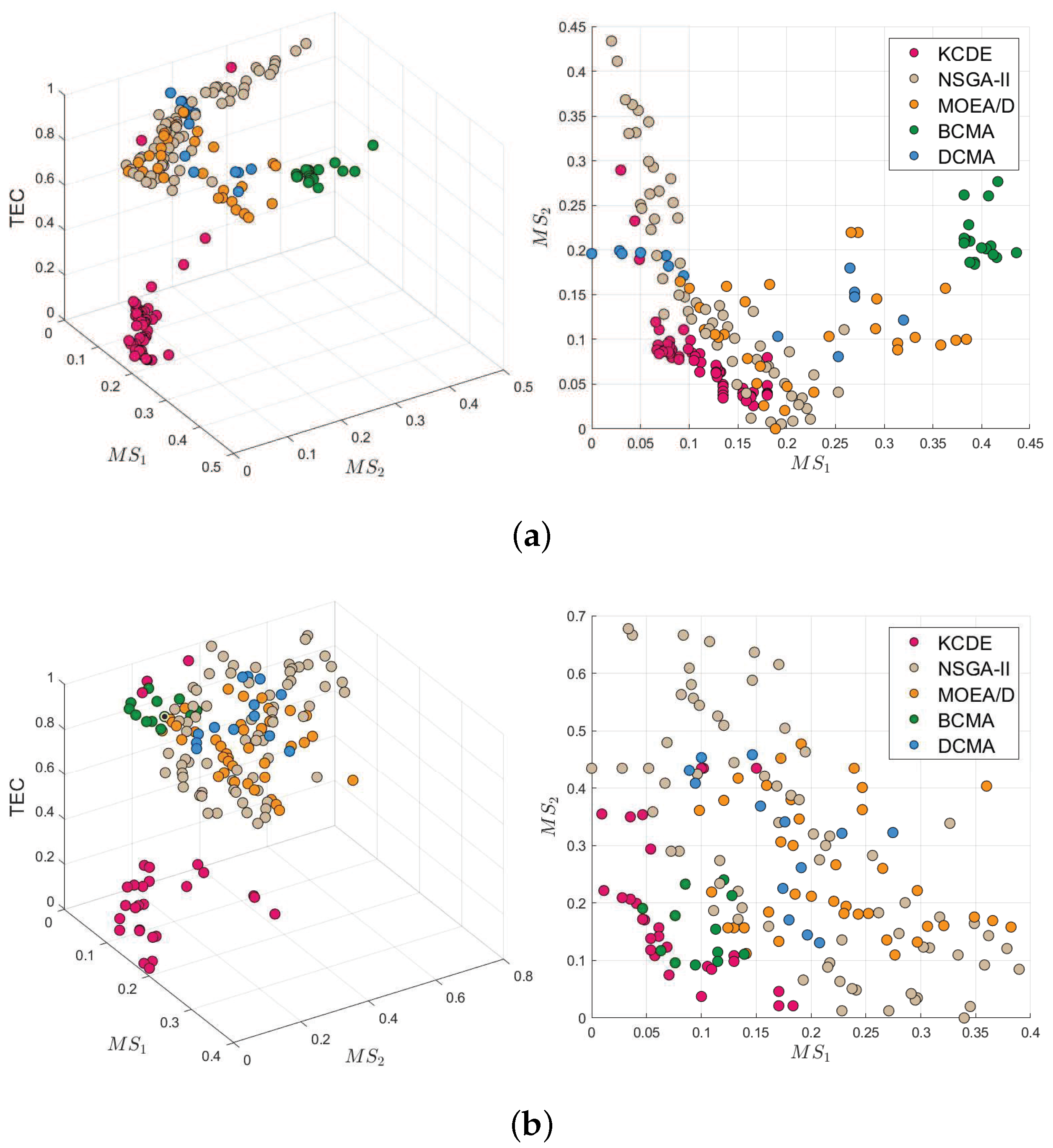
4.7. Comparisons to Other Algorithms

To our knowledge, there is currently no research on EDHFRP. Therefore, two state-of-the-art algorithms designed for problems similar to EDHFRP, i.e., DCMA [11] and BCMA [7], along with two classical multi-objective optimization algorithms, namely NSGA-II [49] and MOEA/D [50], were adapted for comparison. The parameters of DCMA and BCMA were set as suggestions in [7,11], respectively. The stopping criterion and running times are set as mentioned before.
The performances of all of the algorithms on instances of different scales are first evaluated by the C metric, which describes the dominant relationship between Pareto set approximations obtained by different algorithms. The average C M between KCDE and the other 4 algorithms in 10 instances of each scale are indicated in Table 7, while Figure 6 represents the boxplots of all C M . Moreover, the nonparametric test with a confidence level of 95% is carried out to show if there are significant differences between different algorithms; the p values are also recorded in Table 7. It is noticeable that C(KCDE, NSGA-II), C(KCDE, MOEA/D), C(KCDE, BCMA), and C(KCDE, DCMA) are much larger than C(NSGA-II, KCDE), C(MOEA/D, KCDE), C(BCMA, KCDE), and C(DCMA, KCDE) in all instances of different scales, especially large-scale instances. Moreover, the p values are all lower than 0.05, which indicates that most of the solutions obtained by KCDE can dominate those of the other algorithms. Therefore, it can be demonstrated that KCDE performs significantly better than NSGA-II, MOEA/D, BCMA, and DCMA.
The average HV and GD values of all algorithms are provided in Table 8. Figure 7 and Figure 8 illustrate the boxplots of two evaluation indicators on instances of different scales and the distribution of Pareto set approximations respectively. For each instance, the objective values are normalized with the largest value and the lowest value obtained by all the algorithms as higher bounds and lower bounds, respectively.
From Table 8 and Figure 7, one can see that the KCDE results in higher HV and lower GD in all instances. Thus, KCDE performs better than NSGA-II, MOEA/D, BCMA, and DCMA in solving EDHFRP since higher HV values indicate better convergence and diversity of the Pareto set approximations while lower GD values represent greater convergence properties. The Pareto set approximations of five algorithms in instances f3n30+30s5 and f3n80+20s5 are displayed in Figure 8, from which one can observe that the non-dominated solutions achieved by KCDE distribute more evenly than those obtained by the other four algorithms. As a result, it can be concluded that KCDE is more able to provide better solutions with shorter makespans and lower total energy consumption for EDHFRP.

5. Conclusions

This paper focuses on solving the energy-efficient distributed hybrid flow-shop rescheduling problem, minimizing the makespans of original and newly arrived orders as well as the total energy consumption, simultaneously. To this end, a knowledge-based cooperative differential evolution algorithm was designed. A group of broad instances with stochastic arrival times for the new order were generated. The effects of major parameters on the proposed algorithm were investigated and the importance of each problem-specific strategy was verified through extensive tests and experiments. The comprehensive comparisons and analysis demonstrate that KCDE is able to perform in a superior way in each instance.
In the future, the proposed algorithm can be extended to solve distributed rescheduling problems with more complicated constraints, such as fuzzy processing time, sequence-dependent setup time, and limited buffers. Moreover, this work can be used to solve scheduling problems in other kinds of environments, including no-idle, no-wait, lot-streaming, and heterogeneous factories, by simply changing the model. Moreover, optimization objectives with more practical significance, including tardiness, time-of-use electricity costs, and transportation can be considered in the algorithm.

Author Contributions

Conceptualization, Y.D. and L.D.; methodology, Y.D. and L.D.; software, Y.D., L.D. and T.L.; validation, Y.D. and T.L.; formal analysis, Y.D. and L.D.; investigation, Y.D.; resources, Y.D.; data curation, Y.D. and T.L.; writing—original draft preparation, Y.D.; funding acquisition, L.D. All authors have read and agreed to the published version of the manuscript.

Funding

This work is supported by National Key R&D Program of China (Grant No.2022YFB3304002), National Natural Science Foundation of China (Grant No.62176075) and Natural Science Foundation of Shandong Province, China (Grant No.ZR2021MF063).

Institutional Review Board Statement

Not applicable.

Informed Consent Statement

Not applicable.

Data Availability Statement

The data are available upon request from the corresponding author.

Conflicts of Interest

The authors declare no conflict of interest.

References

  1. Gao, K.; Huang, Y.; Sadollah, A.; Wang, L. A review of energy-efficient scheduling in intelligent production systems. Complex Intell. Syst. 2020, 6, 237–249. [Google Scholar] [CrossRef]
  2. Wang, Y.; Guo, C.; Chen, X.; Jia, L.; Guo, X.; Chen, R.; Zhang, M.; Chen, Z.; Wang, H. Carbon peak and carbon neutrality in China: Goals, implementation path and prospects. China Geol. 2021, 4, 720–746. [Google Scholar] [CrossRef]
  3. Fu, Y.; Hou, Y.; Wang, Z.; Wu, X.; Gao, K.; Wang, L. Distributed scheduling problems in intelligent manufacturing systems. Tsinghua Sci. Technol. 2021, 26, 625–645. [Google Scholar] [CrossRef]
  4. Li, J.; Song, M.; Wang, L.; Duan, P.; Han, Y.; Sang, H.; Pan, Q. Hybrid artificial bee colony algorithm for a parallel batching distributed flow-shop problem with deteriorating jobs. IEEE Trans. Cybern. 2020, 50, 2425–2439. [Google Scholar] [CrossRef] [PubMed]
  5. Zhao, F.; Xu, Z.; Wang, L.; Zhu, N.; Xu, T.; Jonrinaldi. A population-based iterated greedy algorithm for distributed assembly no-wait flow-shop scheduling problem. IEEE Trans. Ind. Inform. 2022, 1–12, early access. [Google Scholar] [CrossRef]
  6. Zhao, F.; Ma, R.; Wang, L. A self-learning discrete Jaya algorithm for multiobjective energy-efficient distributed no-idle flow-shop scheduling problem in heterogeneous factory system. IEEE Trans. Cybern. 2022, 52, 12675–12686. [Google Scholar] [CrossRef] [PubMed]
  7. Wang, J.; Wang, L. A bi-population cooperative memetic algorithm for distributed hybrid flow-shop scheduling. IEEE Trans. Emerg. Top. Comput. Intell. 2021, 5, 947–961. [Google Scholar] [CrossRef]
  8. Pan, Z.; Lei, D.; Wang, L. A knowledge-based two-population optimization algorithm for distributed energy-efficient parallel machines scheduling. IEEE Trans. Cybern. 2022, 52, 5051–5063. [Google Scholar] [CrossRef]
  9. Pan, Q.; Gao, L.; Wang, L. An effective cooperative co-evolutionary algorithm for distributed flowshop group scheduling problems. IEEE Trans. Cybern. 2022, 52, 5999–6012. [Google Scholar] [CrossRef]
  10. Shao, W.; Shao, Z.; Pi, D. An ant colony optimization behavior-based MOEA/D for distributed heterogeneous hybrid flow shop scheduling problem under nonidentical time-of-use electricity tariffs. IEEE Trans. Cybern. 2022, 19, 3379–3394. [Google Scholar] [CrossRef]
  11. Zhang, G.; Liu, B.; Wang, L.; Yu, D.; Xing, K. Distributed co-evolutionary memetic algorithm for distributed hybrid differentiation flowshop scheduling problem. IEEE Trans. Evol. Comput. 2022, 26, 1043–1057. [Google Scholar] [CrossRef]
  12. Jiang, E.; Wang, L.; Wang, J. Decomposition-based multi-objective optimization for energy-aware distributed hybrid flow shop scheduling with multiprocessor tasks. Tsinghua Sci. Technol. 2021, 26, 646–663. [Google Scholar] [CrossRef]
  13. Li, J.; Chen, X.; Duan, P.; Mou, J. KMOEA: A knowledge-based multiobjective algorithm for distributed hybrid flow shop in a prefabricated system. IEEE Trans. Ind. Informatics 2022, 18, 5318–5329. [Google Scholar] [CrossRef]
  14. Framinan, J.M.; Viagas, V.F.; Gonzalez, P.P. Using real-time information to reschedule jobs in a flowshop with variable processing times. Comput. Ind. Eng. 2019, 129, 113–125. [Google Scholar] [CrossRef]
  15. Gao, K.; Yang, F.; Zhou, M.; Pan, Q.; Suganthan, P.N. Flexible Job-shop rescheduling for new job insertion by using discrete Jaya algorithm. IEEE Trans. Cybern. 2019, 49, 1944–1955. [Google Scholar] [CrossRef]
  16. Gao, K.; Yang, F.; Li, J.; Sang, H.; Luo, J. Improved Jaya algorithm for flexible job shop rescheduling problem. IEEE Access 2020, 8, 86915–86922. [Google Scholar] [CrossRef]
  17. Nouiri, M.; Bekrar, A.; Trentesaux, D. Towards energy efficient scheduling and rescheduling for dynamic flexible job shop problem. IFAC-PapersOnLine 2018, 51, 1275–1280. [Google Scholar] [CrossRef]
  18. An, Y.; Chen, X.; Gao, K.; Zhang, L.; Li, Y.; Zhao, Z. A hybrid multi-objective evolutionary algorithm for solving an adaptive flexible job-shop rescheduling problem with real-time order acceptance and condition-based preventive maintenance. Swarm Evol. Comput. 2023, 77, 101243. [Google Scholar] [CrossRef]
  19. An, Y.; Chen, X.; Gao, K.; Zhang, L.; Li, Y.; Zhao, Z. Integrated optimization of real-time order acceptance and flexible job-shop rescheduling with multi-level imperfect maintenance constraints. Expert Syst. Appl. 2023, 212, 178711. [Google Scholar] [CrossRef]
  20. Lv, Y.; Li, C.; Tang, Y.; Kou, Y. Toward energy-efficient rescheduling decision mechanisms for flexible job shop with dynamic events and alternative process plans. IEEE Trans. Autom. Sci. Eng. 2022, 19, 3259–3275. [Google Scholar] [CrossRef]
  21. Wang, Z.; Shen, L.; Li, X.; Gao, L. An improved multi-objective firefly algorithm for energy-efficient hybrid flowshop rescheduling problem. J. Clean. Prod. 2023, 385, 135738. [Google Scholar] [CrossRef]
  22. Li, J.; Pan, Q.; Mao, K. A hybrid fruit fly optimization algorithm for the realistic hybrid flowshop rescheduling problem in steelmaking systems. IEEE Trans. Autom. Sci. Eng. 2016, 13, 932–949. [Google Scholar] [CrossRef]
  23. Peng, K.; Pan, Q.; Gao, L.; Li, X.; Das, S.; Zhao, B. A multi-start variable neighbourhood descent algorithm for hybrid flowshop rescheduling. Swarm Evol. Comput. 2019, 45, 92–112. [Google Scholar] [CrossRef]
  24. Guo, Y.; Huang, M.; Wang, Q.; Leon, V.J. Single-machine rework rescheduling to minimize total waiting time with fixed sequence of jobs and release times. IEEE Access 2021, 9, 1205–1218. [Google Scholar] [CrossRef]
  25. Silva, N.C.O.; Scarpin, C.T.; Ruiz, A.; Pécora, J.E. Rescheduling production on identical parallel machines upon new jobs arrivals. IFAC-PapersOnLine 2019, 52, 2525–2530. [Google Scholar] [CrossRef]
  26. Storn, R.; Price, K. Differential evolution—A simple and efficient heuristic for global optimization over continuous spaces. J. Glob. Optim. 1997, 11, 341–359. [Google Scholar] [CrossRef]
  27. Opara, K.R.; Arabas, J. Differential evolution: A survey of theoretical analyses. Swarm Evol. Comput. 2019, 44, 546–558. [Google Scholar] [CrossRef]
  28. Zhang, W.; Wang, Y.; Yang, Y.; Gen, M. Hybrid multiobjective evolutionary algorithm based on differential evolution for flow shop scheduling problems. Comput. Ind. Eng. 2019, 130, 661–670. [Google Scholar] [CrossRef]
  29. Morais, M.F.; Ribeiro, M.; Silva, R.G.; Mariani, V.C.; Coelho, L. Discrete differential evolution metaheuristics for permutation flow shop scheduling problems. Comput. Ind. Eng. 2022, 166, 107956. [Google Scholar] [CrossRef]
  30. Santucci, V.; Baioletti, M.; Milani, A. Algebraic differential evolution algorithm for the permutation flowshop scheduling problem with total flowtime criterion. IEEE Trans. Evol. Comput. 2016, 20, 682–694. [Google Scholar] [CrossRef]
  31. Xue, L.; Wu, X. A multi-objective discrete differential evolution algorithm for energy-efficient two-stage flow shop scheduling under time-of-use electricity tariffs. Appl. Soft Comput. 2023, 133, 109946. [Google Scholar] [CrossRef]
  32. Li, H.; Wang, X.; Peng, J. A hybrid differential evolution algorithm for flexible job shop scheduling with outsourcing operations and job priority constraints. Expert Syst. Appl. 2022, 201, 117182. [Google Scholar] [CrossRef]
  33. Mahmoodjanloo, M.; Moghaddam, R.T.; Baboli, A.; Amiri, A.B. Flexible job shop scheduling problem with reconfigurable machine tools: An improved differential evolution algorithm. Appl. Soft Comput. 2020, 94, 106416. [Google Scholar] [CrossRef]
  34. Xu, Y.; Wang, L. Differential evolution algorithm for hybrid flow-shop scheduling problems. J. Syst. Eng. Electron. 2011, 22, 794–798. [Google Scholar] [CrossRef]
  35. Gao, D.; Wang, G.; Pedrycz, W. Solving fuzzy job-shop scheduling problem using DE algorithm improved by a selection mechanism. IEEE Trans. Fuzzy Syst. 2020, 28, 3265–3275. [Google Scholar] [CrossRef]
  36. Wang, G.; Gao, D.; Pedrycz, W. Solving multiobjective fuzzy job-shop scheduling problem by a hybrid adaptive differential evolution algorithm. IEEE Trans. Ind. Inform. 2022, 18, 8519–8528. [Google Scholar] [CrossRef]
  37. Wu, X.; Wang, L. Multiobjective differential evolution algorithm for solving robotic cell scheduling problem with batch-processing machines. IEEE Trans. Autom. Sci. Eng. 2021, 18, 757–775. [Google Scholar] [CrossRef]
  38. Zhou, S.; Xing, L.; Zheng, X.; Du, N.; Wang, L.; Zhang, Q. A self-adaptive differential evolution algorithm for scheduling a single batch-processing machine with arbitrary job sizes and release times. IEEE Trans. Cybern. 2021, 51, 1430–1442. [Google Scholar] [CrossRef]
  39. Nawaz, M.; Ensore, E.E.; Ham, I. A heuristic algorithm for the m-machine, n-job flow-shop sequencing problem. Omega 1983, 11, 91–95. [Google Scholar] [CrossRef]
  40. Viagas, V.F.; Ruiz, R.; Framinan, J.M. A new vision of approximate methods for the permutation flowshop to minimise makespan: State-of-the-art and computational evaluation. Eur. J. Oper. Res. 2017, 257, 707–721. [Google Scholar] [CrossRef]
  41. Wang, J.; Wang, L. A cooperative memetic algorithm with learning-based agent for energy-aware distributed hybrid flow-shop scheduling. IEEE Trans. Evol. Comput. 2022, 26, 1–14. [Google Scholar] [CrossRef]
  42. Zhao, F.; Di, S.; Wang, L. A hyperheuristic with Q-learning for the multiobjective energy-efficient distributed blocking flow shop scheduling problem. IEEE Trans. Cybern. 2022, 1–14, early access. [Google Scholar] [CrossRef]
  43. Bilal; Pant, M.; Zaheer, H.; Garcia-Hernandez, L.; Abraham, A. Differential evolution: A review of more than two decades of research. Eng. Appl. Artif. Intell. 2020, 90, 103479. [Google Scholar] [CrossRef]
  44. Das, S.; Mullick, S.S.; Suganthan, P.N. Recent advances in differential evolution—An updated survey. Swarm Evol. Comput. 2016, 27, 1–30. [Google Scholar] [CrossRef]
  45. Mahmud, S.; Abbasi, A.; Chakrabortty, R.K.; Ryan, M.J. Multi-operator communication based differential evolution with sequential Tabu Search approach for job shop scheduling problems. Appl. Soft Comput. 2021, 108, 107470. [Google Scholar] [CrossRef]
  46. Hou, Y.; Wu, Y.; Liu, Z.; Han, H.; Wang, P. Dynamic multi-objective differential evolution algorithm based on the information of evolution progress. Sci. China Technol. Sci. 2021, 64, 1676–1689. [Google Scholar] [CrossRef]
  47. Wu, X.; Liu, X.; Zhao, N. An improved differential evolution algorithm for solving a distributed assembly flexible job shop scheduling problem. Memetic Comput. 2019, 11, 335–355. [Google Scholar] [CrossRef]
  48. Zitzler, E.; Deb, K.; Thiele, L. Comparison of multiobjective evolutionary algorithms: Empirical results. Evol. Comput. 2000, 8, 173–195. [Google Scholar] [CrossRef] [PubMed]
  49. Deb, K.; Pratap, A.; Agarwal, S.; Meyarivan, T. A fast and elitist multiobjective genetic algorithm: NSGA-II. IEEE Trans. Evol. Comput. 2002, 6, 182–197. [Google Scholar] [CrossRef]
  50. Zhang, Q.; Li, H. MOEA/D: A multiobjective evolutionary algorithm based on decomposition. IEEE Trans. Evol. Comput. 2007, 11, 712–731. [Google Scholar] [CrossRef]
Figure 1. Gantt chart of an instance of EDHFRP; (a) Original schedule; (b) Reschedule.
Processes 11 00755 g001
Figure 2. A feasible solution of an instance of EDHFRP; (a) A feasible solution before new job arrival; (b) The solution after order O 2 ’s arrival.
Processes 11 00755 g002
Figure 3. Framework of KCDE for EDHFRP.
Processes 11 00755 g003
Figure 4. Main Effects Plot for F, C R and α .
Processes 11 00755 g004
Figure 5. Boxplots of C Metric of KCDE, KCDE-Ran, KCDE-nKB and KCDE-nLI; (a) Boxplots of KCDE and KCDE-Ran; (b) Boxplots of KCDE and KCDE-nKB; (c) Boxplots of KCDE and KCDE-nLI.
Processes 11 00755 g005
Figure 6. Boxplots of C Metric of KCDE, NSGA-II, MOEA/D, BCMA and DCMA.
Processes 11 00755 g006
Figure 7. Boxplots of HV and GD of KCDE, NSGA-II, MOEA/D, BCMA and DCMA; (a) Boxplots of HV; (b) Boxplots of GD.
Processes 11 00755 g007
Figure 8. Distribution of non-dominated solutions obtained by KCDE, NSGA-II, MOEA/D, BCMA and DCMA; (a) Non-dominated solutions on instance f3n30+30s5; (b) Non-dominated solutions on instance f3n80+20s5.
Processes 11 00755 g008
Table 1. Comparisons between CPLEX and KCDE.
InstanceOriginal OrderRescheduling Plan
CPLEXKCDECPLEXKCDE
f2n4+3s2117.7033.67117.7033.27119.10107.4068.34118.20107.4065.14
f2n4+3s2118.5033.02118.2032.66143.90143.0059.62143.80142.5058.70
f2n4+3s3123.0055.35123.0055.27166.00179.70103.55164.10178.2099.95
f2n4+3s3146.2061.90145.6061.43153.00195.1096.44153.00195.0094.55
f2n5+3s282.3044.0782.0043.23121.40119.0076.44121.30118.1074.04
f2n5+3s2150.2043.42150.2043.39149.60151.5079.13149.60151.5076.13
f2n5+3s3126.9058.47126.9058.48146.00102.90115.95145.70102.40113.76
f2n5+3s3200.6074.07200.6073.04228.90176.80121.70228.60176.00120.34
f3n5+3s296.3040.8895.9040.7199.10105.0099.8498.50103.0098.47
f3n5+3s2139.5040.53139.5040.51140.00142.3096.76138.80140.1096.32
The better value of each instance is marked in bold.
Table 2. Orthogonal Arrays and HV Values.
ExperimentFactor LevelHV
NumberF CR α
11110.77799
21220.76874
31330.78359
41440.78363
52120.77442
62210.77722
72340.78411
82430.78266
93130.77947
103240.78020
113310.78163
123420.78488
134140.77749
144230.77721
154320.77504
164410.78175
Table 3. Average HVs and the Rank of Each Parameter.
LevelF CR α
10.778490.777340.77965
20.779600.775840.77577
30.781540.781090.78073
40.777870.783230.78136
Delta0.003670.007380.00559
Rank312
The best value of each level is marked in bold.
Table 4. Average C Metric Values of KCDE and KCDE-Ran.
Dataset C 1 , 2 1 C 2 , 1 2pDataset C 1 , 2 C 2 , 1 pDataset C 1 , 2 C 2 , 1 p
f3n30+20s40.430.310.02f4n30+20s40.530.240.02f5n30+20s40.500.230.02
f3n30+20s50.470.340.02f4n30+20s50.440.320.02f5n30+20s50.450.290.02
f3n30+20s60.430.320.02f4n30+20s60.430.290.02f5n30+20s60.390.310.02
f3n30+30s40.470.300.02f4n30+30s40.500.300.02f5n30+30s40.450.280.02
f3n30+30s50.520.270.02f4n30+30s50.530.240.00f5n30+30s50.560.240.00
f3n30+30s60.530.280.02f4n30+30s60.460.360.02f5n30+30s60.530.250.02
f3n30+50s40.610.190.00f4n30+50s40.530.280.02f5n30+50s40.580.230.02
f3n30+50s50.540.260.02f4n30+50s50.530.270.02f5n30+50s50.540.230.02
f3n30+50s60.490.350.02f4n30+50s60.480.310.02f5n30+50s60.610.190.00
f3n50+20s40.420.280.02f4n50+20s40.470.260.02f5n50+20s40.440.240.00
f3n50+20s50.530.280.02f4n50+20s50.410.280.02f5n50+20s50.460.320.02
f3n50+20s60.480.290.02f4n50+20s60.500.240.00f5n50+20s60.460.320.02
f3n50+30s40.540.190.02f4n50+30s40.550.240.02f5n50+30s40.480.290.02
f3n50+30s50.570.270.02f4n50+30s50.460.330.02f5n50+30s50.540.260.02
f3n50+30s60.510.290.02f4n50+30s60.510.260.02f5n50+30s60.490.300.02
f3n50+50s40.600.220.02f4n50+50s40.580.230.00f5n50+50s40.570.220.00
f3n50+50s50.630.200.02f4n50+50s50.560.260.02f5n50+50s50.620.190.00
f3n50+50s60.590.240.02f4n50+50s60.570.230.00f5n50+50s60.590.230.00
f3n80+20s40.470.190.02f4n80+20s40.450.260.02f5n80+20s40.400.220.02
f3n80+20s50.500.280.02f4n80+20s50.430.220.02f5n80+20s50.520.220.00
f3n80+20s60.450.290.02f4n80+20s60.490.240.02f5n80+20s60.360.230.02
f3n80+30s40.480.180.02f4n80+30s40.470.220.02f5n80+30s40.480.150.00
f3n80+30s50.550.240.02f4n80+30s50.460.270.02f5n80+30s50.500.290.02
f3n80+30s60.470.240.02f4n80+30s60.560.200.00f5n80+30s60.440.280.02
f3n80+50s40.520.230.02f4n80+50s40.540.240.02f5n80+50s40.620.160.00
f3n80+50s50.570.190.02f4n80+50s50.500.260.02f5n80+50s50.600.230.02
f3n80+50s60.520.210.02f4n80+50s60.550.190.02f5n80+50s60.600.220.02
1C1,2 = C(KCDE,KCDE-Ran); 2 C2,1 = C(KCDE-Ran,KCDE).
Table 5. Average C Metric Values of KCDE and KCDE-nKB.
Dataset C 1 , 3 1 C 3 , 1 2pDataset C 1 , 3 C 3 , 1 pDataset C 1 , 3 C 3 , 1 p
f3n30+20s40.680.110.00f4n30+20s40.680.120.00f5n30+20s40.640.090.00
f3n30+20s50.640.150.00f4n30+20s50.530.180.02f5n30+20s50.700.070.00
f3n30+20s60.610.130.00f4n30+20s60.650.110.00f5n30+20s60.630.100.00
f3n30+30s40.670.100.00f4n30+30s40.620.120.02f5n30+30s40.700.060.00
f3n30+30s50.680.120.00f4n30+30s50.670.090.00f5n30+30s50.710.080.00
f3n30+30s60.650.090.00f4n30+30s60.700.120.00f5n30+30s60.690.120.00
f3n30+50s40.640.090.00f4n30+50s40.650.110.02f5n30+50s40.760.060.00
f3n30+50s50.610.190.02f4n30+50s50.680.100.00f5n30+50s50.670.090.00
f3n30+50s60.580.120.00f4n30+50s60.590.110.00f5n30+50s60.650.090.00
f3n50+20s40.550.110.00f4n50+20s40.600.100.00f5n50+20s40.590.090.00
f3n50+20s50.580.160.00f4n50+20s50.550.150.00f5n50+20s50.670.100.00
f3n50+20s60.610.090.00f4n50+20s60.540.120.00f5n50+20s60.670.100.00
f3n50+30s40.590.070.00f4n50+30s40.680.090.00f5n50+30s40.650.070.00
f3n50+30s50.660.090.00f4n50+30s50.590.100.00f5n50+30s50.660.110.00
f3n50+30s60.620.070.00f4n50+30s60.590.120.02f5n50+30s60.620.090.00
f3n50+50s40.650.070.00f4n50+50s40.610.100.00f5n50+50s40.610.100.00
f3n50+50s50.600.110.00f4n50+50s50.620.120.00f5n50+50s50.620.120.00
f3n50+50s60.660.090.00f4n50+50s60.590.120.00f5n50+50s60.560.130.00
f3n80+20s40.500.080.00f4n80+20s40.630.120.00f5n80+20s40.490.100.00
f3n80+20s50.590.080.00f4n80+20s50.600.110.00f5n80+20s50.570.140.02
f3n80+20s60.550.090.00f4n80+20s60.600.120.02f5n80+20s60.470.120.00
f3n80+30s40.580.060.00f4n80+30s40.650.070.00f5n80+30s40.520.110.00
f3n80+30s50.650.030.00f4n80+30s50.610.060.00f5n80+30s50.650.080.02
f3n80+30s60.590.050.00f4n80+30s60.610.080.00f5n80+30s60.580.100.00
f3n80+50s40.560.060.00f4n80+50s40.640.050.00f5n80+50s40.590.050.00
f3n80+50s50.580.070.00f4n80+50s50.670.040.00f5n80+50s50.640.080.00
f3n80+50s60.580.080.00f4n80+50s60.630.070.00f5n80+50s60.610.090.00
1C1,3 = C(KCDE,KCDE-nKB); 2 C3,1 = C(KCDE-nKB,KCDE).
Table 6. Average C Metric Values of KCDE and KCDE-nLI.
Dataset C 1 , 4 1 C 4 , 1 2pDataset C 1 , 4 C 4 , 1 pDataset C 1 , 4 C 4 , 1 p
f3n30+20s40.670.030.00f4n30+20s40.730.020.00f5n30+20s40.660.030.00
f3n30+20s50.550.030.00f4n30+20s50.640.030.02f5n30+20s50.670.030.00
f3n30+20s60.550.050.00f4n30+20s60.720.020.00f5n30+20s60.630.030.00
f3n30+30s40.590.020.00f4n30+30s40.750.020.00f5n30+30s40.650.030.00
f3n30+30s50.560.030.00f4n30+30s50.720.020.00f5n30+30s50.710.010.00
f3n30+30s60.650.030.00f4n30+30s60.780.010.00f5n30+30s60.690.020.00
f3n30+50s40.650.030.00f4n30+50s40.710.020.00f5n30+50s40.800.010.00
f3n30+50s50.530.020.00f4n30+50s50.790.010.00f5n30+50s50.720.010.00
f3n30+50s60.620.030.00f4n30+50s60.740.010.00f5n30+50s60.790.010.00
f3n50+20s40.560.070.00f4n50+20s40.690.040.00f5n50+20s40.630.030.00
f3n50+20s50.510.070.02f4n50+20s50.700.040.00f5n50+20s50.610.050.00
f3n50+20s60.480.060.00f4n50+20s60.580.050.00f5n50+20s60.610.050.00
f3n50+30s40.630.050.00f4n50+30s40.750.030.00f5n50+30s40.710.020.00
f3n50+30s50.520.060.00f4n50+30s50.680.030.00f5n50+30s50.620.020.00
f3n50+30s60.520.050.00f4n50+30s60.580.050.00f5n50+30s60.660.030.00
f3n50+50s40.620.040.00f4n50+50s40.780.030.00f5n50+50s40.740.020.00
f3n50+50s50.510.040.00f4n50+50s50.720.020.00f5n50+50s50.670.010.00
f3n50+50s60.470.040.00f4n50+50s60.530.040.00f5n50+50s60.660.020.00
f3n80+20s40.550.090.02f4n80+20s40.590.050.00f5n80+20s40.600.040.00
f3n80+20s50.460.090.02f4n80+20s50.560.050.02f5n80+20s50.570.040.00
f3n80+20s60.480.080.00f4n80+20s60.500.070.00f5n80+20s60.580.040.00
f3n80+30s40.520.070.00f4n80+30s40.660.040.00f5n80+30s40.590.050.00
f3n80+30s50.440.080.02f4n80+30s50.570.060.02f5n80+30s50.520.040.02
f3n80+30s60.480.080.02f4n80+30s60.420.060.02f5n80+30s60.710.040.02
f3n80+50s40.490.050.00f4n80+50s40.710.040.00f5n80+50s40.710.030.00
f3n80+50s50.430.060.02f4n80+50s50.590.030.00f5n80+50s50.600.020.00
f3n80+50s60.460.050.00f4n80+50s60.440.050.00f5n80+50s60.700.020.00
1C1,4 = C(KCDE,KCDE-nLI); 2 C4,1 = C(KCDE-nLI,KCDE).
Table 7. Average C Metric Values of KCDE and NSGA-II, MOEA/D, BCMA, DCMA.
Dataset C 1 , 5 1 C 5 , 1 2p C 1 , 6 3 C 6 , 1 4p C 1 , 7 5 C 7 , 1 6p C 1 , 8 7 C 8 , 1 8p
f3n30+200.7350.0180.000.7960.0140.000.5170.0130.000.7050.0000.00
f3n30+300.7630.0130.000.7920.0110.000.5000.0100.000.5950.0000.00
f3n30+500.7310.0120.000.7520.0120.000.4890.0080.000.3810.0000.00
f3n50+200.6760.0340.000.7680.0220.000.5210.0220.000.8980.0000.00
f3n50+300.7490.0210.000.7920.0190.000.5610.0180.000.8200.0000.00
f3n50+500.7510.0140.000.8140.0140.000.5950.0090.000.7050.0000.00
f3n80+200.6740.0350.010.7100.0320.000.4460.0360.010.9520.0000.00
f3n80+300.6750.0310.000.7310.0270.000.4580.0260.000.9330.0000.00
f3n80+500.7400.0240.010.7680.0200.000.5470.0180.010.9030.0000.00
f4n30+200.7840.0110.000.8420.0110.000.4990.0080.000.7130.0000.00
f4n30+300.8270.0080.000.8510.0050.000.5320.0060.000.6340.0000.00
f4n30+500.8480.0040.000.8690.0030.000.4680.0040.000.5490.0000.00
f4n50+200.7700.0200.000.8210.0130.000.5670.0130.000.8600.0000.00
f4n50+300.8170.0110.000.8600.0120.000.5690.0110.000.7730.0000.00
f4n50+500.8470.0080.000.8900.0090.000.5780.0090.000.6530.0000.00
f4n80+200.7350.0260.000.7820.0150.000.5080.0180.010.9350.0000.00
f4n80+300.7720.0200.000.8130.0190.000.5630.0120.000.8950.0000.00
f4n80+500.8610.0100.000.8830.0100.000.5940.0090.000.8520.0000.00
f5n30+200.7690.0130.000.8020.0100.000.5190.0060.000.6450.0030.00
f5n30+300.8380.0060.000.8640.0040.000.5740.0040.000.4800.0010.00
f5n30+500.8310.0050.000.8630.0030.000.5230.0030.000.6560.0010.00
f5n50+200.7540.0110.000.8580.0060.000.5710.0070.000.8550.0000.00
f5n50+300.8180.0100.000.9100.0080.000.6430.0060.000.7640.0010.00
f5n50+500.8220.0070.000.9140.0040.000.6530.0050.000.8280.0000.00
f5n80+200.7030.0270.010.8240.0180.000.5210.0200.010.9460.0020.00
f5n80+300.7630.0170.010.8690.0100.000.5590.0110.000.9170.0010.00
f5n80+500.8230.0110.000.9130.0060.000.5620.0130.000.7980.0000.00
1C1,5 = C(KCDE,NSGA-II); 2 C5,1 = C(NSGA-II,KCDE); 3 C1,6 = C(KCDE,MOEA/D) ; 4 C6,1 = C(MOEA/D,KCDE); 5 C1,7 = C(KCDE,BCMA); 6 C7,1 = C(MOEA/D,BCMA); 7 C1,8 = C(KCDE,DCMA); 8 C8,1 = C(MOEA/D,DCMA).
Table 8. HVs and GDs of KCDE and NSGA-II, MOEA/D, BCMA, DCMA.
DatasetHVGD
KCDENSGAMOEA/DBCMADCMAKCDENSGAMOEA/DBCMADCMA
f3n30+200.850.100.100.080.040.131.061.021.001.40
f3n30+300.860.110.110.090.050.101.020.960.991.35
f3n30+500.860.120.110.100.060.090.950.911.001.26
f3n50+200.860.080.070.070.030.151.111.041.031.50
f3n50+300.880.090.090.070.030.111.060.991.031.45
f3n50+500.880.100.100.080.050.070.980.921.011.39
f3n80+200.870.060.060.050.020.181.161.081.071.56
f3n80+300.870.060.070.060.020.151.141.031.051.54
f3n80+500.890.080.080.070.030.091.020.981.031.51
f4n30+200.870.100.100.070.040.101.030.991.071.27
f4n30+300.900.110.110.080.050.070.980.951.041.22
f4n30+500.910.130.120.100.060.060.950.901.011.16
f4n50+200.880.070.070.050.020.121.091.021.131.46
f4n50+300.900.090.080.060.030.091.060.971.121.37
f4n50+500.900.100.100.080.050.060.990.921.091.27
f4n80+200.870.060.060.050.020.161.141.071.141.51
f4n80+300.890.060.060.050.020.121.091.021.141.47
f4n80+500.910.080.080.060.030.081.030.971.141.41
f5n30+200.840.090.090.060.050.171.091.051.071.36
f5n30+300.900.110.110.080.050.081.030.971.051.32
f5n30+500.910.130.120.090.040.070.970.921.041.40
f5n50+200.870.070.070.050.030.151.121.081.151.47
f5n50+300.910.080.080.060.040.081.061.011.131.42
f5n50+500.910.100.090.070.030.051.000.961.111.49
f5n80+200.850.050.050.040.020.201.201.141.171.54
f5n80+300.890.060.060.040.030.111.121.081.151.51
f5n80+500.910.070.070.050.040.071.051.001.121.36
Disclaimer/Publisher’s Note: The statements, opinions and data contained in all publications are solely those of the individual author(s) and contributor(s) and not of MDPI and/or the editor(s). MDPI and/or the editor(s) disclaim responsibility for any injury to people or property resulting from any ideas, methods, instructions or products referred to in the content.

