Article

Terminal Integral Synergetic Control for Wind Turbine at Region II Using a Two-Mass Model

by
Saravanakumar Rajendran
1,*,
Debashisha Jena
2,
Matias Diaz
1,* and
José Rodríguez
3
1
Department of Electrical Engineering, University of Santiago of Chile, Santiago 9170125, Chile
2
Department of Electrical and Electronics Engineering, National Institute of Technology Karnataka, Mangalore 575025, India
3
Engineering Faculty, Universidad San Sebastian, Santiago 4080871, Chile
*
Authors to whom correspondence should be addressed.
Processes 2023, 11(2), 616; https://doi.org/10.3390/pr11020616
Submission received: 21 January 2023 / Revised: 10 February 2023 / Accepted: 11 February 2023 / Published: 17 February 2023
(This article belongs to the Special Issue Advances in Wind Turbine Energy Conversion Systems)

Abstract

:
Mechanical loads considerably impact wind turbine lifetime, and a reduction in this load is crucial while designing a controller for maximum power extraction at below-rated speed (region II). A trade-off between maximum energy extraction and minimum load on the drive train shaft is a big challenge. Some conventional controllers extract the maximum power with a cost of high fluctuations in the generator torque and transient load. Therefore, to overcome the above issues, this work proposes four different integral synergetic control schemes for a wind turbine at region II using a two-mass model with a wind speed estimator. In addition, the proposed controllers have been developed to enhance the maximum power extraction from the wind whilst reducing the control input and drive train oscillations. Moreover, a terminal manifold has been considered to improve the finite time convergence rate. The effectiveness of the proposed controllers is validated through a 600 kW Fatigue, Aerodynamics, Structures, and Turbulence simulator. Further, the proposed controllers were tested by different wind spectrums, such as Kaimal, Von Karman, Smooth-Terrain, and NWTCUP, with different turbulent intensities (10% and 20%). The overall performance of the proposed and conventional controller was examined with 24 different wind speed profiles. A detailed comparative analysis was carried out based on power extraction and reduction in mechanical loads.

1. Introduction

Over the years, worldwide annual energy demand has increased due to industrial development and living standards. However, this rapid expansion and reduction in fossil fuels directed more attention towards renewable energy resources [1,2]. As a result, wind energy is a prominent developing source among other renewable energy sources. In addition, the total capacity of wind energy reached 847 GW in 2021, with a 14% growth compared to 2020 [3].
Wind Turbines (WTs) are majorly classified into two categories, such as Fixed-Speed WTs (FSWTs) and Variable-Speed WTs (VSWTs). However, VSWTs have many advantages over FSWTs. For instance, the VSWTs produce more annual energy yield than FSWTs [4]. In VSWT, Maximum Power Extraction (MPE) and transient load reduction are two significant factors. The operating regions of the VSWT are illustrated in Figure 1. In Region I (below cut-in wind speed), the available power in this region is lower than the WT losses. For this reason, the turbines are at a standstill condition. At below-rated wind speeds (Region II), WT extracts maximum power from the wind while reducing mechanical loads. In this region, the generator torque acts as a control input to the WT with an optimal pitch angle. In Region III (above-rated wind speed), the turbine limits the power capture at a rated value to protect against damage to the turbine. In this region, the pitch angle acts as a control input to the WT. Finally, Region IV refers to the above cutoff wind speed, and the turbines are at a standstill to avoid damaging turbine components.
This work focused on Region II, where torque control is essential to acquire the MPE whilst the oscillation on the transient load must be minimized. Therefore, achieving the MPE in the presence of uncertainties, unknown disturbances, and varying wind speeds is challenging for the torque controller. A detailed analysis of WT generators and power converters is presented in the Refs. [5,6]. An extensive investigation was conducted in the Ref. [7] for fault diagnosis, prognosis and resilient control methods for WECS. Classical controllers such as PI and PID are extensively utilized for MPE [8,9]. In the Ref. [10], the combination of PI control with the gain schedule method was adapted for better power capture. However, these classical control methods would not be able to consider the nonlinearities and do not take into account the dynamics of the wind and WT.
Nonlinear controllers play an influential role in MPE due to their variable structure and finite time reachability. Additionally, these control techniques have the following merits: robustness against parameter uncertainty, external disturbances, and unmodeled dynamics. Beltran et al. proposed sliding mode control (SMC) to ensure the stability of the WT concerning minimal and nonminimal phase regions with ideal feedback [11]. The performance of the controller is validated by a 1.5 MW National Renewable Energy Laboratory (NREL) wind turbine simulator. However, the rotor speed is not limited to the nominal value, which leads to high mechanical stress on the drive train. In the Ref. [12], four different SMCs were compared and concluded and the super-twisting algorithm presented the most promising performance in Region II than others. A super-twisting with variable gain has been designed for MPE and compared with the existing super-twisting control [13]. Additionally, a Lyapunov candidate function is utilized to confirm the stability of the algorithm. Nonlinear static and dynamic feedback linearization controllers with a Newton Raphson (NR)-based wind speed estimator for a single mass model and two mass-model of the VSWT were addressed in the Refs. [14,15] respectively. However, the efficacy of the controllers relies on the error dynamics, which may introduce high oscillations in the control input during highly turbulent wind speeds. In the Ref. [16], two sliding mode control (SMC) approaches were proposed for MPE. Moreover, the first strategy utilizes a wind speed estimator, and the second uses MPPT to achieve better tracking performance. In the Ref. [17], the authors discussed SMC and integral sliding mode control (ISMC) with a wind speed estimator for MPE in Region II. In addition, a detailed comparative analysis was presented and concluded that ISMC performs better than others. In the Ref. [18], a nonlinear controller with a variable parameter was implemented for MPE, where the proposed controller minimized the oscillation in the drive train by adjusting the control parameter. Authors in the Ref. [19] designed a multivariable gain scheduling controller in a transient zone and a monovariable controller was designed for regions II and III. In addition, a gain scheduling block was also utilized in the multivariable controller to smooth the transition between the regions. A current decoupling control was proposed in the Ref. [20] for the DFIG offshore floating WT system to achieve the MPE. In addition, the ISMC was employed to compensate for output error in the open-loop controller, and the parameters of this controller were optimized by Gray Wolf Optimization (GWO).
Three different synergetic control schemes for a two-mass model of VSWT with a wind estimator were presented in the Ref. [21]. Simulation results demonstrate that an integral controller based on the synergetic terminal improves transient load reduction over conventional controllers. Authors in the Ref. [22] proposed fast terminal synergetic control (FTSC) to enhance speed tracking and improve the MPE. The macro-variable in the FTSC enriches the convergence speed and reduces the chattering action of the control input. In the Ref. [23], two sliding surfaces, such as a proportional integral derivative (PID) sliding surface and a combination of a nonlinear terminal sliding surface with a PID sliding surface, were proposed to improve the performance of MPE and reduce mechanical stresses in region II. In addition, these strategies address the effects of parametric uncertainties, unmodeled dynamics, and external disturbances. In the Ref. [24], extreme machine learning was proposed to forecast wind speed, and state feedback control was employed to track the MPE. In the Ref. [25], the authors presented two nonlinear control approaches using an optimal fractional high-order fast terminal sliding mode (FHOFTSM) proposed to ensure the MPE and minimize the mechanical loads. The design process of FHOFTSM has two stages. In the first stage, an optimal controller is designed to minimize the nominal error based on the quadratic performance index. In the second stage, the switching controller is designed based on a fractional high-order and fractional nonsingular fast terminal sliding manifold. In the Ref. [26], a complementary SMC was proposed to improve the MPE at region II for VSWT. In the Ref. [27], a nonlinear terminal integral SMC was proposed for MPE in VSWT and implemented in a FAST simulator with nine degrees of freedom (DOFs). A super-twisting SMC (STSMC) with anti-disturbance capabilities was proposed in the Ref. [28] for doubly-fed induction generator-based WECS. In addition, an artificial neural network was utilized to enhance the performance of the STSMC. The authors in the Ref. [29] proposed the ISMC to improve MPE and reduce transient loads for large-scale WTs. Additionally, the proposed controller enhanced the chattering-free electromagnetic torque. In the Ref. [30], reference model adaptive control was proposed to achieve the MPE in WECS under realistic wind speed profiles. In addition, a recurrent neural network (RNN) was used to improve the measurement error. However, the above methods are complex, and the influence of the control input on the low-speed shaft torque measures the transient load on the drive train. Therefore, this work aims to design the controllers to mitigate the transient load and improve the MPE.
The main aim of the work was to extract the MPE at region II with minimum oscillation on the control input and low-speed shaft torque. Some conventional controllers are designed to improve the MPE with the cost of high control input. However, those control strategies introduce more stress on the drive train, which significantly affects the lifetime of the wind turbine. In WTs, a reasonable compromise should be made between energy extraction and dynamics loads on the drive train, which have become critical issues. Therefore, to address the issues, four different synergetic control schemes for VSWT at region II are proposed: integral synergetic control (ISC), terminal integral synergetic control (TISC), modified integral synergetic control (MISC), and terminal modified integral synergetic control (TMISC). In addition, the proposed controllers were designed based on the synergetic control theory, which considers the nonlinear dynamics of the WT using a two-mass model with a wind speed estimator.
The following are the significant contributions of this article.
  • The integral-based macro-variable is employed for designing the synergetic control schemes to enhance MPE from wind at region II whilst reducing control input and drive train oscillations.
  • A terminal synergetic manifold has been considered to improve the finite-time convergence rate. By utilizing these control strategies, the MPE can be improved with a minimum control input. Additionally, this terminal-based integral manifold has achieved better performance than other controllers.
  • A 600 kW FAST simulator is used to test the effectiveness of the proposed controllers. Moreover, various wind spectral models, such as Kaimal, Von Karman, Smooth-Terrain, and NWTCUP, with different turbulent intensities (10% and 20%) and mean wind speeds (7m/s, 8m/s and 8.5m/s), are examined for each controller.
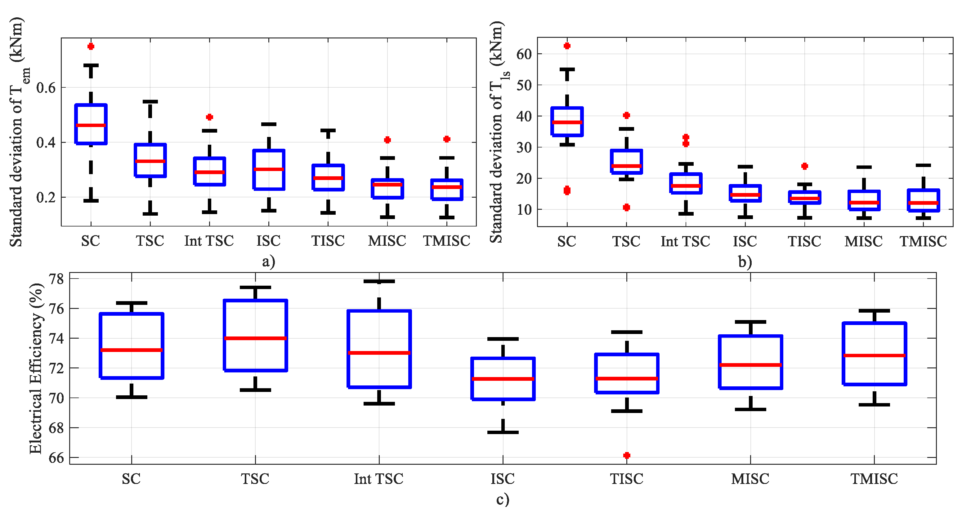
  • Finally, the overall performance of the proposed controllers was evaluated based on the 24 different wind speed profiles, and an extensive comparative analysis has been presented.

2. Wind Turbine Modeling

The dynamic modelling of the VSWT is described in this section. In addition, the model comprises aerodynamic & turbine characteristics and dynamics of a generator.

Description of the Model

The dynamic loads and interaction of the multiple components of WT require aeroelastic simulators. However, the mixture of aerodynamic loading and dynamics of various features demands a complex simulator. Therefore, many researchers have focused on structural loads and the aeroelasticity of the WT. This work mainly focuses on controller design for VSWT, so those complex simulators are unnecessary. A simplified mathematical model of WT exists in the literature, and those models are sufficient for controller design. A set of nonlinear differential equations describes the mathematical model of the WT with a limited DOF. The proposed controllers were designed based on the mathematical model of the WT for MPE.
The VSWT comprises the following major components, such as the aeroturbine, generator, and gearbox. Equation (1) describes the aerodynamic power ( P a ) which is captured by the rotor.
P a = P ω C p λ , β
where P ω = 1 2 ρ A υ 3 , where ρ is the density of the air ( k g m 3 ), A is the rotor area in ( m 2 ) and υ is the wind speed ( m s ).
The WT power coefficient ( C p ) relies on the tip speed ratio ( λ ) and blade pitch angle ( β ). The tip speed ratio is defined as
λ = ω r R υ
From Equation (2), it is clear that any change in wind speed or rotor speed produces a variation in the tip speed ratio, which causes variations in the power coefficient. The relationship between aerodynamic torque ( T a ) and aerodynamic power is given by (3).
P a = T a ω r
where
T a = 0.5 ρ π R 3 C q λ , β υ 2
C q λ , β = C p λ , β λ
Figure 2 depicts the power coefficient of the WT considered for this work. The surfaces of this figure were obtained using the blade element moment theory, which was implemented in the WT performance code and developed by NREL [31,32]. Finally, the look-up tables were utilized to execute these surfaces in the mathematical model of the WT.
The aerodynamic torque drives the inertia of the rotor ( J r (kg m2)) at a speed of ω r . Equation (6) describes the dynamics of the rotor.
J r ω r ˙ = T a T l s K r ω r
The braking torque in the rotor is influenced by the low-speed shaft torque ( T l s (Nm)), which is caused by the two angular velocities, such as the rotor speed and the low-speed shaft speed.
T l s = K l s θ r θ l s + B l s ω r ω l s
where K l s and B l s are the shaft damping (Nm/rad/s) and stiffness coefficient (Nm/rad), respectively. The high-speed shaft torque ( T h s ) drives the generator inertia ( J g (kg m2)) and is braked by the electromagnetic torque ( T e m ). Equation (8) describes the dynamics of the generator.
J g ω g ˙ = T h s K g ω g T e m
The gearbox transmits the torque and speed of the shaft in a gear ratio ( n g ). Equation (9) refers to the ideal gearbox.
n g = T l s T h s = ω g ω l s = θ g θ l s
The modelling of WT requires more additional mass and DOFs. In the Ref. [33], the WT model was developed with the assumption of flexibility on low- and high-speed shafts. In addition, some complex modelings are also considered for aeroturbines, where many rigid bodies are included [34,35]. In the Ref. [36], the authors discussed the six-mass, three-mass, and two-mass drive train models of the VSWT for transient stability analysis of the power system. This study concluded that the two-mass model is adequate for transient stability analysis with reasonable accuracy. Three different power electronics topologies with three different mass models were studied in the Ref. [37]. This study suggests that the three-mass model is useful for assessing the harmonics of the WT. In the Ref. [38], the structural dynamics of the rotor of FSWT and VSWT were analyzed. In this, both the shaft and the blade flexibilities increase the order of the model. Therefore, an adequate two-mass model has been considered with a reduction in the three-mass model. From the above discussion, it can be concluded that an effective two-mass model is sufficient to design the nonlinear controller for MPE.

3. Problem Formulation

The primary operating regions of the VSWT are given at wind speeds below and above. This work focuses mainly on Region II, and the main control objectives are as follows: (i). Extracts the maximum power. (ii). Reduction in transient loads.
Generally, the power capture curve has a unique maximum corresponding to wind power.
C p λ o p t , β o p t = C p o p t
λ o p t = ω o p t R υ
For MPE, the blade pitch angle is kept at optimal value β o p t . Further, to maintain λ at its optimal value, the rotor speed should track the reference speed. Equation (16) represents the reference rotor speed ( ω r e f ).
ω r e f = λ o p t υ R
From the above expression, it is clear that the shape of the reference rotor speed is similar to wind speed. Therefore, an optimal controller should track the reference rotor speed with minimum control stress and transient loads. Typically, the time constant of the electrical system is much smaller than the other components in the WT. Thus, there are two control cascade loops, namely the inner and outer loops. The inner loop takes into account an electrical generator and a power converter. In contrast, the outer loop considers an aeroturbine, which supplies a reference to the inner loop. Consider the assumption that the inner loops are well-controlled. However, this work mainly concentrates on designing a nonlinear controller for Region II, and the conventional pitch controller is adapted for Region III.

Effective Wind Speed Estimator

An anemometer is typically placed on the top of the nacelle to measure wind speed. This measured wind speed is defined as a point wind speed, which cannot be used to compute the effective wind speed. As the wind speed changes over the rotor-swept area, finding the effective wind speed is challenging. Thus, the effective wind speed is related to the aerodynamic torque and expressed in Equation (13).
T a = 1 2 ρ π R 3 C q ( λ ) v 2
where C q ( λ ) = C q λ , β o p t However, to solve Equation (13), the C q can be approximated using the polynomial λ .
C q λ = i = 1 n a i λ i
T ^ a 1 2 ρ π R 3 C q ω ^ r R v ^ v ^ 2 = 0
Therefore, to estimate the effective wind speed, the Newton–Raphson algorithm [14] is employed to solve the Equation (15). In addition, C q ( λ ) is approximated by the higher order polynomial of λ as given in Equation (14). Figure 3 presents the estimation of effective wind speed. For control purposes, the estimated reference speed is derived from the estimated effective wind speed, as given in Equation (16).
ω r e f ^ = λ o p t υ ^ R

4. Nonlinear Controllers

This section presents the design of the proposed controllers, such as ISC, TISC, MISC and TMISC, based on the two-mass model of the WT. In addition, the stability of the proposed controller was validated by the Lyapunov function.

4.1. Integral Synergetic Controller

The tracking error (e) is described as follows:
e = ω r ω r e f ^
Generally, the synergetic controller achieves the reference point with finite time convergence. Figure 4 presents the control structure of the proposed algorithms. The macro-variable of the controller depends on the error and maintains the state of the system in a specific manifold ψ 1 ( x , t ) = 0 . The integral synergetic controller is synthesized, and the macro-variable is defined as
ψ 1 = λ 1 e + λ 2 e
where ( λ 1 , λ 2 ) are positive constants. The main aim of the integral synergetic controller is to make the system on the manifold, provided the macro-variable is equivalent to zero. Equation (19) represents the dynamics of the macro-variable.
T ψ 1 ˙ + ψ 1 = 0
From the above equation, the control law relies not only on the macro-variable, but also on the control parameter (T). However, the design can decide the characteristics of the control law based on the selection of the macro-variable and control parameters. By taking the derivative of Equation (18),
ψ 1 ˙ = λ 1 e ˙ + λ 2 e
Combining Equations (17)–(19) guide to (21)
λ 1 e ˙ + λ 2 e = ψ 1 T
Substituting(6) into (21)
λ 1 T a J r T l s J r K r ω r J r ω r e f ^ ˙ + λ 2 e = ψ 1 T
T e m = T a η g K r ω r η g J g ω g ˙ K g ω g J r ω r e f ^ ˙ η g + J r λ 1 η g λ 2 e + ψ 1 T
Equation (23) defines the final control law for integral synergetic control. A low-pass filter was utilized to approximate the time derivative by s 1 + α s . However, the simulation time was too long for quite a small selection of α . Therefore, in this work, the α value chosen was 10.

4.2. Terminal Integral Synergetic Controller

The macro-variable defined in Equation (18) is considered, and the dynamics are defined as
T ψ 1 ˙ p q + ψ 1 = 0
where p and q are odd integers and must meet the following condition, 1 < p / q < 2 . Take the derivative of Equation (20) and substitute it into (24)
λ 1 T a J r T l s J r K r ω r J r ω r e f ^ ˙ + λ 2 e = ψ 1 T q p
T e m = T a η g K r ω r η g J g ω g ˙ K g ω g J r ω r e f ^ ˙ η g + J r λ 1 η g λ 2 e + ψ 1 T q p
Equation (26) defines the final control law for the integral synergetic control.

4.3. Modified Integral Synergetic Control

The macro-variable defined in Equation (18) is modified as follows:
ψ 2 = α 1 e a b + α 2 e + α 3 e
Furthermore, to validate the above expression, the following condition must be satisfied, that is, 1 < a / b < 2 if a and b are odd integers. Equation (28) defines the dynamics of the macrovariable based on the modified macrovariable defined in Equation (27).
τ ψ 2 ˙ + ψ 2 = 0
Taking the derivative of the Equation (27) leads to Equation (29)
ψ 2 ˙ = α 1 d d t e a b + α 2 e ˙ + α 3 e
Combining Equations (17), (27) and (28) leads to (30)
α 2 T a J r T l s J r K r ω r J r ω r e f ^ ˙ + α 1 d d t e a b + α 3 e = ψ 2 τ
Further, to find the control input to the WT, the above equation is modified
T e m = T a η g K r ω r η g J g ω g ˙ K g ω g J r ω r e f ^ ˙ η g + J r α 2 η g α 1 d d t e a b + α 3 e + ψ 2 τ
Equation (31) represents the modified integral synergetic control law for the WT to achieve MPE.

4.4. Terminal Modified Integral Synergetic Control

The macro-variable defined in Equation (27) is considered, and the dynamics of the macro-variable is defined as
τ ψ 2 ˙ p 1 q 1 + ψ 2 = 0
where p1 and q1 are odd integers and it should fulfil the following condition 1 < p 1 / q 1 < 2 .
Combining Equations (17), (27) and (32) leads to (33)
α 2 T a J r T l s J r K r ω r J r ω r e f ^ ˙ + α 1 d d t e a b + α 3 e = ψ 2 τ q 1 p 1
Further, the above equation is modified to derive the terminal modified integral synergetic control law as the control input to the WT.
T e m = T a η g K r ω r η g J g ω g ˙ K g ω g J r ω r e f ^ ˙ η g + J r α 2 η g α 1 d d t e a b + α 3 e + ψ 2 τ q 1 p 1
In all the proposed control schemes, the dynamics of the macro-variable are a function of error. The difference between the control structures depends on the definition of the macro-variable and the structure of the macro-variable. Equations (18) and (27) represent the definition of the macro-variables, and Equations (19) and (24) present the dynamics of the macro variables.

4.5. Stability Analysis

In this study, to validate the stability of the proposed controller, the following Lyapunov function ( V ϕ ) was considered.
V ϕ = 1 2 ψ 2 2 e
V ˙ = ψ 2 e ψ 2 ˙ e
V ˙ = ψ 2 ( e ) ψ ˙ 2 ( e ) = α 1 d d t e a b + α 2 e ˙ + α 3 e
The following equation was obtained by substituting the control law into (37).
V ˙ = ψ 2 e τ 1 α 1 d d t e a b + α 2 e ˙ + α 3 e
V ˙ = ψ 2 e τ 1 ψ 2 e
Equation (39) modified as
V ˙ = τ 1 ψ 2 2 e , τ > 0
The above equation shows the stability of the controller.

5. Validation Results

This section includes a detailed description of the Control Advanced Research Turbine (CART) WT model and an exhaustive analysis of the proposed and conventional controllers under various wind spectrum models and mean wind speeds.

5.1. Description about CART WT and FAST Model

The proposed controllers were validated through numerical simulations based on CART WT. The CART is the variable speed variable pitch WT with a squirrel cage induction generator. The generator is directly connected to the grid through a back-to-back Pulse Width Modulation (PWM) converter. It allows variable-speed operation by decoupling the rotor speed from the grid frequency. The generated power is injected directly into the grid by the supply-side converter. The front-end converter maintains the dc link voltage. A detailed description of the WT model is presented in the Ref. [39]. Figure 5 shows the wind speed that is generated by the SNWind. The Kaimal spectrum model with a turbulent intensity of 15% was considered to generate 600 s of wind speed. The sampling frequency of the wind speed depicted in Figure 5 is 400 Hz.
The NREL develops the Fatigue, Aerodynamics, Structures, and Turbulence (FAST) aeroelastic WT code and is employed to model two- or three-blade machines. Furthermore, WT designers used this code to forecast extreme and fatigue loads. The assumed model approach is used to represent the blade and tower components, while rigid bodies are used to describe the other components. Advanced certified codes are utilized to model the behavior of the WT. The blade element momentum (BEM) and a multicomponent wind speed profile are employed to find WT loads. Additionally, this code is certified by the Germanischer Lloyd (GL) WindEnergie GmbH [40]. Due to the above reasons, the proposed controllers have been verified by the FAST codes. This work considers the following DOFs: generator, rotor speed, and blade teeter. The DOFs for the generator and rotor speed are responsible for variations in the generator speed and drive train flexibility. In addition, the DOFs corresponding to the blade teeter include the asymmetric wind load across the rotor plane.

5.2. FAST Model Results

The main aim of the controllers is to optimize MPE while simultaneously reducing torque variations in the generator. Furthermore, torque variations could lead to increased mechanical stresses on the turbine. Consequently, optimal tracking of the rotor speed is impossible due to the rotor dynamics. Thus, intermediate tracking dynamics must be chosen to balance energy capture with reducing dynamic loads. Figure 6 and Figure 7 show the comparison of the rotor speed of all controllers. According to these figures, conventional and proposed controllers closely track the reference speed. However, the amount of control input required for an adequate tracking response must be considered to evaluate controllers. Furthermore, the effectiveness of the controllers depends not only on the MPE, but also on the standard deviation (STD) of the T e m and T l s . The following criteria have been considered to evaluate controllers: electrical and aerodynamic efficiency, STD, and maximum value of T e m and T l s . Equation (41) is used to find the electrical and aerodynamic efficiency.
η a e r o % = t i n i t f i n P a d t t i n i t f i n P a o p t d t ; η e l e % = t i n i t f i n P e d t t i n i t f i n P a o p t d t
where P a o p t = 0.5 ρ π R 2 C P o p t υ 3 is the optimal power.
Figure 8 and Figure 9 represent the electromagnetic torque of the conventional and proposed controllers. From these figures, one can see that conventional controllers introduce numerous oscillations in the control input. The designed torque with SC, TSC and Int TSC is longer than the proposed controllers. It shows that these controllers have substantial effects on the drive train. Therefore, the mechanical stress delivered by these controllers is greater than the proposed controllers. At the same time, the proposed controllers have a comparatively lesser variation in the control input. A detailed comparative study of conventional and proposed controllers is presented in Table 1. In this table, TSC and TISC have the highest and lowest electrical efficiency, respectively. Although TSC has the highest efficiency, the STDs of T e m and T l s are higher than the proposed controllers. In addition, examining Table 1, the STDs of T e m and T l s of SC and TIMSC have the highest and lowest out of the other controllers, respectively. It implies that the transient load on the drive train for TMISC has lower variations than others. A reasonable trade-off should be made between energy extraction and load reduction. Therefore, this analysis concludes that the proposed TIMSC is an acceptable control scheme compared to other controllers, although it has a little less efficiency than ISC.
The different wind speed spectrum suggested by the International Electrotechnical Commission (IEC) was utilised to find the efficacy of the proposed controllers. Generally, the nature of the wind speed is highly unpredictable; simultaneously, the mean wind speed also varies with time. Thus, to accommodate these conditions, different spectral models have been studied in this work. As a result, the TurbSim generates different spectral models, such as Kaimal, Von Karman, Smooth-Terrain, and NWTCUP, with a mean wind speed of 7, 8 and 8.5 m/s. In addition, these spectral models have turbulent intensities of 10% and 20%. Therefore, each controller is tested with four spectral models with two different intensities. The proposed and conventional controllers simulated eight different wind speed profiles for each mean wind speed.
Figure 10 shows a boxplot for the proposed and conventional controllers for various spectral models and mean wind speeds. The evaluation of the controllers was examined on the basis of the electrical efficiency and STD of T e m and T l s . Initially, the controllers were tested with a mean wind speed of 7m/s and different spectral models and intensities. According to Figure 10a,b, TIMSC and SC have the lowest and highest STD of T e m and T l s , respectively. It indicates that TISMC can minimize the oscillation in the control input and drive train in the presence of the different spectral models and intensities. By examining Figure 10c, the electrical efficiency of TSC is the highest among all the controllers, but this controller introduces more oscillations than TISMC. However, ISC, TISC and MISC have the lowest STD of T e m and T l s than conventional controllers. Subsequently, the electrical efficiency is lower than that of TMISC. This analysis concluded that, at an average wind speed of 7 m/s with various spectral models, TISMC performs better than other controllers.
The same analysis was performed with a mean wind speed of 8m/s. By examining Figure 10d–f, the effectiveness of the proposed and conventional controllers is similar to the mean wind speed of 7 m/s. From these figures, it can be seen that the STD of T e m and T l s of MISC and TMISC are close. It implies that the amount of control input required to track the reference speed of both controllers is almost similar. However, the electrical efficiency of TMISC is slightly higher than that of MISC. In addition, the controllers are also tested with a mean wind speed of 8.5 m/s. According to Figure 10g–i, the TMISC has the lowest STD of T e m , and the ISC has the lowest STD of T l s , which indicates that the TMISC minimizes the oscillation at the control input and the ISC minimizes the oscillation of the drive train. From this analysis, at a mean wind speed of 8.5 m/s with high turbulent intensity, the TMISC introduces a slightly higher oscillation on the drive train than ISC. At the same time, TMISC maintains electrical efficiency despite changes in mean wind speed. However, the ISC has a lower electrical efficiency than all controllers for different wind speed spectrums and mean wind speeds. This investigation implies that even though TMISC has a slightly higher STD of T l s than the ISC, the effectiveness of this control scheme is better than other controllers. The effectiveness of the controllers is analyzed during low and high turbulent intensities (10% and 20%) with different models of the wind spectrum. From the results, irrespective of the turbulent intensities, the proposed TMISC performed better in terms of electrical efficiency and lowest standard deviation of T e m and T l s than other controllers.
Figure 11 depicts a boxplot for the overall performance of the controllers. In the figure, 24 wind speed profiles are utilized to determine the overall effectiveness of the controllers. Figure 11a–c presents the overall STD of T e m , T l s and electrical efficiency. It demonstrates that despite different spectral models and mean wind speeds, the TMISC has the lowest STD of T e m and T l s among other controllers. The performance of MISC is almost similar to that of TMISC because the overall performance of these two is identical with respect to the control input and oscillation in the drive train. However, considering the electrical efficiency, the TMISC is higher than the MISC. Thus, a fair trade-off has to be made between electrical efficiency and drive train oscillations. Therefore, at high wind speeds (near rated wind speed), the controllers, such as MISC and TISMC, perform similarly, whereas at low wind speeds (near cut-in wind speed), TIMSC performs better than MISC.

6. Conclusions

This paper addressed issues such as MPE and the reduction in transient loads in VSWT operating in region II. Four different integral synergetic control schemes based on the two-mass model of the WT with a wind speed estimator have been proposed. In addition, a terminal manifold improves finite-time convergence with a minimum control input. Furthermore, a 600 kW FAST wind simulator has been utilized to demonstrate the effectiveness of the proposed controllers and compare them with some conventional controllers. By comparing the performance of the controllers, MISC and TMISC performed much better than other proposed and conventional controllers. At the same time, the electrical efficiency of conventional controllers, such as SC, TSC, and Int TSC was slightly higher than that of the proposed controllers. However, the standard deviation of these controllers is very high compared to the proposed controllers. It implies that these controllers require a high control input for MPE whilst introducing more oscillations in the drive train. Furthermore, four different wind spectral models have been investigated with different turbulent intensities and mean wind speeds. From this analysis, the proposed TMISC achieves the control objectives at 7 m/s, and for 8 and 8.5 m/s. In the future, the proposed control schemes can adapt to the small WTs, and the extension of TMISC with an evolutionary algorithm will further improve the efficacy of the controller.

Author Contributions

Conceptualization S.R. and D.J.; methodology, S.R., D.J. and M.D.; validation, S.R. and D.J.; investigation, S.R., D.J. and M.D.; writing—original draft preparation, S.R. and D.J.; writing—review and editing, D.J., M.D. and J.R.; supervision, D.J., M.D. and J.R. All authors have read and agreed to the published version of the manuscript.

Funding

This research was funded by Agencia Nacional de Investigación y Desarrollo (ANID) of Chile, under the projects FONDECYT Post-Doctoral Project N° 3200934, FONDECYT N° 11191163 and FONDEQUIP EQM-200234.

Institutional Review Board Statement

Not applicable.

Data Availability Statement

Not applicable.

Conflicts of Interest

The authors declare no conflict of interest.

References

  1. Kaldellis, J.; Apostolou, D. Life cycle energy and carbon footprint of offshore wind energy. Comparison with onshore counterpart. Renew. Energy 2017, 108, 72–84. [Google Scholar] [CrossRef]
  2. Ahmed, S.D.; Al-Ismail, F.S.M.; Shafiullah, M.; Al-Sulaiman, F.A.; El-Amin, I.M. Grid Integration Challenges of Wind Energy: A Review. IEEE Access 2020, 8, 10857–10878. [Google Scholar] [CrossRef]
  3. Global Wind Energy Council. GWEC Global Wind Report 2022; Brussels, Belgium. 2022. Available online: https://gwec.net/global-wind-energy-council/what-is-gwec/ (accessed on 1 January 2023).
  4. Ofualagba, G.; Ubeku, E.U. Wind energy conversion system- wind turbine modeling. In Proceedings of the 2008 IEEE Power and Energy Society General Meeting-Conversion and Delivery of Electrical Energy in the 21st Century, Pittsburgh, PA, USA, 20–24 July 2008; pp. 1–8. [Google Scholar] [CrossRef]
  5. Rajendran, S.; Diaz, M.; Cárdenas, R.; Espina, E.; Contreras, E.; Rodriguez, J. A Review of Generators and Power Converters for Multi-MW Wind Energy Conversion Systems. Processes 2022, 10, 2302. [Google Scholar] [CrossRef]
  6. Shourangiz-Haghighi, A.; Diazd, M.; Zhang, Y.; Li, J.; Yuan, Y.; Faraji, R.; Ding, L.; Guerrero, J.M. Developing More Efficient Wind Turbines: A Survey of Control Challenges and Opportunities. IEEE Ind. Electron. Mag. 2020, 14, 53–64. [Google Scholar] [CrossRef]
  7. Gao, Z.; Liu, X. An Overview on Fault Diagnosis, Prognosis and Resilient Control for Wind Turbine Systems. Processes 2021, 9, 300. [Google Scholar] [CrossRef]
  8. Bossanyi, E.A. The design of closed loop controllers for wind turbines. Wind Energy Int. J. Prog. Appl. Wind Power Convers. Technol. 2000, 3, 149–163. [Google Scholar]
  9. Hand, M.M.; Balas, M.J. Non-Linear and Linear Model Based Controller Design for Variable-Speed Wind Turbines; Technical Report; National Renewable Energy Lab. (NREL): Golden, CO, USA, 1999.
  10. Hansen, M.H.; Hansen, A.; Larsen, T.J.; Øye, S.; Sørensen, P.; Fuglsang, P. Control Design for a Pitch-Regulated, Variable Speed Wind Turbine. Risoe National Laboratory: Roskilde, Denmark, 2005. [Google Scholar]
  11. Beltran, B.; Ahmed-Ali, T.; Benbouzid, M.E.H. Sliding Mode Power Control of Variable-Speed Wind Energy Conversion Systems. IEEE Trans. Energy Convers. 2008, 23, 551–558. [Google Scholar] [CrossRef] [Green Version]
  12. Evangelista, C.; Puleston, P.; Valenciaga, F. Wind turbine efficiency optimization. Comparative study of controllers based on second order sliding modes. Int. J. Hydrogen Energy 2010, 35, 5934–5939. [Google Scholar] [CrossRef]
  13. Evangelista, C.; Puleston, P.; Valenciaga, F.; Fridman, L.M. Lyapunov-Designed Super-Twisting Sliding Mode Control for Wind Energy Conversion Optimization. IEEE Trans. Ind. Electron. 2013, 60, 538–545. [Google Scholar] [CrossRef]
  14. Boukhezzar, B.; Siguerdidjane, H. Nonlinear Control of a Variable-Speed Wind Turbine Using a Two-Mass Model. IEEE Trans. Energy Convers. 2011, 26, 149–162. [Google Scholar] [CrossRef]
  15. Boukhezzar, B.; Siguerdidjane, H. Nonlinear control with wind estimation of a DFIG variable speed wind turbine for power capture optimization. Energy Convers. Manag. 2009, 50, 885–892. [Google Scholar] [CrossRef]
  16. Mérida, J.; Aguilar, L.T.; Dávila, J. Analysis and synthesis of sliding mode control for large scale variable speed wind turbine for power optimization. Renew. Energy 2014, 71, 715–728. [Google Scholar] [CrossRef]
  17. Saravanakumar, R.; Jena, D. Validation of an integral sliding mode control for optimal control of a three blade variable speed variable pitch wind turbine. Int. J. Electr. Power Energy Syst. 2015, 69, 421–429. [Google Scholar] [CrossRef]
  18. Chen, Z.; Yin, M.; Zhou, L.; Xia, Y.; Liu, J.; Zou, Y. Variable parameter nonlinear control for maximum power point tracking considering mitigation of drive-train load. IEEE/CAA J. Autom. Sin. 2017, 4, 252–259. [Google Scholar] [CrossRef]
  19. Ruz, M.L.; Garrido, J.; Fragoso, S.; Vazquez, F. Improvement of Small Wind Turbine Control in the Transition Region. Processes 2020, 8, 244. [Google Scholar] [CrossRef] [Green Version]
  20. Pan, L.; Zhu, Z.; Xiong, Y.; Shao, J. Integral Sliding Mode Control for Maximum Power Point Tracking in DFIG Based Floating Offshore Wind Turbine and Power to Gas. Processes 2021, 9, 1016. [Google Scholar] [CrossRef]
  21. Rajendran, S.; Diaz, M.; Chavez, H.; Cruchaga, M.; Castillo, E. Terminal Synergetic Control for Variable Speed Wind Turbine Using a Two Mass Model. In Proceedings of the 2021 IEEE CHILEAN Conference on Electrical, Electronics Engineering, Information and Communication Technologies (CHILECON), Online, 6–9 December 2021; pp. 1–6. [Google Scholar] [CrossRef]
  22. Mayilsamy, G.; Natesan, B.; Joo, Y.H.; Lee, S.R. Fast Terminal Synergetic Control of PMVG-Based Wind Energy Conversion System for Enhancing the Power Extraction Efficiency. Energies 2022, 15, 2774. [Google Scholar] [CrossRef]
  23. Abolvafaei, M.; Ganjefar, S. Maximum power extraction from a wind turbine using second-order fast terminal sliding mode control. Renew. Energy 2019, 139, 1437–1446. [Google Scholar] [CrossRef]
  24. Zhang, Y.; Zhang, L.; Liu, Y. Implementation of Maximum Power Point Tracking Based on Variable Speed Forecasting for Wind Energy Systems. Processes 2019, 7, 158. [Google Scholar] [CrossRef] [Green Version]
  25. Abolvafaei, M.; Ganjefar, S. Two novel approaches to capture the maximum power from variable speed wind turbines using optimal fractional high-order fast terminal sliding mode control. Eur. J. Control 2021, 60, 78–94. [Google Scholar] [CrossRef]
  26. Saravanakumar, R.; Jain, A. Design of Complementary Sliding Mode Control for Variable Speed Wind Turbine. In Proceedings of the 2018 8th International Conference on Power and Energy Systems (ICPES), Colombo, Sri Lanka, 21–22 December 2018; pp. 171–175. [Google Scholar] [CrossRef]
  27. Chehaidia, S.E.; Kherfane, H.; Cherif, H.; Boukhezzar, B.; Kadi, L.; Chojaa, H.; Abderrezak, A. Robust Nonlinear Terminal Integral Sliding Mode Torque Control for Wind Turbines Considering Uncertainties. IFAC-PapersOnLine 2022, 55, 228–233. [Google Scholar] [CrossRef]
  28. Sami, I.; Ullah, S.; Amin, S.U.; Al-Durra, A.; Ullah, N.; Ro, J.S. Convergence Enhancement of Super-Twisting Sliding Mode Control Using Artificial Neural Network for DFIG-Based Wind Energy Conversion Systems. IEEE Access 2022, 10, 97625–97641. [Google Scholar] [CrossRef]
  29. Periyanayagam, A.R.; Joo, Y. Integral sliding mode control for increasing maximum power extraction efficiency of variable-speed wind energy system. Int. J. Electr. Power Energy Syst. 2022, 139, 107958. [Google Scholar] [CrossRef]
  30. Yesudhas, A.A.; Joo, Y.H.; Lee, S.R. Reference model adaptive control scheme on PMVG-based wecs for MPPT under a real wind speed. Energies 2022, 15, 3091. [Google Scholar] [CrossRef]
  31. Buhl, M.L. WT_Perf user’s Guide; National Renewable Energy Laboratory: Golden, CO, USA, 2004; p. 4.
  32. Burton, T.; Jenkins, N.; Sharpe, D.; Bossanyi, E. Wind Energy Handbook; John Wiley & Sons: Hoboken, NJ, USA, 2011. [Google Scholar]
  33. Stavrakakis, G.; Kariniotakis, G. A general simulation algorithm for the accurate assessment of isolated diesel-wind turbines systems interaction. I. A general multimachine power system model. IEEE Trans. Energy Convers. 1995, 10, 577–583. [Google Scholar] [CrossRef]
  34. Leithead, W.; Rogers, M. Drive-train characteristics of constant speed HAWT’s: Part I–Representation by simple dynamic models. Wind. Eng. 1996, 20, 149–174. [Google Scholar]
  35. Leithead, W.; Rogers, M. Drive-train characteristics of constant speed HAWT’s: Part II–Simple characterisation of dynamics. Wind Eng. 1996, 20, 175–201. [Google Scholar]
  36. Muyeen, S.; Ali, M.H.; Takahashi, R.; Murata, T.; Tamura, J.; Tomaki, Y.; Sakahara, A.; Sasano, E. Comparative study on transient stability analysis of wind turbine generator system using different drive train models. IET Renew. Power Gener. 2007, 1, 131–141. [Google Scholar] [CrossRef]
  37. Melicio, R.; Mendes, V.; Catalao, J. Harmonic assessment of variable-speed wind turbines considering a converter control malfunction. IET Renew. Power Gener. 2010, 4, 139–152. [Google Scholar] [CrossRef] [Green Version]
  38. Ramtharan, G.; Jenkins, N.; Anaya-Lara, O.; Bossanyi, E. Influence of rotor structural dynamics representations on the electrical transient performance of FSIG and DFIG wind turbines. Wind Energy Int. J. Prog. Appl. Wind Power Convers. Technol. 2007, 10, 293–301. [Google Scholar] [CrossRef]
  39. Fingersh, L.J.; Johnson, K. Controls Advanced Research Turbine (CART) Commissioning and Baseline Data Collection; Technical Report; National Renewable Energy Lab.: Golden, CO, USA, 2002.
  40. Manjock, A. Design Codes FAST and ADAMS® for Load Calculations of Onshore Wind Turbines; Technical Report; Rep. 72042; Germanischer Loyd WindEnergie GmbH: Hamburg, Germany, 2005. [Google Scholar]
Figure 1. Operating regions of wind turbines.
Processes 11 00616 g001
Figure 2. Power coefficient curve of the WT [31,32].
Processes 11 00616 g002
Figure 3. Wind speed estimator.
Processes 11 00616 g003
Figure 4. Wind speed estimator.
Processes 11 00616 g004
Figure 5. Test wind speed.
Processes 11 00616 g005
Figure 6. Rotor speed comparison for SC, TSC and Int TSC.
Processes 11 00616 g006
Figure 7. Rotor speed comparison for ISC, TISC, MISC and TMISC.
Processes 11 00616 g007
Figure 8. Comparison of generator torques for SC, TSC and Int TSC.
Processes 11 00616 g008
Figure 9. Comparison of generator torques for ISC, TISC, MISC and TMISC.
Processes 11 00616 g009
Figure 10. Performance of the controllers for different spectral models and mean wind speed profiles. (a) STD of T e m at 7 m/s (b) STD of T l s at 7 m/s (c) Electrical efficiency at 7 m/s (d) STD of T e m at 8 m/s (e) STD of T l s at 8 m/s (f) Electrical efficiency at 8 m/s (g) STD of T e m at 8.5 m/s (h) STD of T l s at 8.5 m/s and (i) Electrical efficiency at 8.5 m/s.
Processes 11 00616 g010
Figure 11. Overall performance of the proposed and conventional controllers. (a) Overall STD of T e m , (b) overall STD of T l s and (c) overall electrical efficiency.
Processes 11 00616 g011
Table 1. Comparative analysis of controllers.
 SC [21]TSC [21]Int TSC [21]ISCTISCMISCTMISC
η e l e ( %)75.776.9576.0872.4372.3974.0475.07
η a e r o ( %)86.5685.5986.1281.2682.1185.0985.89
std ( T e m ) kNm0.47410.32940.25890.30220.27070.20840.1913
max ( T e m ) kNm3.1012.30482.10521.76291.75371.70011.7352
std ( T l s )kNm39.47426.64118.7214.63613.3049.08648.558
max ( T l s ) kNm212.2160.25134.44105.92106.1197.10396.309
Mean ( P e ) kW108.58109.78108.71103.85103.83106.33107.47
Disclaimer/Publisher’s Note: The statements, opinions and data contained in all publications are solely those of the individual author(s) and contributor(s) and not of MDPI and/or the editor(s). MDPI and/or the editor(s) disclaim responsibility for any injury to people or property resulting from any ideas, methods, instructions or products referred to in the content.

