Article

B-LIME: An Improvement of LIME for Interpretable Deep Learning Classification of Cardiac Arrhythmia from ECG Signals

by
Talal A. A. Abdullah
1,*,
Mohd Soperi Mohd Zahid
1,*,
Waleed Ali
2 and
Shahab Ul Hassan
1
1
Computer & Information Sciences Department, Universiti Teknologi PETRONAS, Seri Iskandar 32610, Malaysia
2
Information Technology Department, Faculty of Computing and Information Technology, King Abdulaziz University, Rabigh, Jeddah 25729, Saudi Arabia
*
Authors to whom correspondence should be addressed.
Processes 2023, 11(2), 595; https://doi.org/10.3390/pr11020595
Submission received: 12 January 2023 / Revised: 5 February 2023 / Accepted: 10 February 2023 / Published: 16 February 2023
(This article belongs to the Special Issue Trends of Machine Learning in Multidisciplinary Engineering Processes)

Abstract

:
Deep Learning (DL) has gained enormous popularity recently; however, it is an opaque technique that is regarded as a black box. To ensure the validity of the model’s prediction, it is necessary to explain its authenticity. A well-known locally interpretable model-agnostic explanation method (LIME) uses surrogate techniques to simulate reasonable precision and provide explanations for a given ML model. However, LIME explanations are limited to tabular, textual, and image data. They cannot be provided for signal data features that are temporally interdependent. Moreover, LIME suffers from critical problems such as instability and local fidelity that prevent its implementation in real-world environments. In this work, we propose Bootstrap-LIME (B-LIME), an improvement of LIME, to generate meaningful explanations for ECG signal data. B-LIME implies a combination of heartbeat segmentation and bootstrapping techniques to improve the model’s explainability considering the temporal dependencies between features. Furthermore, we investigate the main cause of instability and lack of local fidelity in LIME. We then propose modifications to the functionality of LIME, including the data generation technique, the explanation method, and the representation technique, to generate stable and locally faithful explanations. Finally, the performance of B-LIME in a hybrid deep-learning model for arrhythmia classification was investigated and validated in comparison with LIME. The results show that the proposed B-LIME provides more meaningful and credible explanations than LIME for cardiac arrhythmia signal data, considering the temporal dependencies between features.

Graphical Abstract

1. Introduction

Deep Learning (DL) has proven its superiority in many application domains, including image segmentation and recognition [1], speech recognition [2], natural language processing [3], and security [4,5]. The rapid increase in the adoption of DL has led to the implementation of sophisticated algorithms, such as Convolutional Neural Networks (CNNs) [6] and Recurrent Neural Networks (RNNs) [7], to achieve better performance. Despite this success, DL algorithms are opaque, difficult to interpret, and therefore considered black-box. The black-box nature of DL makes it challenging to gain a comprehensive understanding of the inner workings after training, and thus it is difficult to explain model predictions [8].
In some real-world applications, explanations are essential to establishing that the model’s predictions are correct. For example, it is particularly important when DL models are deployed in decision support systems in sensitive areas such as healthcare. In healthcare, the interpretability of the DL model is essential to increasing the trustworthiness of the decision-making process. For example, in some regions, doctors are required by law [8] to explain why they believe their patient has a particular disease. The lack of interpretability in DL models prevents implementing them in real-world environments. Therefore, providing insight into DL predictions is crucial to ensuring that these predictions are accurate, fair, unbiased, and ethical, especially when decisions can significantly impact people’s lives [9].
The main goal of the field of interpretable deep learning is to provide insights into DL model predictions in the form of visual explanations such as IF-THEN rules or feature weights to push towards making the decisions of black-box models understandable [10]. To achieve interpretability, a large number of novel methods have been proposed that can be categorized according to different criteria (refer to [9] for a detailed overview), such as (i) complexity-related (intrinsic or post-hoc), (ii) model-related (model agnostic or model-specific), and (iii) scope-related (local or global). In practice, model-agnostic approaches are quite popular. The aim is to develop a separate technique that can explain the process of decision-making in any ML model without explicitly interfering with the model’s inner workings.
One such model-agnostic approach is the locally interpretable model-agnostic explanation (LIME) [11]. LIME is a well-known explanation method used to simulate the reasonable accuracy of a given ML model. LIME uses perturbation techniques to artificially generate data points around the prediction and then trains an interpretable ML model to explain the prediction. However, LIME has certain limitations and is only applicable to explain tabular, texture, and image data but not time series data such as ECG signals. This is because time series data has a special temporal dependency between features that need to be taken into account to generate meaningful and credible explanations.
Other desired properties that LIME is safer from are instability and local fidelity. The main reason for the instability of LIME is the perturbation technique that LIME uses to generate random data points around the instance being explained. In addition, the linear explanation algorithm and feature selection method used by LIME could also influence its stability. Moreover, most research has mostly concentrated on computer vision and less often on time series [12], which motivates us to address this academic gap in the literature.
To overcome these limitations, this paper proposes bootstrap LIME (B-LIME), an improvement of LIME that mainly focuses on generating meaningful and credible explanations for ECG signal data, taking into consideration the temporal dependencies between features. B-LIME involves using a combination of heartbeat segmentation and bootstrapping techniques to enhance the credibility and comprehensibility of explanations by considering the time-based connections between features. In addition, B-LIME introduces modifications to LIME, including the data generation technique, the explanation algorithm, and the presentation technique, to ensure the credibility of the generated explanations.
To evaluate the validity of B-LIME compared to LIME, a hybrid classification model called CNN-GRU is used. CNN-GRU is a combination of two powerful deep learning algorithms, CNN and GRU, which are used to classify four types of arrhythmias from the MIT-BIH lead II dataset. CNNs are well-suited for processing and analyzing data that has a grid-like structure [13]. GRUs are a type of recurrent neural network (RNN) that are designed to handle sequential data, such as time series or natural language [14]. By combining the strengths of CNNs and GRUs, a 1D-CNN-GRU network can process both grid-like and sequential data. The use of a hybrid 1D CNN-GRU model for cardiac arrhythmia classification in the case study further demonstrates the effectiveness of B-LIME in providing interpretable explanations for deep learning models. From the experiment results, B-LIME proves its superiority and ability to provide credible and meaningful explanations for ECG data. The main contributions of this work can be summarized as follows:
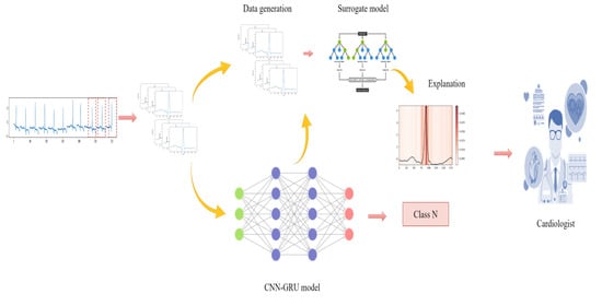
  • Proposing B-LIME as an improvement of the LIME method for generating a credible and meaningful explanation of ECG signal data, taking into account the signals’ temporal dependency, and comparing performance to LIME.
  • Proposing a data-generation technique that is locally faithful to the neighborhood of the prediction being explained to generate credible explanations.
  • Proposing an explanation method that simulates the reasonable accuracy of the original ML model and generates meaningful explanations.
  • Proposing a visual representation of LIME on the ECG dataset by applying a heatmap to highlight important areas on the heartbeat signal that the CNN-GRU mode uses for prediction.
  • Developing a hybrid 1D CNN-GRU model combining two powerful deep learning algorithms to classify four types of arrhythmias from ECG lead II.
The remainder of this article is structured as follows:
Section 2 reviews related work on optimizing LIME instability and discusses their proposed work. Section 3 explains the methods behind LIME and its functionality, including the B-LIME enhancement to generate credible and meaningful explanations for heartbeat signals. Section 4 shows a case study of cardiac arrhythmia classification using a hybrid CNN-GRU model. Section 5 discusses the results of the hybrid CNN-GRU model along with its prediction explanations that B-LIME generates and compares them with LIME explanations. Section 6 provides a conclusion and future direction for this work.

2. Related Work

The term interpretability and explainability in machine learning are widely gaining momentum in the literature. The various approaches to interpretability have been discussed in our previous review paper [9]. Post-hoc is a popular approach as it has the flexibility for the examination of a relationship or effect after the DL model has been trained [15].
It refers to any interpretation technique used to get insight from a trained machine learning model without affecting the model’s internal work. Post-hoc methods can be categorized into model-agnostic methods that can apply to any machine learning algorithms, such as LIME [11], SHAP [16], and anchors [17], and model-specific methods that are only applicable to specific machine learning algorithms, such as CAM [18], Grad-CAM [19], and Layer-Wise Relevance [20].
LIME [11] is a well-known, locally interpretable, model-agnostic explanation method. It trains a surrogate model to simulate a given ML model and explain its predictions. LIME artificially generates data points around the instance that need explanation using perturbation techniques and then trains a linear ML model to generate explanations. However, due to the linearity and random perturbation techniques that LIME employs to generate explanations, LIME suffers from some problems that influence its implementation in critical fields such as healthcare and finance. Therefore, many extensions have been proposed to tackle the problem of instability and linearity in LIME [21,22,23,24,25,26,27,28,29].
Guided-LIME [21] is a variant of LIME that aims to address the issues of instability and linearity in the original LIME method by introducing a Formal Concept Analysis (FCA) for the structured sampling of instances. FCA is a method used to analyze a training dataset to identify feature implication rules. These rules are then used to select appropriate samples for training a surrogate, explainable model.
OptiLIME [22] is a method for optimizing the LIME algorithm. It aims to improve the interpretability and stability of LIME using an optimization-based approach to find the best set of weights for the features in the explanation. Authors in OptiLIME highlight the trade-off between the LIME explanation’s stability and adherence and propose a framework that automatically finds the best kernel width that maximizes stability while retaining a predefined level of adherence.
ALIME [23] is an extension of LIME that provides modifications to improve the instability and local fidelity of LIME. To improve stability, ALIME generates a large number of data points in advance by sampling from a Gaussian distribution. To improve local fidelity, it employs an autoencoder technique to weight the local model, resulting in a more robust and accurate representation of the data.
MeLIME [24] is proposed to improve the local explanations of LIME, considering the dataset distribution of the DL model to generate meaningful explanations. MeLIME investigates four different types of data generation, namely Kernel Density Estimator (KDE), Principal Component Analysis (PCA), Variational Auto Encoder (VAE), and Word to Vector (Word2vec).
In K-LIME [25], the predictions of complex response functions are explained using local generalized linear model (GLM) surrogates. Instead of simulated or perturbed observation samples, local regions are defined by K clusters or segments that are chosen by the user. The input training data is separated into K disjoint sets using K clustering, which segments the local regions. Each cluster then applies a local general linear model, and the K is adjusted to maximize the R2 for all local models. LIME-SUP [26] is an improvement of K-LIME and replaces the unsupervised clustering technique used in K-LIME with a supervised partitioning tree to improve the explanations.
NormLIME [27] is a technique that combines and standardizes multiple local explanations to estimate the overall significance of all features used by the model. In NormLIME, the feature importance scores are calculated based on the difference between the model’s predicted class probabilities for the instance being explained and the neighborhood of the instance in the input space after normalizing the input features. This normalization helps to control for the scale of the input features and ensures that the feature importance scores are more representative of the model’s decision-making process.
DLIME [28] is a technique for explaining the predictions of machine learning models, particularly those used in computer-aided diagnosis systems. It is an extension of the LIME algorithm that addresses the lack of determinism in the explanations provided by LIME. In DLIME, instead of using random perturbation, DLIME employs agglomerative Hierarchical Clustering (HC) to group the training data and K-Nearest Neighbor (KNN) to identify the appropriate cluster for the instance being explained. Once the relevant cluster is identified, a linear model is trained on the selected cluster to produce explanations.
LIME-Aleph [29] aims to provide a more interpretable explanation for black-box classifiers by combining LIME and Automated Learning of Rules and Patterns (Aleph). It applies the Inductive Logic Programming approach Aleph to generate explanations in terms of logic rules to capture combinations of features and relations between the features. Aleph is a system for learning first-order rules from examples and has a powerful inference engine for searching for complex relational rules. The paper suggests that by combining LIME and Aleph, it is possible to approximate non-linear decisions with relational rules that may be more understandable for humans.
AudioLIME [10] is a technique for providing interpretable explanations for predictions made by audio-based machine learning models. It is an extension of LIME that uses source separation algorithms to provide listenable explanations from waveform-based predictions. It works by breaking down the audio signal into small segments and applying the LIME algorithm to these segments to provide explanations for the model’s predictions. The perturbations used in audioLIME are created by switching on/off components extracted by source separation to generate listenable explanations.
G-LIME [30] is a global-to-local method that first estimates global feature importance using a global prior and then explains the predictions for each instance locally by fitting a linear model to the most important features. The global prior is used to identify a subset of the data that can be closely related to the sample being explained. This subset is then analyzed in more granular detail, with the output providing a better understanding of the model’s behavior.
S-LIME [31] uses LIME and adds a stabilization algorithm to make the output results more reliable. S-LIME uses a statistical approach to ensure the stability of the explanations it generates by determining the number of perturbation points needed. It analyzes the Least Angle Regression (LARS) algorithm and quantifies the asymptotic statistics involved in selecting the next variable. With the help of a hypothesis testing procedure, S-LIME can automatically and adaptively determine the number of perturbations required to provide a stable explanation.
SurvLIME [32] framework is introduced as a modification of the LIME method. The central concept of the proposed methods involves using the Cox proportional hazards model to approximate the survival model in the vicinity of a test example. This choice is motivated by the fact that the Cox model considers a linear combination of example covariates, allowing for the coefficients of the covariates to be interpreted as having quantifiable impacts on the prediction. SurvLIME-Inf [33] is a modified version of the SurvLIME framework that is adapted to the characteristics of survival datasets. Specifically, this new methodology takes into account potential differences between the observed and predicted values.
In this work, comprehensive modifications to LIME functionality have been proposed to handle LIME instability and local fidelity limitations. B-LIME is an improvement of LIME that focuses mainly on generating meaningful explanations for ECG signal data taking into consideration the temporal dependencies between the features. Moreover, to ensure the credibility of the generated explanations, B-LIME proposes some modifications to LIME, including data generation techniques, explanation methods, and representation techniques.

3. Materials and Methods

3.1. LIME Explanation Technique

LIME is a surrogate model that creates an interpretable linear model over the main model that is locally faithful to the instance being explained (reference). First, it creates a new dataset of the original data point and the underlying model predictions by disturbing their features. It then trains an interpretable linear model weighted by the similarity of the perturbed dataset to the reference. Figure 1 presents the LIME procedure to generate explanations.
The functionality of LIME can be summarized as follows:
To explain a particular prediction x , LIME generates synthetic data Z around the prediction using the Gaussian sampling technique. The Gaussian sampling technique uses the mean and standard deviation of the reference distribution to generate a disturbing dataset from the parameterized normal distribution. However, this needs to include the correlation between features, which can lead to an unlikely and unrealistic dataset [21]. Then, LIME calls the black box model f to generate predictions y z for each instance in the disturbed dataset z in Z . To sample the disturbed dataset around the reference and ensure local fidelity, LIME uses the Euclidean distance metric π . The Euclidean distance metric weights the proximity of the disturbing instance by assigning higher weights to points closer to the reference π x ( z ) . This allows LIME to establish a local image of the decision area around the reference point. Feature selection is then performed to keep only the most important features and ensure the explanations’ understandability. However, due to the random perturbation generating the disturbed dataset, a slight change in the data can lead to significant changes in the selected feature subset [34]. Therefore, ignoring the stability problem of the feature selection algorithm may lead to the wrong explanation [35]. Finally, LIME trains a locally weighted ridge regression model g by fitting the disturbed dataset Z , the disturbed labels y z and the weights π z . The coefficients of the ridge regression model are used as explanations. To generate explanations, LIME uses the following formula:
ε ( x ) = a r g m u n g G ( f , g , π x ) + Ω ( g )
ε ( x ) is the interpretable model explanation, ( f , g , π x ) is the measurement of how unfaithful g is in imitating f in the locality π x , and Ω ( g ) is the measurement of the complexity of the local model g .

3.2. The Proposed B-LIME Technique

LIME has several packages that can provide explanations for various ML models. Moreover, LIME explanations mainly focus on two aspects: the ML algorithm and the type of dataset, i.e., tabular, texture, or image. Unfortunately, LIME does not have any packages to represent explanations of signal data. Therefore, the proposed B-LIME improves the LIME interpretation technique by providing explanations to signal data such as ECG arrhythmias. Figure 2 presents the B-LIME procedure to generate explanations.
B-LIME mainly focuses on generating credible and meaningful explanations for heartbeat signals, taking into consideration the temporal dependencies between features. Moreover, to ensure the credibility of the generated explanations, B-LIME proposes modifications to LIME, including the data generation technique, the explanation method, and the representation technique. Algorithm 1 represents the proposed B-LIME algorithm in pseudocode.
Algorithm 1: B-LIME pseudocode
I n p u t : E C G R e c o r d ( L 2 ) , W i n d o w s i z e ( w ) , S a m p l S i z e ( s ) , P r e d i c t i o n s ( p ) , M o d e l ( F )
Output: Explanations
Start Algorithm (B-LIME)
Phase 1, Split ECG record into heartbeats
1|     F u n c t i o n   H e a r t b e a t S p l i t ( L 2 , w ) :
2|                       I n i t i a l i z e   Q R S , h e a r t b e a t {   }
3|                       Q R S = L 2 . E x t r a c t Q r s P o s i t i o n s ( )
4|                       W h i l e ( p e a k   i n   Q R S ) d o
5|                                         s t a r t ,   e n d = p e a k w / / 2 ,   p e a k + w / / 2
6|                                         h e a r t b e a t . a p p e n d ( l 2 [ s t a r t : e n d ] )
7|                       e n d   W h i l e
8|                       R e t u r n   h e a r t b e a t
Phase 2, Bootstrapping resampling
9|     F u n c t i o n B o o t s t r a p ( H e a r t b e a t S p l i t   ( L 2 , w ) , S a m p l S i z e ( s ) ) :
10|                       I n i t i a l i z e b o o t s { }
11|                       F o r   i   f r o m   0   t o   s   d o
12|                                         i d x = random integer between 0 and l e n ( h e a r t b e a t )
13|                                         b o o t s . a p p e n d ( h e a r t b e a t [ i d x ] )
14|                       e n d   F o r
15|                       R e t u r n   b o o t s
Phase 3, Generate explanations
16|  Function RandomForest (data, p):
17|                       I n i t i a l i z e d a t a , f o r e s t , f e a t u r e s { }
18|                       l a b e l = F ( d a t a )
19|                       d a t a = c o n c a t e n a t e   ( B o o t s t r a p   ( H e a r t b e a t S p l i t   ( L 2 ,   w ) ,   S a m p l e S i z e   ( s ) ) ,   l a b e l )
20|                       n e i g h b o r h o o d = P a i r w i s e   d i s t a n c e   b e t w e e n   ( p , d a t a )
21|                       F o r   i   f r o m   0   t o   s   d o
22|                                         B o o t s t r a p p e d D a t a = B o o t s t r a p ( d a t a , 100 )
23|                                         t r e e = D e c i s i o n T r e e ( B o o t s t r a p p e d D a t a , n e i g h b o r h o o d )
24|                                         f o r e s t . a p p e n d ( t r e e )
25|                       e n d   F o r
26|                       f e a t u r e s = f o r e s t . F e a t u r I m p o r t a n t
27|                       e x p l a i n a t i o n = h e a t m a p   ( f e a t u r e s ,     c m a p = R e d s ,
                                                                  a s p e c t = a u t o , i n t e r p r e t a t i o n = n e a r t e s t ,
                                                                                                                      a l p h a = 0.5 )
28|                             P l o t   ( e x p l a i n a t i o n , p)
29End;//Algorithm
To compute the time complexity of the proposed B-LIME extension, we use asymptotic notations, namely big- O analysis. The easiest approach to comparing an algorithm’s time complexity is to determine how many basic (or dominating) operations the algorithm must perform to converge. This calculation may be conducted using the big O notation, which is a common representation of time complexity [36]. Evidently, the quantity of incoming data affects how many dominating processes are present [37].
When referring to an algorithm’s time complexity, we mean the relationship between the algorithm’s input size and the amount of time it takes to run. From this, we can see that B-LIME uses three operations. The first operation is to calculate the distance between the heartbeat being explained x and the generated dataset b X .
This operation runs ( n 2 ) times for all instances in the dataset b X except the instance being explained. The second operation calls the random forest algorithm to provide feature weight to the instance b X [ i ] . Random Forest is an ensemble model of decision trees that contains M treas. Biau [38] induct the time complexity of the random forest as follows:
M d n l o g ( n )
where M is the number of trees, d is the number of features and n is the number of instances in the dataset. The third operation is to call the heatmap for each instance and return the results. In the worst case, if the condition is always met, the total number of operations and therefore time complexity of B-LIME can be expressed as follows:
T ( n ) = 2 n 2 M d l o g ( n ) 4 n M d l o g ( n )  
The big O notation specifies the most dominant term in an algorithm’s time complexity and, therefore, the way its execution time is affected by changing the input size. Most times, instead of considering the whole equation of the complexity, we just keep the highest order term, as it usually dominates the rest, especially as the input size n grows. With all this previous information, we would say that the time complexity of the B-LIME algorithm is.
T ( n ) = 2 n 2 M d l o g ( n )  
From the previous equation, it is clear that the time complexity of B-LIME depends on the number of instances in the dataset   n , the number of trees in the random forest   M and the number of features each instance has d .

3.2.1. Data Generation

When generating disturbing data, time series data have special bonds between features that should be considered. However, as mentioned in Section 3.1., LIME generates random data points around the reference using the Gaussian sampling technique and ignores the correlation between features, resulting in unrealistic data points. To overcome these limitations, we propose a data generation technique that benefits from the ECG architecture and bootstrapping technique. Each ECG record generally contains a different number of heartbeats depending on time, frequency, and the patient’s heart rate. For example, record 100 from MIT-BIH is 30 min long, has a frequency of 360, and is segmented into 2271 heartbeats. Therefore, instead of using random perturbation techniques to generate data as in LIME, B-LIME segments the ECG record into heartbeats and then implements the bootstrapping technique to generate a resampling data point. Figure 3 illustrates the difference between the LIME and B-LIME perturbation techniques. As shown in the figure, the B-LIME is more faithfully localized to the neighborhood of the given instance (blue dot), and the generated data are more realistic to the original heartbeat.
Bootstrapping is a statistical method that involves resampling a sample with replacements to generate new data. This can be useful for a variety of purposes, including generating additional data for training machine learning models, constructing confidence intervals for sample statistics, and evaluating the stability and robustness of models [39]. One common use of bootstrapping for data generation is in the context of training machine learning models [40]. When working with a limited amount of data, it can be useful to artificially generate additional data by resampling the existing data. This can be done by selecting a random subset of the data, with the possibility of selecting the same data point multiple times, and then using this subset as a new “bootstrapped” sample. This process can be repeated multiple times to generate multiple bootstrapped samples [41]. The resampling approach offers unbiased estimates since it is based on random samples of all conceivable data outcomes [42].
One of the key advantages of the B-LIME data generation technique is that it takes into account the correlation between features in time series data. By segmenting the ECG record into heartbeats, the technique preserves the temporal dependencies between the ECG features, which leads to more realistic and informative data points compared to LIME’s random perturbation technique. Furthermore, B-LIME uses a statistical method called "bootstrapping," which involves resampling a sample with replacement in order to get new data. This technique is commonly used to generate additional data for training machine learning models and evaluating the stability and robustness of those models. By resampling the existing data with replacement, the bootstrapping technique generates new data points that are similar to the original data but not identical. This allows for a more thorough exploration of the underlying patterns and relationships in the data.
The B-LIME data generation technique is robust as it is based on random samples of all conceivable data outcomes, which offers unbiased estimates. As shown in Figure 3, the resampling approach provides more realistic and informative data points compared to other data LIME.

3.2.2. Explanations Generation
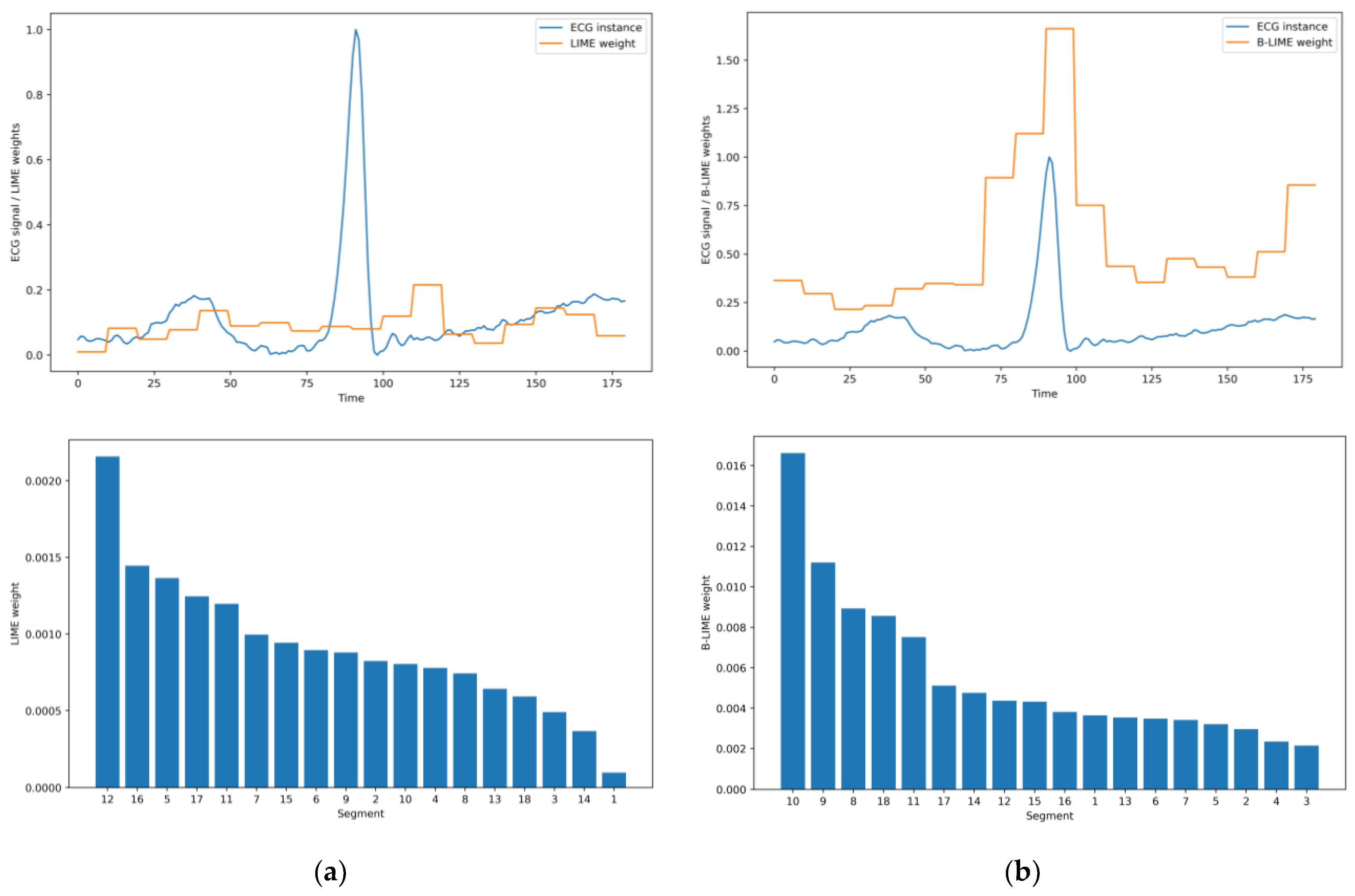
To generate explanations, LIME builds a ridge regression model and uses the coefficient to indicate the impact of each feature in the instance on the ML model. However, ridge regression assumes linear relationships between features, which is not the case in most situations. Moreover, it applies a penalty throughout the estimation process that is proportional to the standard deviation of the coefficient. Ridge regression can be helpful with a high-variance dataset that is not locally faithful to the original data. However, if the data are locally faithful, the ridge regression penalty can be detrimental, distorting the exact parameter values and leading to unstable explanations [22]. Therefore, we propose Random Forest.
Random Forest (RF) is a machine learning algorithm that is easy to use, scalable, and produces good results for both linear and non-linear relationships without requiring hyper-parameter tuning [43]. It consists of a collection of Decision Trees (DTs) that are slightly different from each other and implicitly perform feature selection to create uncorrelated decision trees [44]. RF works by performing the following steps: (1) creating a bootstrapped dataset by randomly selecting, with replacement, samples from the original dataset; (2) training a decision tree on the bootstrapped dataset, but only using a random subset of features at each step; and (3) repeating these steps 100 times and making a final classification based on averaging the predictions of all the individual decision trees [45,46]. RF is preferred over LIME Ridge Regression because it can handle both linear and non-linear relationships between features without requiring hyper-parameter tuning. It also provides a variable importance measure and is easy to interpret. RF is different from ridge regression in that it is a set of decision trees that automatically select features. This makes it resistant to noisy data and eliminates the need for cross-validation [43]. Figure 4 compares the feature importance generated by LIME and B-LIME.
One of the advantages of random forests is that they are relatively easy to interpret compared to some other machine-learning models. This is because the decision trees in a random forest are individually interpretable, and the final prediction of the random forest can be traced back to the individual decision trees [47]. Another way to interpret a random forest is to look at the importance of the features. Many implementations of random forests provide a feature importance measure, which tells you how important each feature is in making predictions [48]. This can help identify the most important features in the model and understand how they contribute to the final prediction.

3.2.3. Heatmap

A heatmap is a graphical representation of data that can be used to visualize the relationships between variables and identify patterns or correlations in the data [49]. Heatmaps are often used in machine learning to visualize the results of different algorithms or models. Heatmaps can be used to identify patterns or trends in the data that may not be immediately obvious when looking at the raw data. For example, a heatmap might be used to visualize the correlations between different features in a dataset or to identify areas where an algorithm is performing particularly well or poorly. Heatmaps can be a useful tool for interpreting machine learning models and understanding how they are making decisions. In this research, the use of heatmaps to improve B-LIME explainability can be summarized as follows:
  • Identifying feature importance: Heatmaps can be used to visualize the importance of different features in a model. This can help you understand which features are most influential in the model’s predictions and can inform feature selection or feature engineering efforts.
  • Explaining model predictions: Heatmaps can be used to visualize the relationships between different features and the model’s predictions. This can help to understand how the model uses different features to make predictions and can provide insight into the model’s decision-making process.
Heatmaps can be used to visualize the importance of different features in a model, the relationships between different features, and the model’s predictions. This information can inform feature selection or feature engineering efforts and provide insight into how the model uses different features to make predictions. Overall, heatmaps can be a useful tool for improving the interpretability of machine learning models and understanding how they are making decisions.

4. Case Study

To validate the B-LIME explanation, we use the well-known MIT-BIH dataset [50]. It has been employed for cardiac arrhythmia classification from ECG signals. Moreover, we develop a hybrid deep learning model, CNN-GRU, to classify four types of arrhythmias. The aim is to validate the B-LIME explanations and compare them to LIME. Figure 5 presents the schematic pipeline of the study.

4.1. Data Preparation

In this work, the ECG lead II obtained from the MIT-BIH [50] dataset is used as a data source to classify four arrhythmias according to the Association for the Advancement of Medical Instrumentation (AAMI) standard EC57. The MIT-BIH dataset contains 48 ECG recordings of a half-hour-long obtained from 47 patients. Each record has two types of ECG signals: lead II and lead V5. The recordings were digitally converted to 360 samples per second per channel with an 11-bit precision across a 10-mV range. To classify arrhythmias, the 48 records were extracted and segmented into heartbeats with a length of 180. The heartbeat signal is centered on the R-peak point to ensure that all the important features such as the QRS complex, P-wave, and T-wave are extracted correctly. Moreover, all the extracted beats have identical lengths, which is essential for training the model.
After segmenting the signals into heartbeats, the total number of heartbeats is 107,775 for the 48 records. The number of heartbeats for each class differs from one to another. The heartbeats are categorized into 89,694 for normal beats, 6487 for ventricular ectopic beats, 2814 for supraventricular ectopic beats, 779 for fusion beats, and 24 for unknown beats. The unknown beats have dropped because they contain unclassified beats [51]. The dataset has been split into 75 percent training and 25 percent testing. We used the stratify parameter to ensure that all the classes had been split equally into the training and testing data.
After checking the sample size of each class in the training dataset, we found a significant imbalance among the four classes (i.e., class ‘N’ has 67,270, while class ‘F’ has only 584). Therefore, a resampling technique was applied to the training data to remove the imbalance between the classes and reduce overfitting. Unbalanced classes affect the sensitivity of the model to the minority classes [52]. Therefore, a downsampling method is applied to class ‘N’ to reduce the number of samples from 67,270 to 25,000 since it is the majority class. An upsampling method is applied to the remaining classes ‘S’, ‘V’, and ‘F’ to increase the number of samples to 25,000, as they are the minority classes. The test data is kept unchanged to prevent data leakage, which might lead to overfitting.

4.2. Training Classification Model

Two DL network algorithms (CNN-GRU) are combined into a single model to classify four classes of cardiac arrhythmias based on ECG lead II. CNNs are well-suited for processing and analyzing data that has a grid-like structure, such as images [53]. They can automatically learn features from the input data and are particularly effective at identifying patterns and features that are important for the task at hand [54].
GRUs are a type of recurrent neural network (RNN) that are designed to handle sequential data, such as time series or natural language [55]. They have a gating mechanism that allows them to selectively retain or forget information from the past, which helps them to model long-term dependencies in the data [56].
By combining the strengths of CNNs and GRUs, a 1D-CNN-GRU network can process both grid-like and sequential data. This makes it a powerful tool for tasks such as natural language processing [57], speech recognition [58], and time series forecasting [59].
The proposed hybrid model architecture contains two 1D CNN layers to extract relationships between features and a GRU layer to support sequence feature extraction. The output of the GRU layer is passed to a fully connected layer of four dense layers to classify four types of arrhythmias.
1D-CNN is an alternative, modified version of CNN designed for 1D signals, especially sparse data that is not suitable for traditional CNN [60]. Due to its compact and simple configuration and performance, 1D-CNN is also suitable for real-time applications and low-cost hardware implementations [13].
GRU is an improved version of RNN designed to solve the vanishing that occurs in RNN during backpropagation. GRU has shown improvements in several applications, including sequential and time-serial data [61]. The internal mechanisms (gates) of GRU can regulate the flow of information to learn which data in a sequence is important to keep. The GRU contains two gates: a reset gate r to manage the addition of new input to the existing memory and an update gate z to regulate memory retention [62].
A hybrid model of 1D CNN and GRU can provide a posterior probability that the input sequence contains arrhythmias and achieve higher classification accuracy [63]. Figure 5 shows the architecture of the proposed hybrid 1D CNN-GRU model. 1D CNN can efficiently extract important features and reduce the computational cost. However, it has some limitations on sequential and time-series data as it requires some kind of memory performance [64]. On the other hand, GRU performs well on such data because its internal mechanisms can learn which data in the sequence is essential to keep. However, GRU is time-consuming and computationally intensive. Therefore, proposing a hybrid model that combines these two algorithms, 1D CNN and GRU, can improve the performance of the model, reduce computational costs, and improve sequence prediction.

4.3. Experiments Setup

The experiment was implemented using the Python programming language on the Anaconda platform. The Sklearn and TensorFlow libraries were used to build and evaluate the model, and the LIME library was used to employ LIME.
An intensive experiment was conducted to select the minimal model architecture with optimal parameters to improve the model’s performance and reduce training time. We believe that if the model has a great performance, that will lead to better explanation outcomes. The architecture of the proposed hybrid model consists of two blocks for CNN and another block for GRU. Each CNN block consists of one CNN layer along with a Max-pooling layer, a Dropout layer, and a Batch-normalization layer. The Max-pooling layer calculates the maximum or largest value in each patch of each feature map to down sample the feature maps to highlight the most present feature in the patch. The Dropout layer of 0.20 and the normalization layer were applied to reduce overfitting [65]. The Dropout layer randomly sets inputs to zero with a frequency of rate at each step during training time. The Batch-normalization layer normalize the inputs in a layer for each mini-batch, ensuring a fast and stable learning process [66]. In this experiment, each 1D CNN layer has 64 filters with a kernel size of five to define the window length and ReLU as the activation function. Table 1 summarizes the tuning parameters of the proposed hybrid model.
The GRU block contains one GRU layer along with one Max-pooling layer and one Batch-normalization layer. The GRU layer is trained with 64 memory units for each input of the sequence, vertically attached to each other, and each one passes the filtered information to the next memory unit. A fully connected layer contains four dense cells, and a SoftMax activation function was added to categorize the output of the three models into the four arrhythmia classes. The sparse cross-entropy is applied to the loss function, and the Adam optimizer with a learning rate of 0.001 and a decay factor of 1 × 10⁻⁶ is used to train the three models. The model fits the training and validation datasets with a batch size of 512 for 100 epochs. The training times of the models were 3, 72, and 8 s per epoch for 1D CNN, GRU, and 1D CNN-GRU, respectively, on a GeForce GTX 1070 processor.

5. Results and Discussion

This section presents and analyzes the results obtained from applying B-LIME to a deep learning model (CNN-GRU) for classifying cardiac arrhythmias and compares the results with those obtained using LIME. The main objective of this study is to demonstrate that B-LIME can effectively improve the explainability of deep learning models for ECG data by considering the temporal dependencies between the ECG features. It is widely recognized that the accuracy of a model is a critical factor for its interpretability and the ability to make informed decisions based on its predictions. In light of this, we have proposed the use of the CNN-GRU model for classifying arrhythmias, as it offers a high degree of accuracy and the potential to produce reliable results.
In the following section, the CNN-GRU model’s results are analyzed in detail, including their accuracy and other performance metrics such as the confusion matrix parameters. We will then apply B-LIME to provide explanations and compare its results with those obtained using LIME. We aim to provide a comprehensive evaluation of the effectiveness of B-LIME in improving the explainability of deep learning models for ECG data.

5.1. CNN-GRU Model

The CNN-GRU model benefits from CNN’s ability to extract features, learn locally related data, and reduce computational costs, as well as GRU’s ability to capture features from data-related time series. Unlike the standalone model that can only capture partial relationships between features, the combinations of 1D CNN and GRU algorithms can model the complex relationships between ECG signals and cardiac arrhythmias. Table 2 describes the CNN-GRU performance in the training and testing datasets.
As can be seen from Table 3, the model has perfect scores in all performance metrics with a minimum loss of 0.02 in the training dataset. In the testing dataset, the model still scores an adequate performance in all metrics except precision and F1-score of class F, in which the model scores 0.72 and 0.78, respectively.
Moreover, the confusion matrix for each class of training and testing datasets, as shown in Figure 6, indicates the percentage of correctly predicted samples against incorrectly predicted samples for each class. For instance, 0.86 percent of the 195 cases in class F are correctly classified, whereas 0.10 percent and 0.04 percent, respectively, are incorrectly classified as classes N and V.
It is important to note that the CNN-GRU model has a slight bias towards class N, as shown by the confusion matrix. This bias is shown clearly in class F with 0.10 percent, followed by classes S and V with 0.08 and 0.03 percent, respectively. This bias is not important here since our main goal is to explain the model’s performance with B-LIME and compare it to LIME.

5.2. B-LIME Technique

To enhance LIME explanations on signal data, B-LIME introduced modifications to LIME in three aspects, including data generation, explanation algorithm, and representation technique.
As mentioned in Section 3, LIME suffers from explanation instability and local fidelity. The main reason for LIME instability is the data generation technique that randomly perturbs the instance features to generate a dataset. Thus, every time LIME is called, new data points are generated that might be different from the previous ones. Moreover, the broad definition of the neighborhood around the instance being explained is the main reason why LIME suffers from local fidelity [24]. B-LIME tackles the above-mentioned limitations of LIME by proposing a new data generation technique that benefits from the ECG signal’s nature and bootstrapping method. As can be seen from Figure 3., the B-LIME data generation technique ensures that each data point is locally faithful to the original dataset. Moreover, the B-LIME data generation technique does not affect the temporal dependencies between time-series features that lead to credible explanations. Figure 4 illustrates the difference between LIME and B-LIME explanation outcomes. In the context of arrhythmia classification, the QRS complex provides valuable information about the electrical activity of the heart and helps to differentiate between different types of arrhythmias. Furthermore, the QRS complex is also used as a reference point for measuring other ECG parameters, such as the PR interval, which represents the time between the start of atrial depolarization and the start of ventricular depolarization. By analyzing the QRS complex, along with other ECG parameters, it is possible to classify different types of arrhythmias and make more informed decisions about patient care and treatment.
To gain an understanding of the results, we calculated the average weight of the results for a sequence of eighteen time points, where each point represents 10% of the heartbeat features. This allowed us to gain interpretability from ten slices. Figure 7 provides examples of the explanations obtained from both LIME and B-LIME. The figure shows the sorted weights per slice of LIME and B-LIME, with slice ten scoring the highest weight in B-LIME, followed by slice nine. These two slices represent the QRS complex. In addition, the figure displays the weights (multiplied by 100 for better visibility) along with the instance being explained. It can be observed that in B-LIME, the slice with the QRS complex has the most significant weight, while in LIME, different areas are selected randomly.
In the real world, the QRS complex is a critical area in the diagnosis of a wide range of cardiac pathologies, including arrhythmias [67], which support B-LIME representation.
Moreover, in Figure 8, the heatmap lightness bar shows that B-LIME is more confident about the feature selected compared to LIME, where the lower feature of B-LIME has an important score of 0.01, which is the highest score in LIME. The main cause of LIME randomly selecting areas is the perturbation of the feature, which confuses the model instead of helping it recognize important areas in the signal. Figure 7 compares B-LIME explanations to the four classes with LIME explanations. As can be seen from the figure, B-LIME usually highlights the area between 75 and 110 to distinguish between classes and categorize arrhythmias, which is most likely the QRS complex area.

5.3. Significance Analysis

The one-way analysis of variance (ANOVA) test is a statistical method used to determine if there is a significant difference between the means of multiple groups. It is a hypothesis-testing technique that compares the means of two or more independent groups to determine if there is evidence to reject the null hypothesis that the group means are equal. The null hypothesis states that there is no significant difference between the proposed B-LIME and existing LIME algorithms. If the p-value is larger than 0.05, the null hypothesis is considered true, while a p-value less than 0.05 means it is rejected [68]. The ANOVA test was utilized to determine the statistical significance of the improvement obtained by the B-LIME method compared to the traditional LIME approach. Results from the test, as depicted in Table 3, demonstrate that the calculated p-value of 8.544500 × 10⁻³⁵ indicates a rejection of the null hypothesis and provides evidence of a significant difference between the two methods. Additionally, the differences are further illustrated through the use of a box plot in Figure 9, which visually displays the distribution of the significant differences between B-LIME and LIME. The utility of the proposed B-LIME method can be demonstrated through the visual representation presented in Figure 7. This illustration effectively emphasizes the crucial areas that are typically utilized by medical professionals in the classification of cardiac arrhythmias.

6. Conclusions

In this paper, we propose a B-LIME technique that improves LIME to explain signal data, taking into account the temporal dependence between time series features. Moreover, B-LIME enhances LIME explanations by considering three aspects, including data generation technique, explanation method, and representation technique to ensure credible and meaningful explanations. The B-LIME explanations were examined in a proposed hybrid CNN-GRU model for cardiac arrhythmia prediction and compared with LIME explanations. In comparison to LIME, which highlights random areas, B-LIME performs well in highlighting key areas that physicians normally use to diagnose cardiac arrhythmias, such as the QRS complex. In future work, we intend to dive deeper and investigate the question of why the model classifies a prediction as class A but not class B. Moreover, we will investigate B-LIME on a more signal-based model and evaluate its performance compared to LIME.

Author Contributions

Conceptualization, T.A.A.A. and M.S.M.Z.; methodology, T.A.A.A. and M.S.M.Z.; software, T.A.A.A.; validation, T.A.A.A., M.S.M.Z. and W.A.; formal analysis, T.A.A.A.; investigation T.A.A.A.; resources, T.A.A.A. and S.U.H.; data curation, T.A.A.A.; writing—original draft preparation, T.A.A.A.; writing—review and editing, T.A.A.A.; visualization, T.A.A.A.; supervision, M.S.M.Z. and W.A.; project administration, M.S.M.Z.; funding acquisition, M.S.M.Z. All authors have read and agreed to the published version of the manuscript.

Funding

This research has been supported by the Yayasan Universiti Teknologi PETRONAS Fundamental Research Grant (YUTP-FRG) under Grant 015LC0-244.

Data Availability Statement

The MIT-BIH Arrythmia Database is available in physionet.org website.

Conflicts of Interest

The authors declare no conflict of interest.

References

  1. Hu, H.; Zhang, Z.; Xie, Z.; Lin, S. Local Relation Networks for Image Recognition. In Proceedings of the IEEE/CVF International Conference on Computer Vision, Seoul, Republic of Korea, 27 October–2 November 2019. [Google Scholar]
  2. Abdel-Hamid, O.; Mohamed, A.-R.; Jiang, H.; Deng, L.; Penn, G.; Yu, D. Convolutional Neural Networks for Speech Recognition. IEEE/ACM Trans. Audio Speech Lang. Process. 2014, 22, 1533–1545. [Google Scholar] [CrossRef] [Green Version]
  3. Chowdhary, K.R. Natural Language Processing. In Fundamentals of Artificial Intelligence; Springer: Berlin/Heidelberg, Germany, 2020; pp. 603–649. [Google Scholar]
  4. Abdullah, T.A.; Ali, W.; Malebary, S.; Ahmed, A.A. A Review of Cyber Security Challenges Attacks and Solutions for Internet of Things Based Smart Home. Int. J. Comput. Sci. Netw. Secur 2019, 19, 139. [Google Scholar]
  5. Abdullah, T.A.A.; Ali, W.; Abdulghafor, R. Empirical Study on Intelligent Android Malware Detection Based on Supervised Machine Learning. Int. J. Adv. Comput. Sci. Appl. 2020, 11, 215–225. [Google Scholar] [CrossRef]
  6. Kiranyaz, S.; Ince, T.; Gabbouj, M. Real-Time Patient-Specific Ecg Classification by 1-D Convolutional Neural Networks. IEEE Trans. Biomed. Eng. 2016, 63, 664–675. [Google Scholar] [CrossRef] [PubMed]
  7. Alkhodari, M.; Fraiwan, L. Convolutional and Recurrent Neural Networks for the Detection of Valvular Heart Diseases in Phonocardiogram Recordings. Comput. Methods Programs Biomed. 2021, 200, 105940. [Google Scholar] [CrossRef] [PubMed]
  8. London, A.J. Artificial Intelligence and Black-Box Medical Decisions: Accuracy Versus Explainability. Hastings Cent. Rep. 2019, 49, 15–21. [Google Scholar] [CrossRef]
  9. Abdullah, T.A.A.; Zahid, M.S.M.; Ali, W. A Review of Interpretable Ml in Healthcare: Taxonomy, Applications, Challenges, and Future Directions. Symmetry 2021, 13, 2439. [Google Scholar] [CrossRef]
  10. Haunschmid, V.; Manilow, E.; Widmer, G. Audiolime: Listenable Explanations Using Source Separation. Expert Rev. Cardiovasc. Ther. 2020, 18, 77–84. [Google Scholar]
  11. Ribeiro, M.T.; Singh, S.; Guestrin, C. Why Should I Trust You? Explaining the Predictions of Any Classifier. In Proceedings of the 22nd ACM SIGKDD International Conference on Knowledge Discovery and Data Mining, San Francisco, CA, USA, 13–17 August 2016. [Google Scholar]
  12. Neves, I.; Folgado, D.; Santos, S.; Barandas, M.; Campagner, A.; Ronzio, L.; Cabitza, F.; Gamboa, H. Interpretable Heartbeat Classification Using Local Model-Agnostic Explanations on Ecgs. Comput. Biol. Med. 2021, 133, 104393. [Google Scholar] [CrossRef]
  13. Ahmed, A.A.; Ali, W.; Abdullah, T.A.; Malebar, S.Y. Classifying Cardiac Arrhythmia from Ecg Signal Using 1d Cnn Deep Learning Model. Mathematics 2023, 11, 562. [Google Scholar] [CrossRef]
  14. Ul Hassan, S.; Zahid, M.S.M.; Abdullah, T.A.A.; Husain, K. Classification of Cardiac Arrhythmia Using a Convolutional Neural Network and Bi-Directional Long Short-Term Memory. Digital Health 2022, 8, 20552076221102766. [Google Scholar] [CrossRef] [PubMed]
  15. Ayano, Y.M.; Schwenker, F.; Dufera, B.D.; Debelee, T.G. Interpretable Machine Learning Techniques in Ecg-Based Heart Disease Classification: A Systematic Review. Diagnostics 2022, 13, 111. [Google Scholar] [CrossRef] [PubMed]
  16. Lundberg, S.M.; Lee, S.-I. A Unified Approach to Interpreting Model Predictions. In Proceedings of the Advances in Neural Information Processing Systems, Long Beach, CA, USA, 4–9 December 2017. [Google Scholar]
  17. Ribeiro, M.T.; Singh, S.; Guestrin, C. Anchors: High-Precision Model-Agnostic Explanations. In Proceedings of the AAAI, Palo Alto, CA, USA, 26–28 March 2018. [Google Scholar]
  18. Zhou, B.K.; Lapedriza, A.; Oliva, A.; Torralba, A. Learning Deep Features for Discriminative Localization. In Proceedings of the IEEE Conference on Computer Vision and Pattern Recognition, Las Vegas, NV, USA, 27–30 June 2016. [Google Scholar]
  19. Selvaraju, R.R.; Cogswell, M.; Das, A.; Vedantam, R.; Parikh, D.; Batra, D. Grad-Cam: Visual Explanations from Deep Networks Via Gradient-Based Localization. In Proceedings of the IEEE International Conference on Computer Vision, Venice, Italy, 22–29 October 2017. [Google Scholar]
  20. Bach, S.; Binder, A.; Montavon, G.; Klauschen, F.; Müller, K.-R.; Samek, W. On Pixel-Wise Explanations for Non-Linear Classifier Decisions by Layer-Wise Relevance Propagation. PLoS ONE 2015, 10, e0130140. [Google Scholar] [CrossRef] [PubMed] [Green Version]
  21. Sangroya, A.; Rastogi, M.; Anantaram, C.; Vig, L. Guided-Lime: Structured Sampling Based Hybrid Approach Towards Explaining Blackbox Machine Learning Models. In Proceedings of the CIKM (Workshops), Galway, UK, 19–23 October 2020. [Google Scholar]
  22. Visani, G.; Bagli, E.; Chesani, F. Optilime: Optimized Lime Explanations for Diagnostic Computer Algorithms. arXiv 2020, arXiv:2006.05714. [Google Scholar]
  23. Shankaranarayana, S.M.; Runje, D. Alime: Autoencoder Based Approach for Local Interpretability. In Proceedings of the International Conference on Intelligent Data Engineering and Automated Learning, Guimaraes, Portugal, 4–6 November 2020. [Google Scholar]
  24. Botari, T.; Hvilshøj, F.; Izbicki, R.; de Carvalho, A.C.P.L.F. Melime: Meaningful Local Explanation for Machine Learning Models. arXiv 2020, arXiv:2009.05818. [Google Scholar]
  25. Hall, P.; Gill, N.; Kurka, M.; Phan, W. Machine Learning Interpretability with H2O Driverless AI. 2017. Available online: https://docs.h2o.ai/driverless-ai/latest-stable/docs/booklets/MLIBooklet.pdf (accessed on 13 February 2023).
  26. Hu, L.; Chen, J.; Nair, V.N.; Sudjianto, A. Locally Interpretable Models and Effects Based on Supervised Partitioning (Lime-Sup). arXiv 2018, arXiv:1806.00663. [Google Scholar]
  27. Ahern, I.; Noack, A.; Guzman-Nateras, L.; Dou, D.; Li, B.; Huan, J. Normlime: A New Feature Importance Metric for Explaining Deep Neural Networks. arXiv 2019, arXiv:1909.04200. [Google Scholar]
  28. Zafar, M.R.; Khan, N.M. Dlime: A Deterministic Local Interpretable Model-Agnostic Explanations Approach for Computer-Aided Diagnosis Systems. arXiv 2019, arXiv:1906.10263. [Google Scholar]
  29. Rabold, J.; Siebers, M.; Schmid, U. Explaining Black-Box Classifiers with Ilp–Empowering Lime with Aleph to Approximate Non-Linear Decisions with Relational Rules. In Proceedings of the International Conference on Inductive Logic Programming, Ferrara, Italy, 2–4 September 2018. [Google Scholar]
  30. Li, X.; Xiong, H.; Li, X.; Zhang, X.; Liu, J.; Jiang, H.; Chen, Z.; Dou, D. G-Lime: Statistical Learning for Local Interpretations of Deep Neural Networks Using Global Priors. Artif. Intell. 2023, 314, 103823. [Google Scholar] [CrossRef]
  31. Zhou, Z.; Hooker, G.; Wang, F. S-Lime: Stabilized-Lime for Model Explanation. In Proceedings of the 27th ACM SIGKDD Conference on Knowledge Discovery & Data Mining, Virtual, 14–18 August 2021. [Google Scholar]
  32. Kovalev, M.S.; Utkin, L.V.; Kasimov, E.M. Survlime: A Method for Explaining Machine Learning Survival Models. Knowl.-Based Syst. 2020, 203, 106164. [Google Scholar] [CrossRef]
  33. Utkin, L.V.; Kovalev, M.S.; Kasimov, E.M. Survlime-Inf: A Simplified Modification of Survlime for Explanation of Machine Learning Survival Models. arXiv 2020, arXiv:2005.02387. [Google Scholar]
  34. Nogueira, S.; Sechidis, K.; Brown, G. On the Stability of Feature Selection Algorithms. J. Mach. Learn. Res. 2017, 18, 6345–6398. [Google Scholar]
  35. Khaire, U.M.; Dhanalakshmi, R. Stability of Feature Selection Algorithm: A Review. J. King Saud Univ. Comput. Inf. Sci. 2019, 34, 1060–1073. [Google Scholar] [CrossRef]
  36. Sagheer, A.; Zidan, M.; Abdelsamea, M.M. A Novel Autonomous Perceptron Model for Pattern Classification Applications. Entropy 2019, 21, 763. [Google Scholar] [CrossRef] [PubMed] [Green Version]
  37. Ou, G.; Murphey, Y.L. Multi-Class Pattern Classification Using Neural Networks. Pattern Recognit. 2007, 40, 4–18. [Google Scholar] [CrossRef]
  38. Biau, G. Analysis of a Random Forests Model. J. Mach. Learn. Res. 2012, 13, 1063–1095. [Google Scholar]
  39. Bertolini, R.; Finch, S.J.; Nehm, R.H. Quantifying Variability in Predictions of Student Performance: Examining the Impact of Bootstrap Resampling in Data Pipelines. Comput. Educ. Artif. Intell. 2022, 3, 00067. [Google Scholar] [CrossRef]
  40. Tibshirani, R.J.; Efron, B. An Introduction to the Bootstrap; Monographs on Statistics and Applied Probability; Imprint Chapman and Hall/CRC: New York, NY, USA, 1993; Volume 57. [Google Scholar]
  41. Davison, A.C.; Hinkley, D.V. Bootstrap Methods and Their Application; Cambridge University Press: Cambridge, UK, 1997. [Google Scholar]
  42. Dixon, P.M. Bootstrap Resampling. In Encyclopedia of Environmetrics; Wiley: Hoboken, NJ, USA, 2006. [Google Scholar]
  43. Abdulkareem, N.M.; Abdulazeez, A.M. Machine Learning Classification Based on Radom Forest Algorithm: A Review. Int. J. Sci. Bus. 2021, 5, 128–142. [Google Scholar]
  44. Abdullah, T.A.A.; Zahid, M.S.B.M.; Tang, T.B.; Ali, W.; Nasser, M. Explainable Deep Learning Model for Cardiac Arrhythmia Classification. In Proceedings of the International Conference on Future Trends in Smart Communities (ICFTSC), Kuching, Sarawak, Malaysia, 1–2 December 2022; pp. 87–92. [Google Scholar] [CrossRef]
  45. Denisko, D.; Hoffman, M.M. Classification and Interaction in Random Forests. Proc. Natl. Acad. Sci. USA 2018, 115, 1690–1692. [Google Scholar] [CrossRef] [Green Version]
  46. Utkin, L.V.; Kovalev, M.S.; Coolen, F.P.A. Imprecise Weighted Extensions of Random Forests for Classification and Regression. Appl. Soft Comput. 2020, 92, 106324. [Google Scholar] [CrossRef]
  47. Liu, B.; Wei, Y. Interpreting Random Forests. J. Chem. Inf. Model. 2015, 55, 1362–1372. [Google Scholar]
  48. Zhang, J.; Wang, J. A Comprehensive Survey on Interpretability of Machine Learning Models. ACM Comput. Surv. CSUR 2018, 51, 93. [Google Scholar]
  49. Simonyan, K.; Vedaldi, A.; Zisserman, A. Deep inside Convolutional Networks: Visualising Image Classification Models and Saliency Maps. arXiv 2013, arXiv:1312.6034. [Google Scholar]
  50. Moody, G.B.; Mark, R.G. Mit-Bih Arrhythmia Database. 1992. Available online: physionet.org (accessed on 9 January 2023).
  51. Gai, N.D. Ecg Beat Classification Using Machine Learning and Pre-Trained Convolutional Neural Networks. arXiv 2022, arXiv:2207.06408. [Google Scholar]
  52. Ege, H. How to Handle Imbalance Data and Small Training Sets in Ml. 2020. Available online: towardsdatascience.com (accessed on 9 January 2023).
  53. Krizhevsky, A.; Sutskever, I.; Hinton, G.E. Imagenet Classification with Deep Convolutional Neural Networks. Commun. ACM 2017, 60, 84–90. [Google Scholar] [CrossRef] [Green Version]
  54. LeCun, Y.; Bengio, Y.; Hinton, G. Deep Learning. Nature 2015, 521, 436–444. [Google Scholar] [CrossRef] [PubMed]
  55. Chung, J.; Gulcehre, C.; Cho, K.; Bengio, Y. Empirical Evaluation of Gated Recurrent Neural Networks on Sequence Modeling. arXiv 2014, arXiv:1412.3555. [Google Scholar]
  56. Graves, A.; Graves, A. Long Short-Term Memory. In Supervised Sequence Labelling with Recurrent Neural Networks; Springer: Berlin/Heidelberg, Germany, 2012; pp. 37–45. [Google Scholar]
  57. Chen, Y. Convolutional Neural Network for Sentence Classification. Master’s Thesis, University of Waterloo, Waterloo, ON, Canada, 2015. [Google Scholar]
  58. Chan, W.; Park, D.; Lee, C.; Zhang, Y.; Le, Q.; Norouzi, M. Speechstew: Simply Mix All Available Speech Recognition Data to Train One Large Neural Network. arXiv 2021, arXiv:2104.02133. [Google Scholar]
  59. Nweke, H.F.; Teh, Y.W.; Al-Garadi, M.A.; Alo, U.R. Deep Learning Algorithms for Human Activity Recognition Using Mobile and Wearable Sensor Networks: State of the Art and Research Challenges. Expert Syst. Appl. 2018, 105, 233–261. [Google Scholar] [CrossRef]
  60. Kiranyaz, S.; Avci, O.; Abdeljaber, O.; Ince, T.; Gabbouj, M.; Inman, D.J. 1d Convolutional Neural Networks and Applications: A Survey. Mech. Syst. Signal Process. 2021, 151, 107398. [Google Scholar] [CrossRef]
  61. Dey, R.; Salem, F.M. Gate-Variants of Gated Recurrent Unit (Gru) Neural Networks. In Proceedings of the 2017 IEEE 60th International Midwest Symposium on Circuits and Systems (MWSCAS), Boston, MA, USA, 6–9 August 2017. [Google Scholar]
  62. Zhao, R.; Wang, D.; Yan, R.; Mao, K.; Shen, F.; Wang, J. Machine Health Monitoring Using Local Feature-Based Gated Recurrent Unit Networks. IEEE Trans. Ind. Electron. 2018, 65, 1539–1548. [Google Scholar] [CrossRef]
  63. Andersen, R.S.; Peimankar, A.; Puthusserypady, S. A Deep Learning Approach for Real-Time Detection of Atrial Fibrillation. Expert Syst. Appl. 2019, 115, 465–473. [Google Scholar] [CrossRef]
  64. Guo, L.; Sim, G.; Matuszewski, B. Inter-Patient Ecg Classification with Convolutional and Recurrent Neural Networks. Biocybern. Biomed. Eng. 2019, 39, 868–879. [Google Scholar] [CrossRef] [Green Version]
  65. Srivastava, N.; Hinton, G.; Krizhevsky, A.; Sutskever, I.; Salakhutdinov, R. Dropout: A Simple Way to Prevent Neural Networks from Overfitting. J. Mach. Learn. Res. 2014, 15, 1929–1958. [Google Scholar]
  66. Brownlee, J. A Gentle Introduction to Batch Normalization for Deep Neural Networks. 2019. Available online: https://machinelearningmastery.com/batch-normalization-for-training-of-deep-neural-networks/#:~:text=Batch%20normalization%20is%20a%20technique,required%20to%20train%20deep%20networks (accessed on 13 February 2023).
  67. Curtin, A.E.; Burns, K.V.; Bank, A.J.; Netoff, T.I. Qrs Complex Detection and Measurement Algorithms for Multichannel Ecgs in Cardiac Resynchronization Therapy Patients. IEEE J. Transl. Eng. Health Med. 2018, 6, 1900211. [Google Scholar] [CrossRef]
  68. Shutari, H.; Saad, N.; Nor, N.B.M.; Tajuddin, M.F.N.; Alqushaibi, A.; Magzoub, M.A. Towards Enhancing the Performance of Grid-Tied Vswt Via Adopting Sine Cosine Algorithm-Based Optimal Control Scheme. IEEE Access 2021, 9, 139074–139088. [Google Scholar] [CrossRef]
Figure 1. LIME procedure to generate explanations.
Processes 11 00595 g001
Figure 2. B-LIME procedure to generate explanations.
Processes 11 00595 g002
Figure 3. Data Generation Techniques.
Processes 11 00595 g003
Figure 4. Comparison between LIME and B-LIME feature importance. (a) Original heartbeat. (b) LIME features. (c) B-LIME features.
Processes 11 00595 g004
Figure 5. Schematic of the analysis pipeline.
Processes 11 00595 g005
Figure 6. Confusion matrix of the CNN-GRU model. (a) Training-based confusion matrix. (b) Testing-based confusion matrix.
Processes 11 00595 g006
Figure 7. Comparison between LIME and B-LIME explanation generation for a heartbeat instance. (a) LIME explanation. (b) B-LIME explanation.
Processes 11 00595 g007
Figure 8. Comparison between LIME and B-LIME explanations in different classes.
Processes 11 00595 g008
Figure 9. Boxplot differences of results.
Processes 11 00595 g009
Table 1. Parameter tuning of the 1D CNN-GRU architecture.
Parameter ValueParameter Value
Filter64
Kernel size5
No. of GRU units64
Dropout0.2
Learning rate0.001
Decay1 × 10−6
Batch size512
Epoch100
Table 2. Overall performance matrix of the CNN-GRU mode on the validation dataset.
MatrixTraining DataTesting Data
FNSVFNSV
Precision1.001.001.001.000.720.990.840.97
Recall1.001.001.000.990.860.990.920.96
F1-score1.001.001.001.000.780.990.880.97
AUC1.001.001.001.000.990.990.991.00
Specificity1.001.001.001.000.900.990.930.97
Loss0.020.11
Accuracy1.000.99
Jaccard Index1.001.00
Table 3. ANOVA table results.
Sum of Squares (SS)Degree of Freedom (DF)F Valuep Value
Method0.0019381.0188.7679738.544500 × 10−35
Residual0.003676358.0
Disclaimer/Publisher’s Note: The statements, opinions and data contained in all publications are solely those of the individual author(s) and contributor(s) and not of MDPI and/or the editor(s). MDPI and/or the editor(s) disclaim responsibility for any injury to people or property resulting from any ideas, methods, instructions or products referred to in the content.

