
Autonomous Liquid–Liquid Extraction Operation in Biologics Manufacturing with Aid of a Digital Twin including Process Analytical Technology †


Abstract
:1. Introduction
1.1. Liquid–Liquid Extraction and Aqueous Two-Phase Systems for Biologics
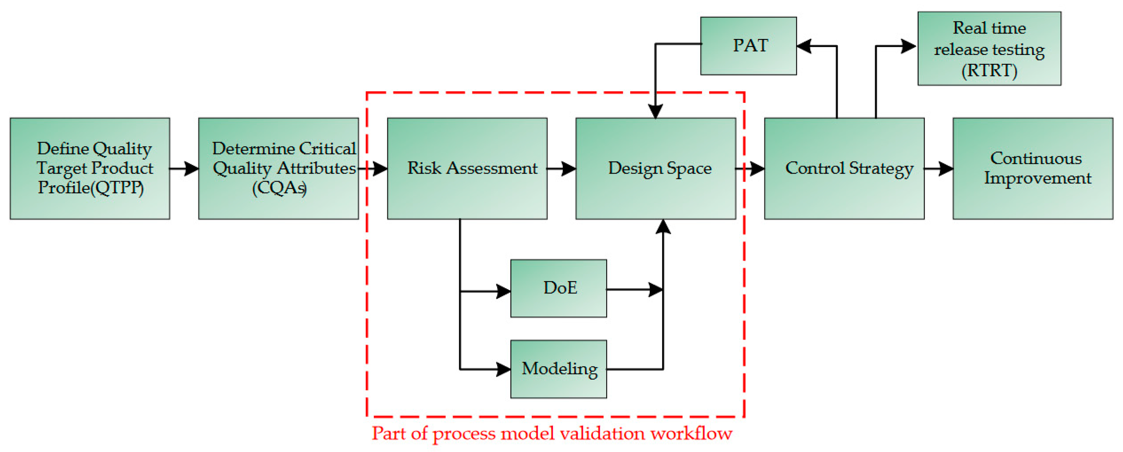
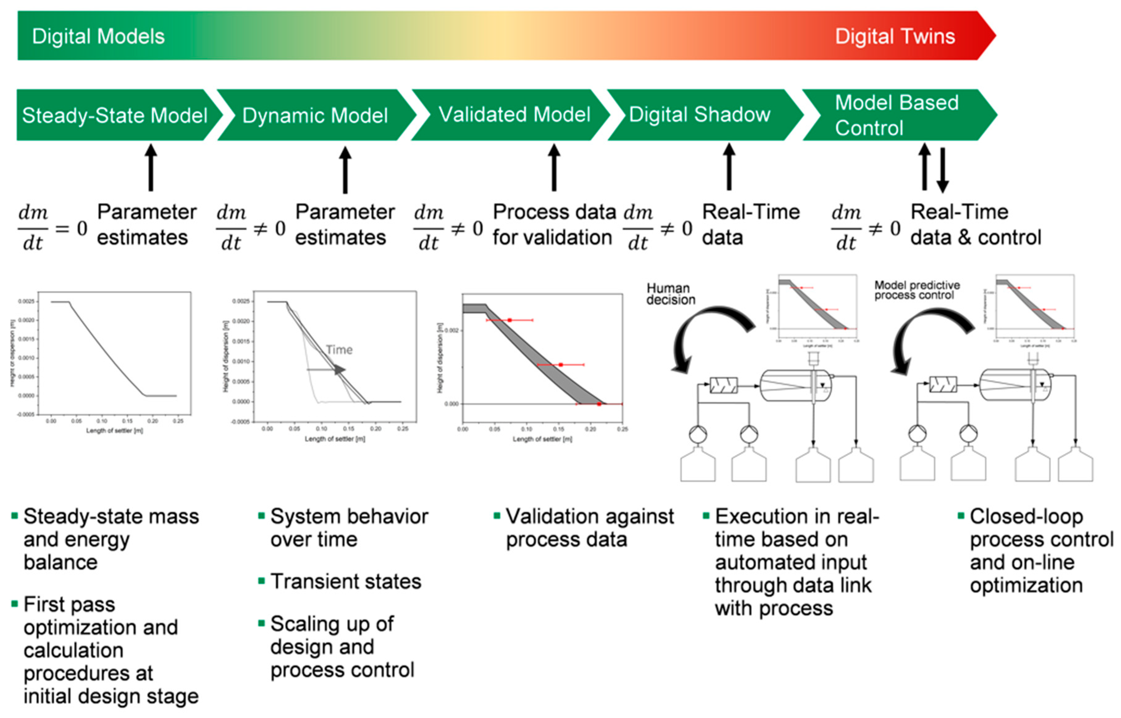
1.2. Quality by Design and Digital Twins
2. Review of Physiochemical Fundamentals for Scalable Digital Twin Modelling of Mixer–Settlers for Liquid–Liquid Extraction Process
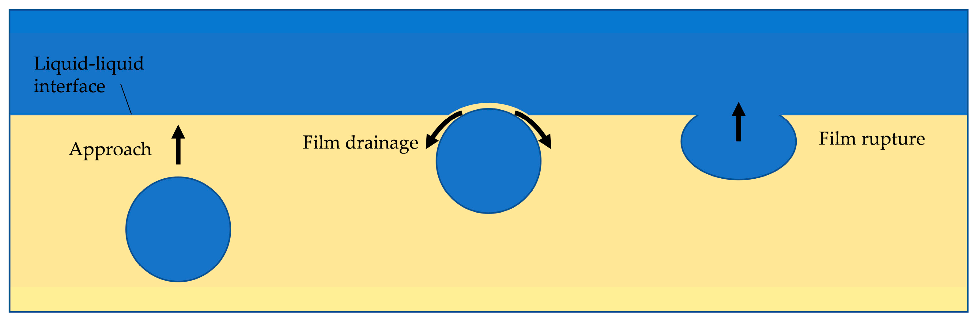
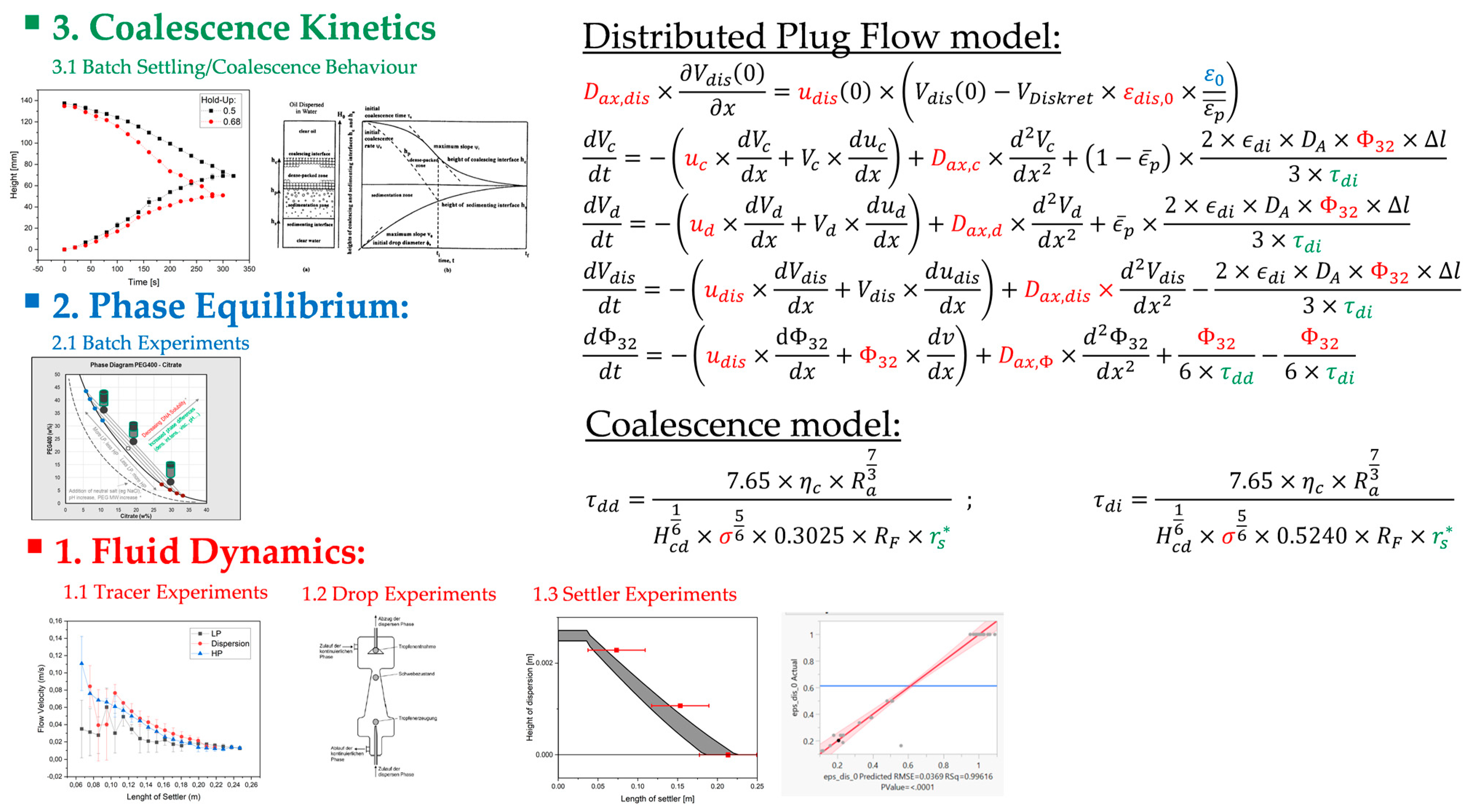
2.1. Fluid Dynamics
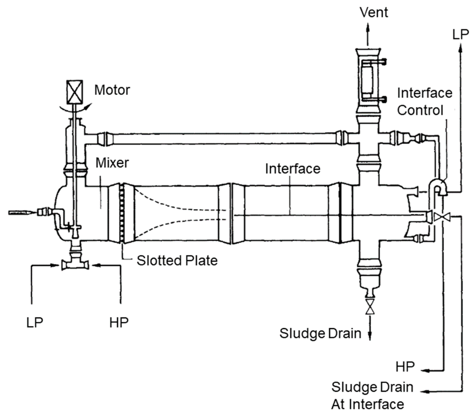
2.2. Continuous Settler Equipment
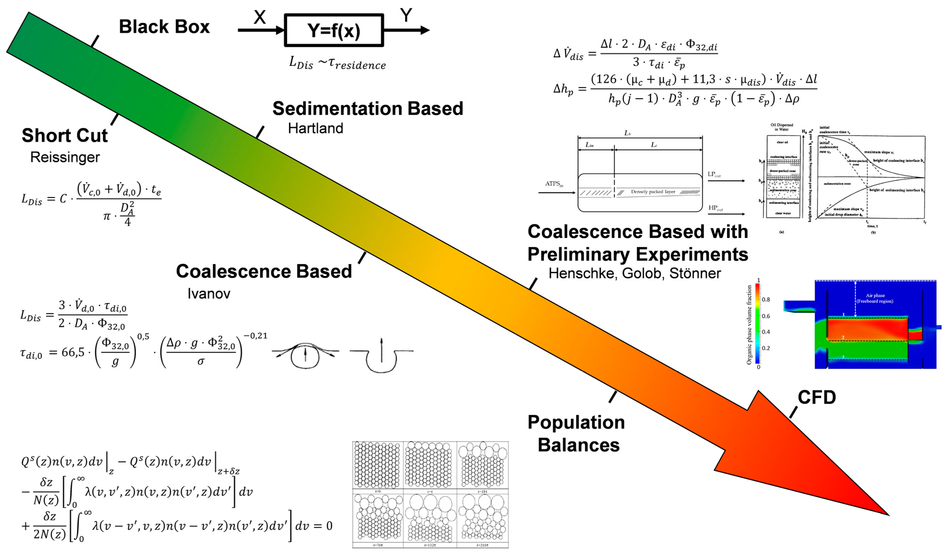
2.3. Settler Models
2.3.1. Modelling Depth
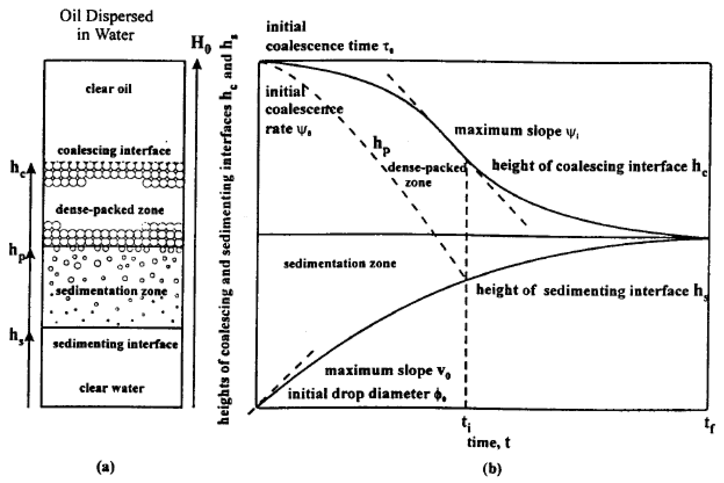
2.3.2. Henschke Model
- The vertical velocity in the film is neglected because the change in film thickness is very small compared to distance from the center of the film.
- The continuous phase is treated in the dispersion as an incompressible Newtonian fluid with constant viscosity.
- Gravity is negligible compared to the pressure due to the droplet packing.
- The film is considered to be two-dimensional.
- The spherical curvature of the film is neglected in the coalescence.
2.3.3. Computational Fluid Dynamics
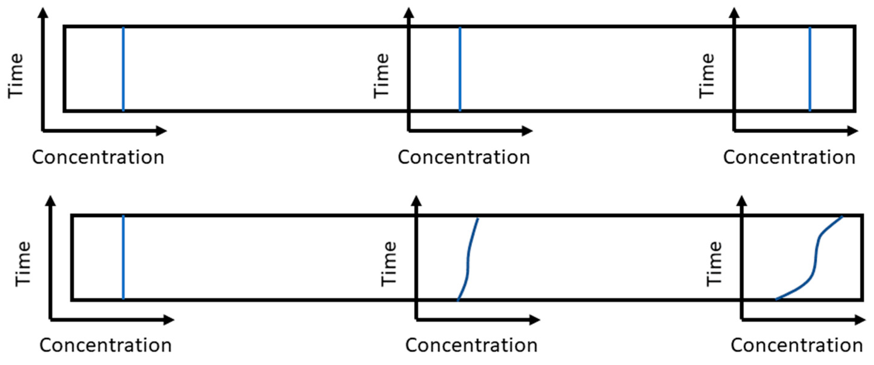
2.3.4. Distributed Plug Flow Model
- There is no concentration or velocity gradient in the radial direction.
- The model is one-dimensional.
- The convective transport is superimposed by a dispersive one.
- In the axial direction, material values, axial dispersion coefficient, and the geometric dimensions are assumed to be constant.
- A transient mass transport can be represented.
3. Material and Methods
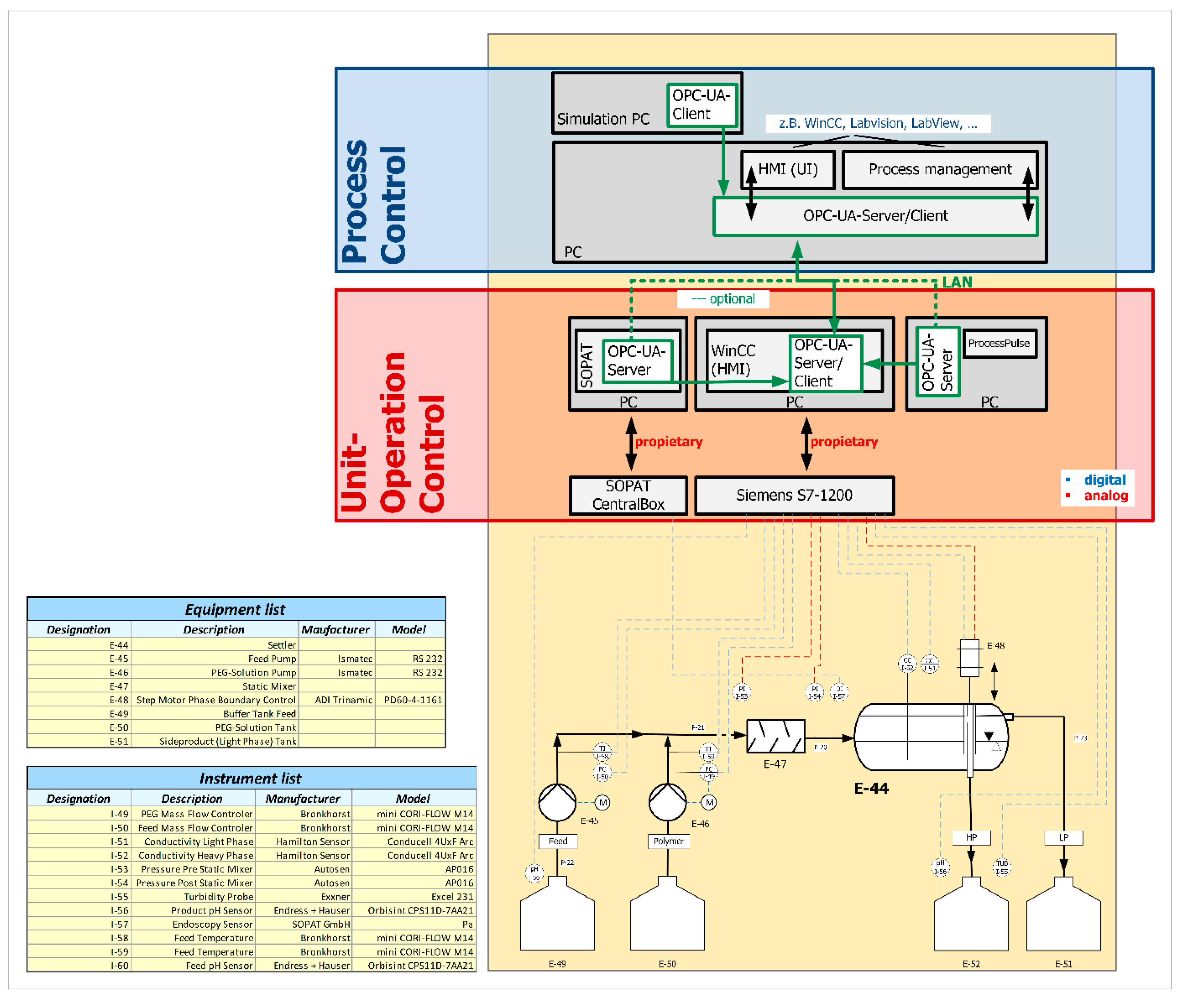
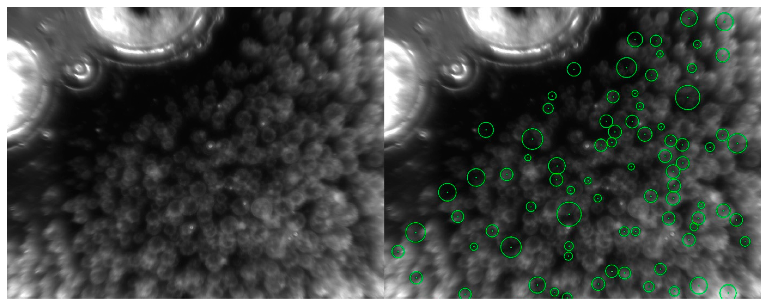
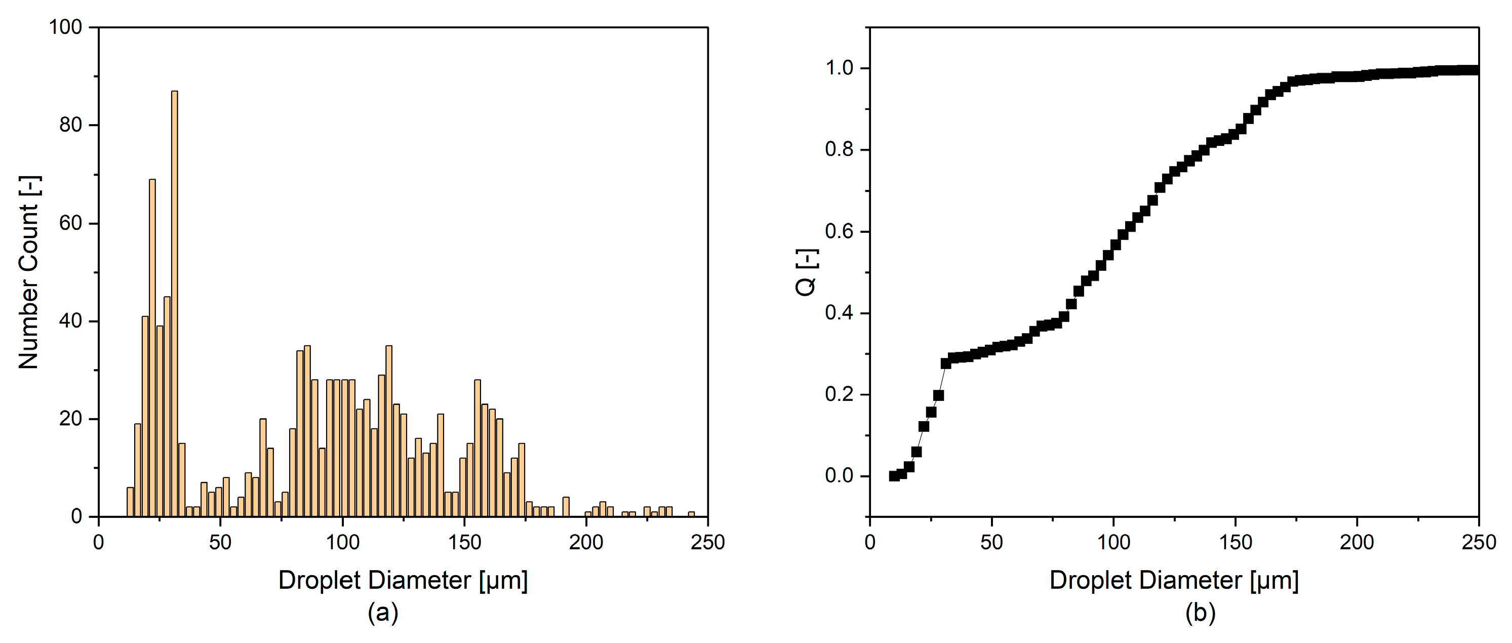
3.1. Process Analytical Technologies
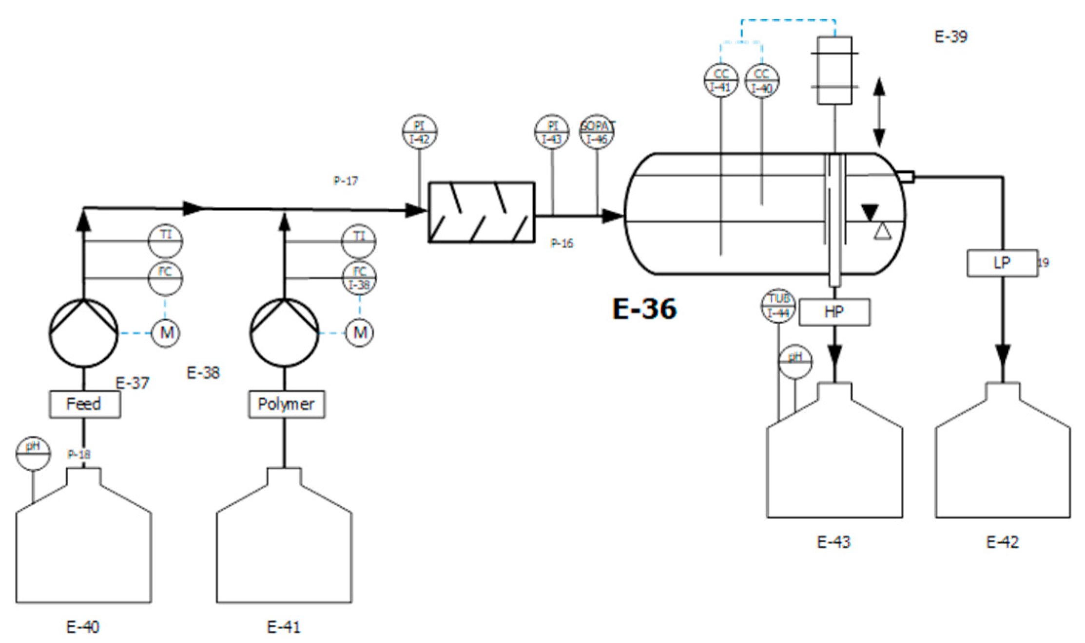
3.2. Experimental Setup
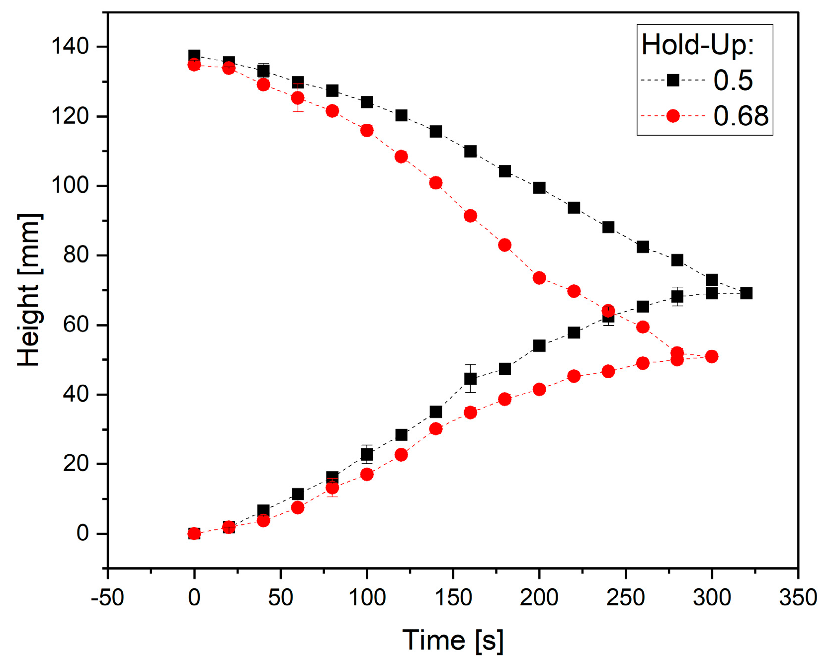
3.2.1. Batch Settling Experiments
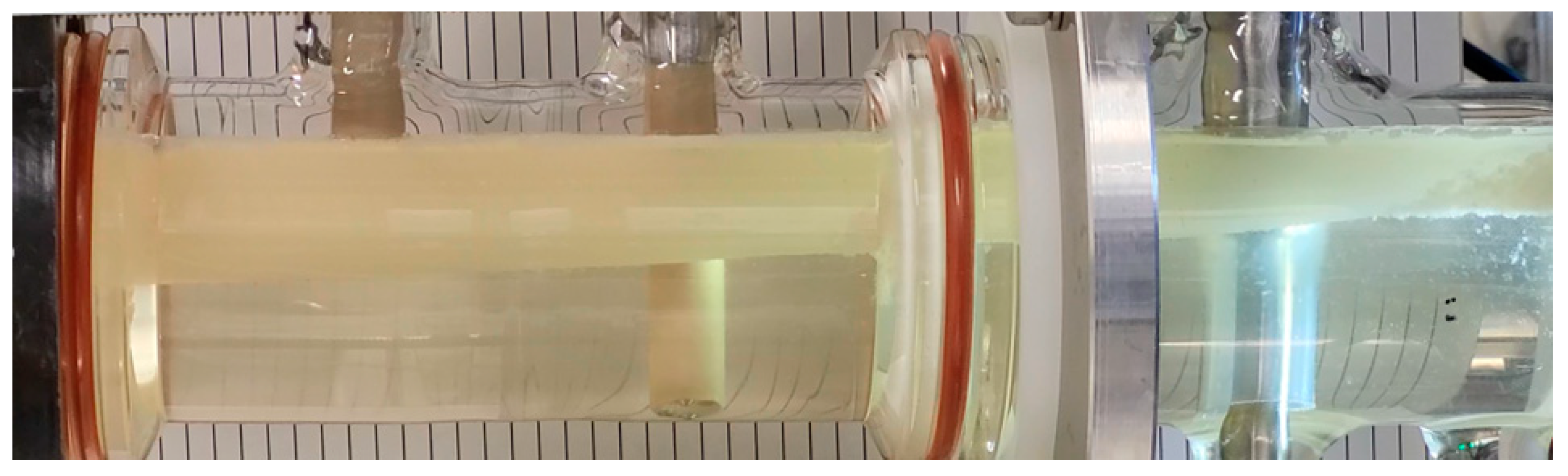
3.2.2. Continuous Horizontal Settler
3.2.3. Alkaline Lysis and ATPE
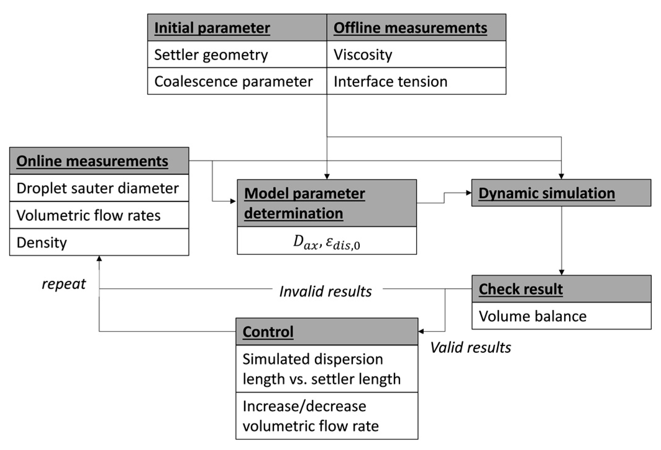
3.3. Continous Settler Process Model
4. Results
4.1. Implementation of the Digital Twin
4.2. Model Parameter Determination
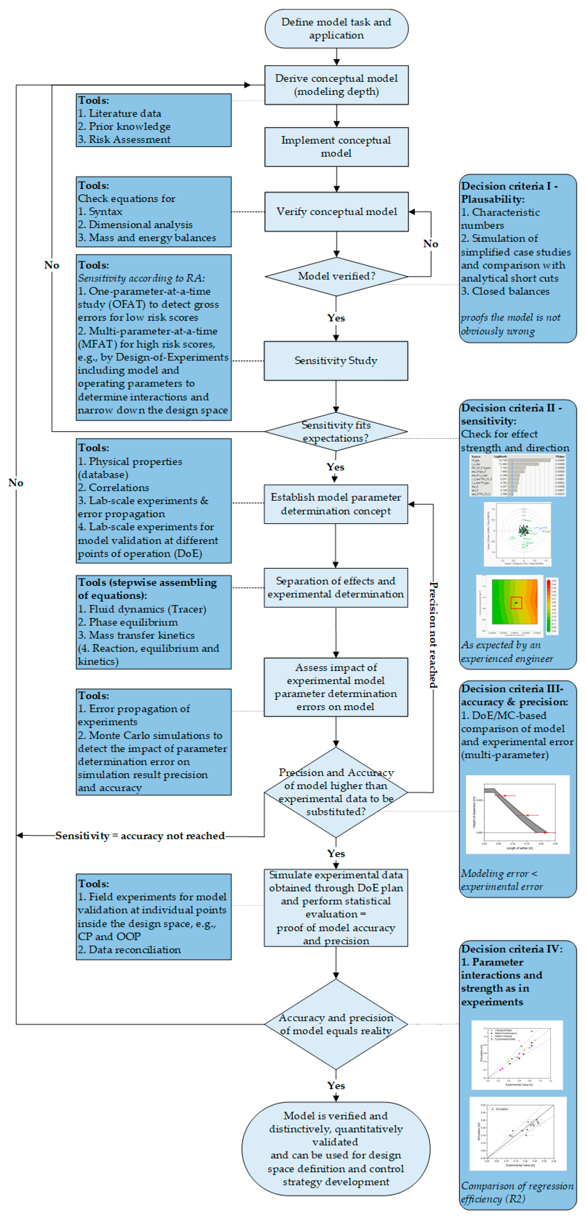
4.3. Validation of the Process Model
4.3.1. Plausibility
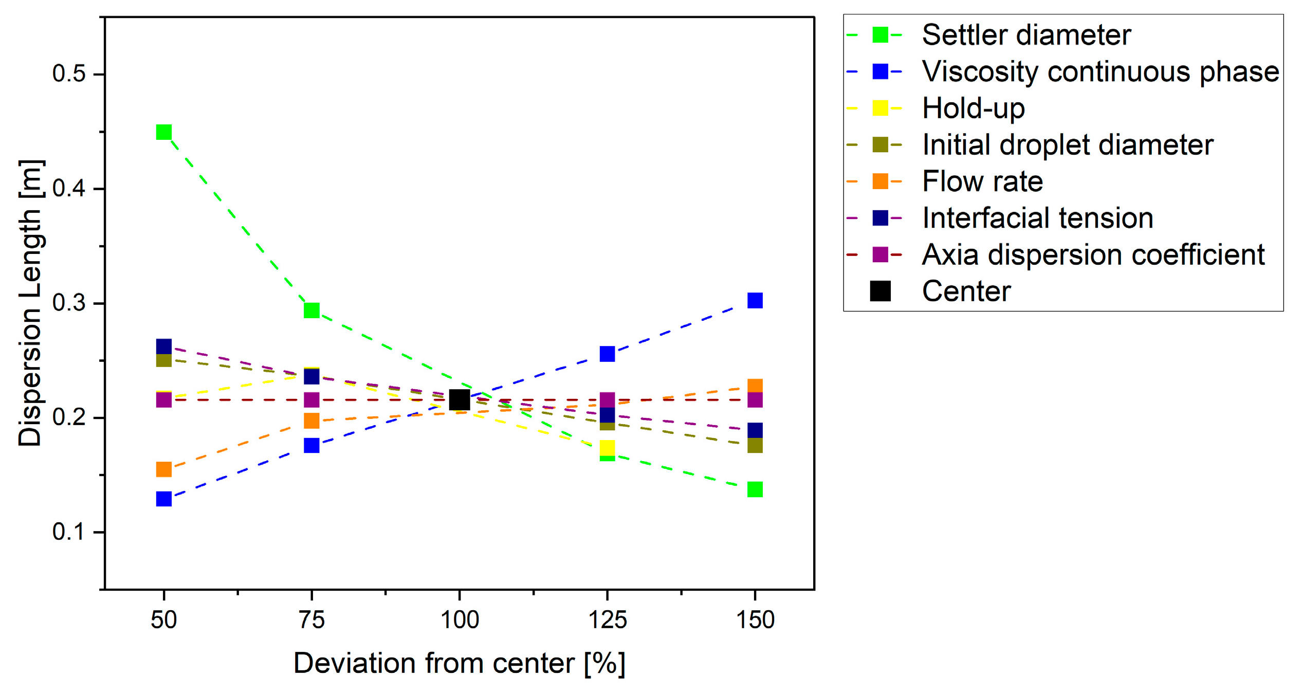
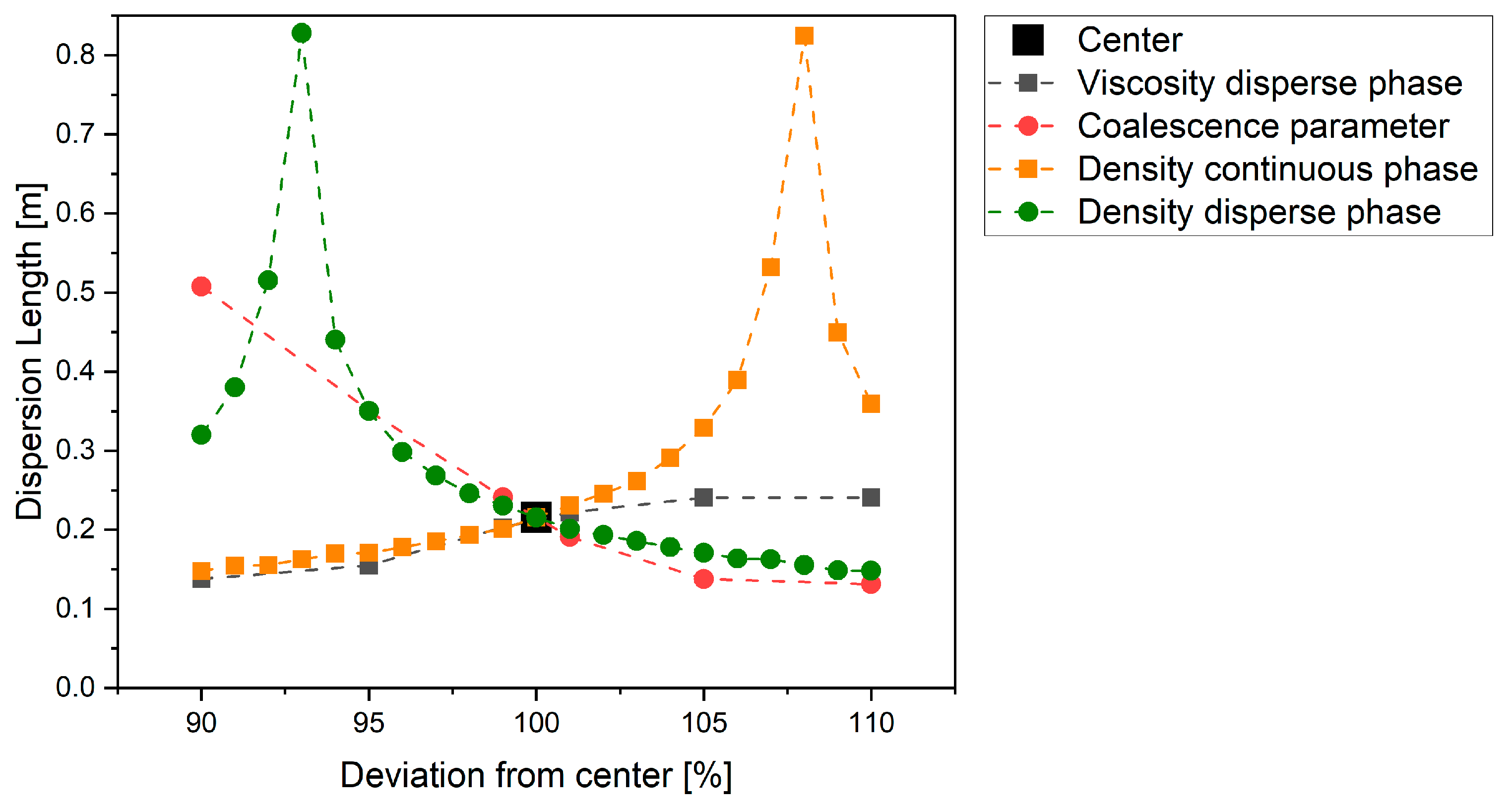
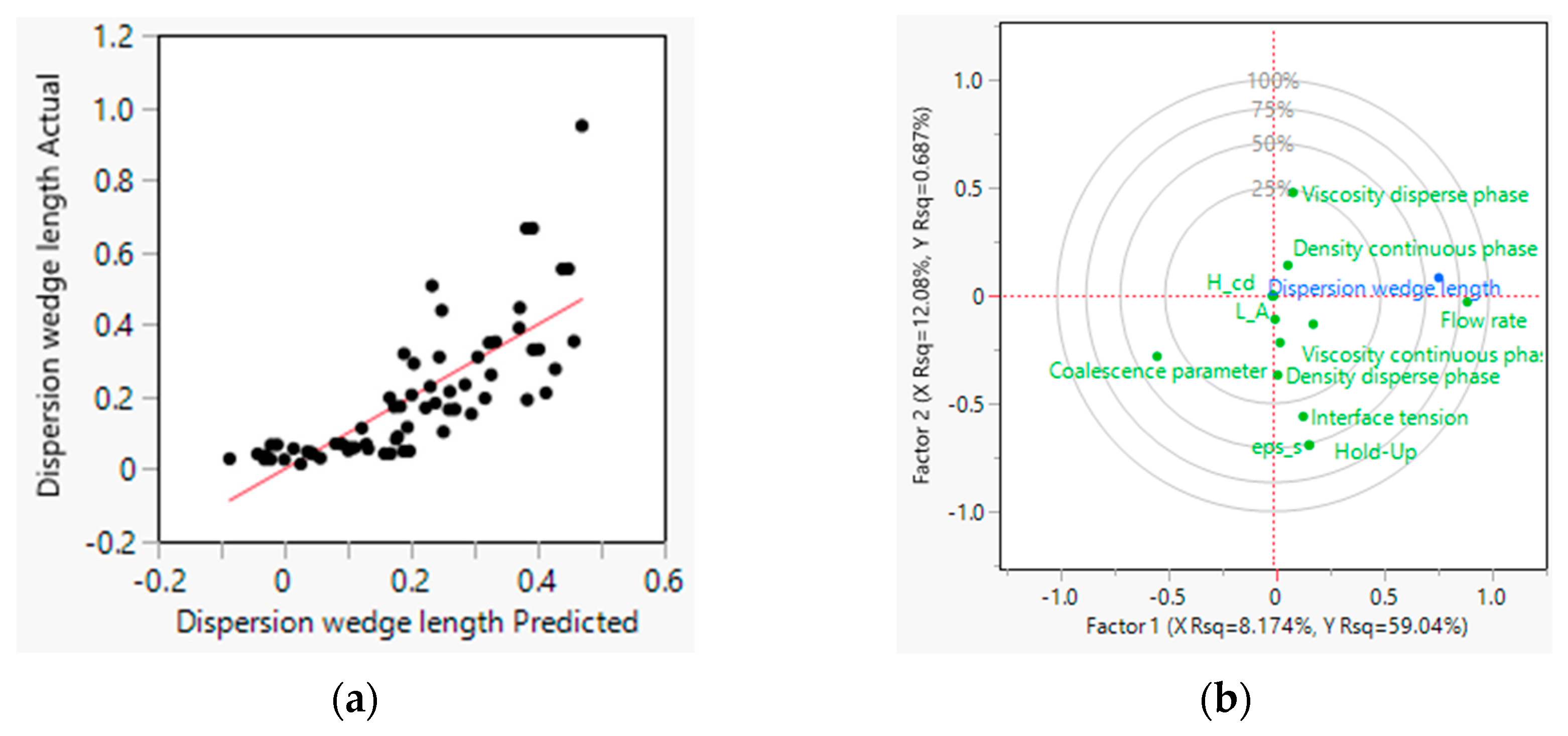
4.3.2. Sensitivity
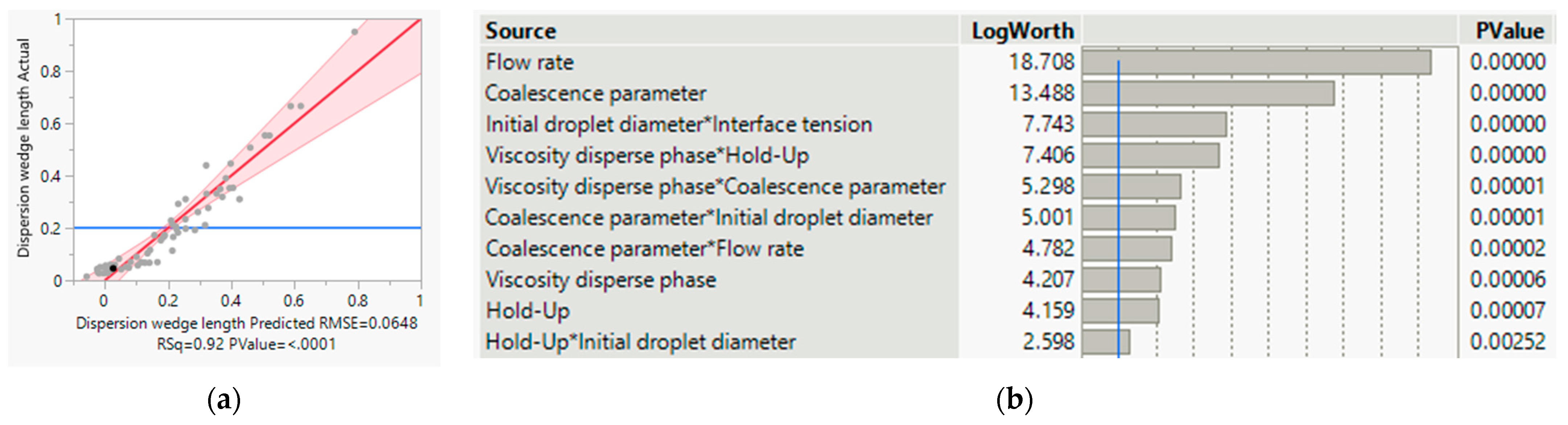
4.3.3. Precision
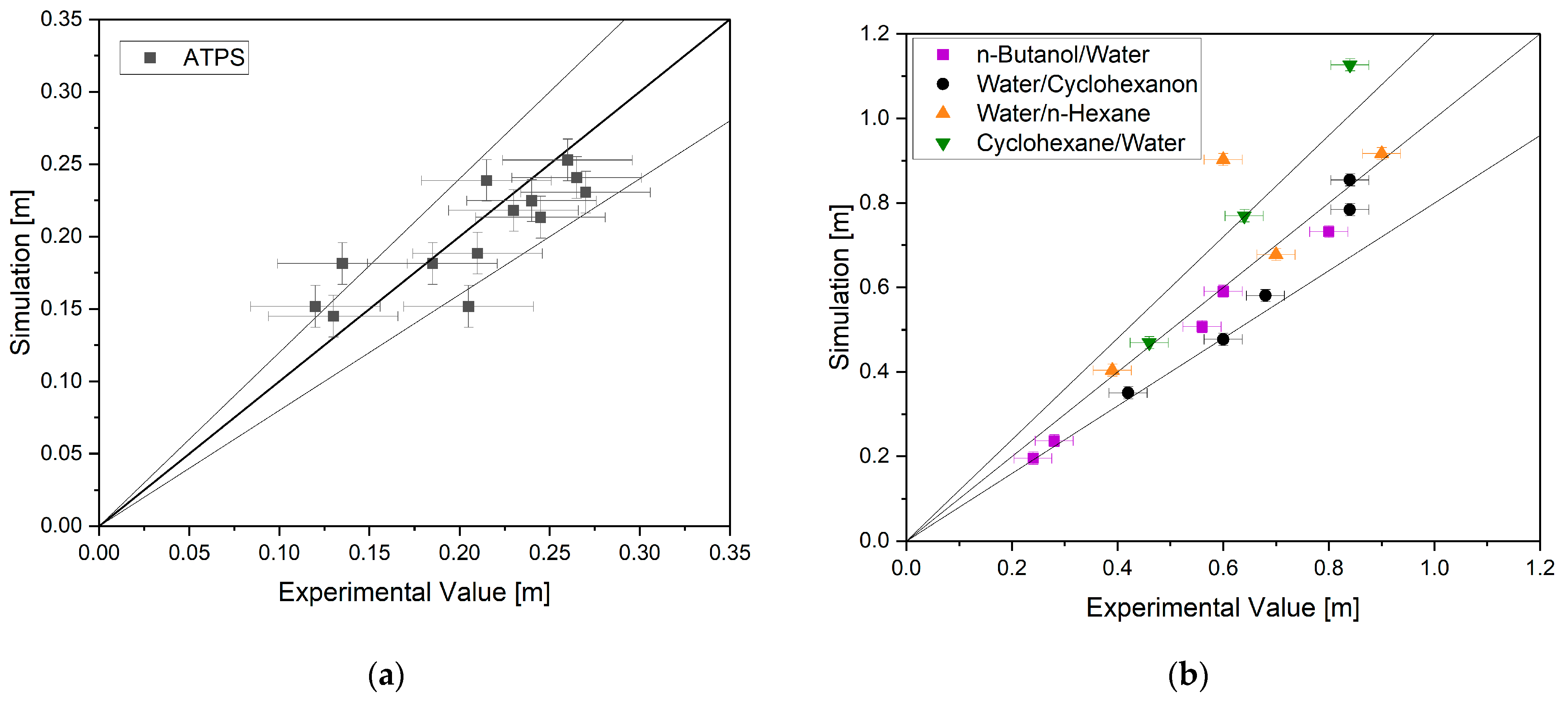
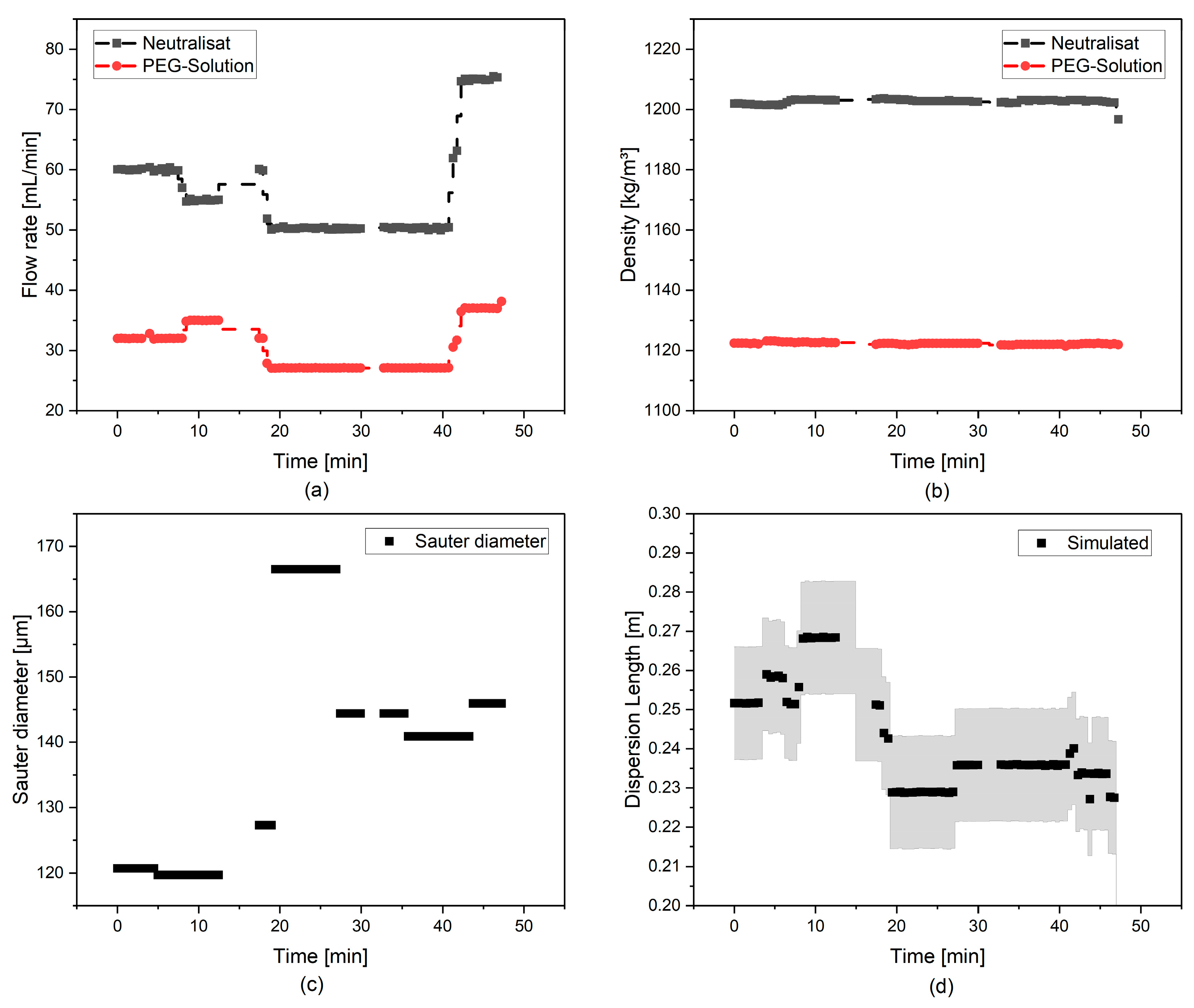
4.3.4. Accuracy and Validation
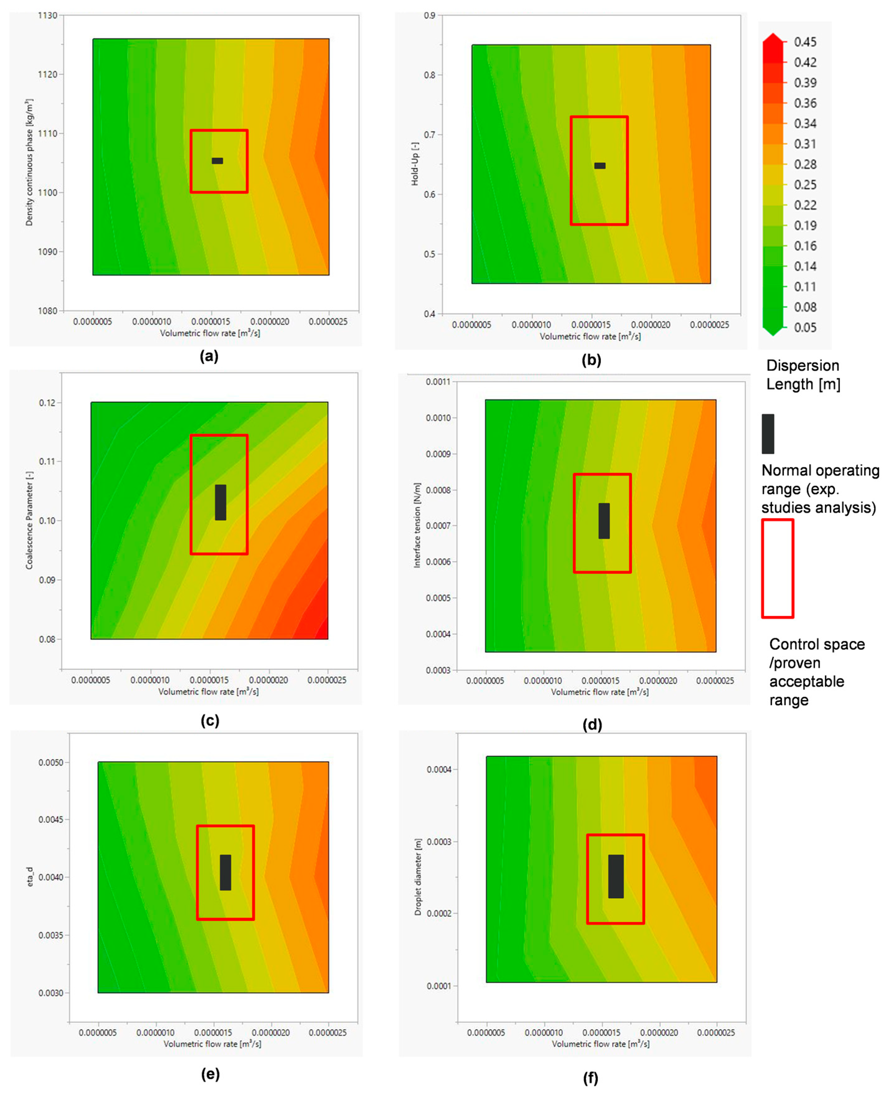
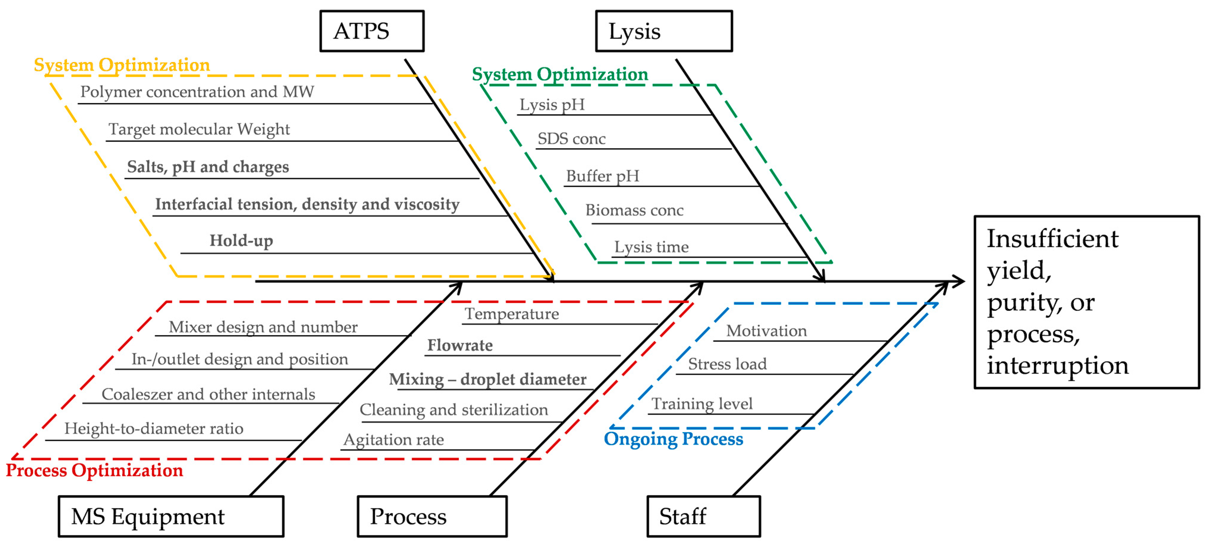
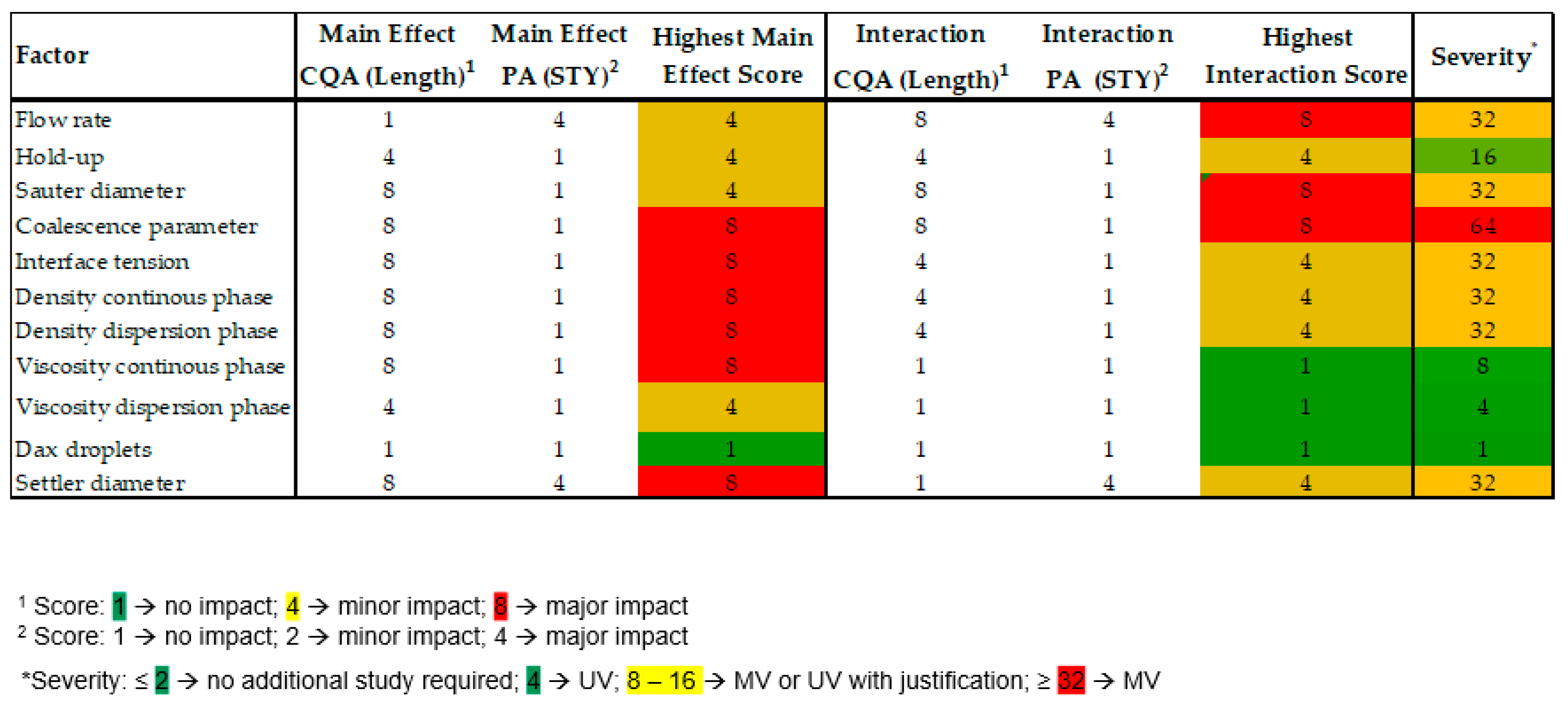
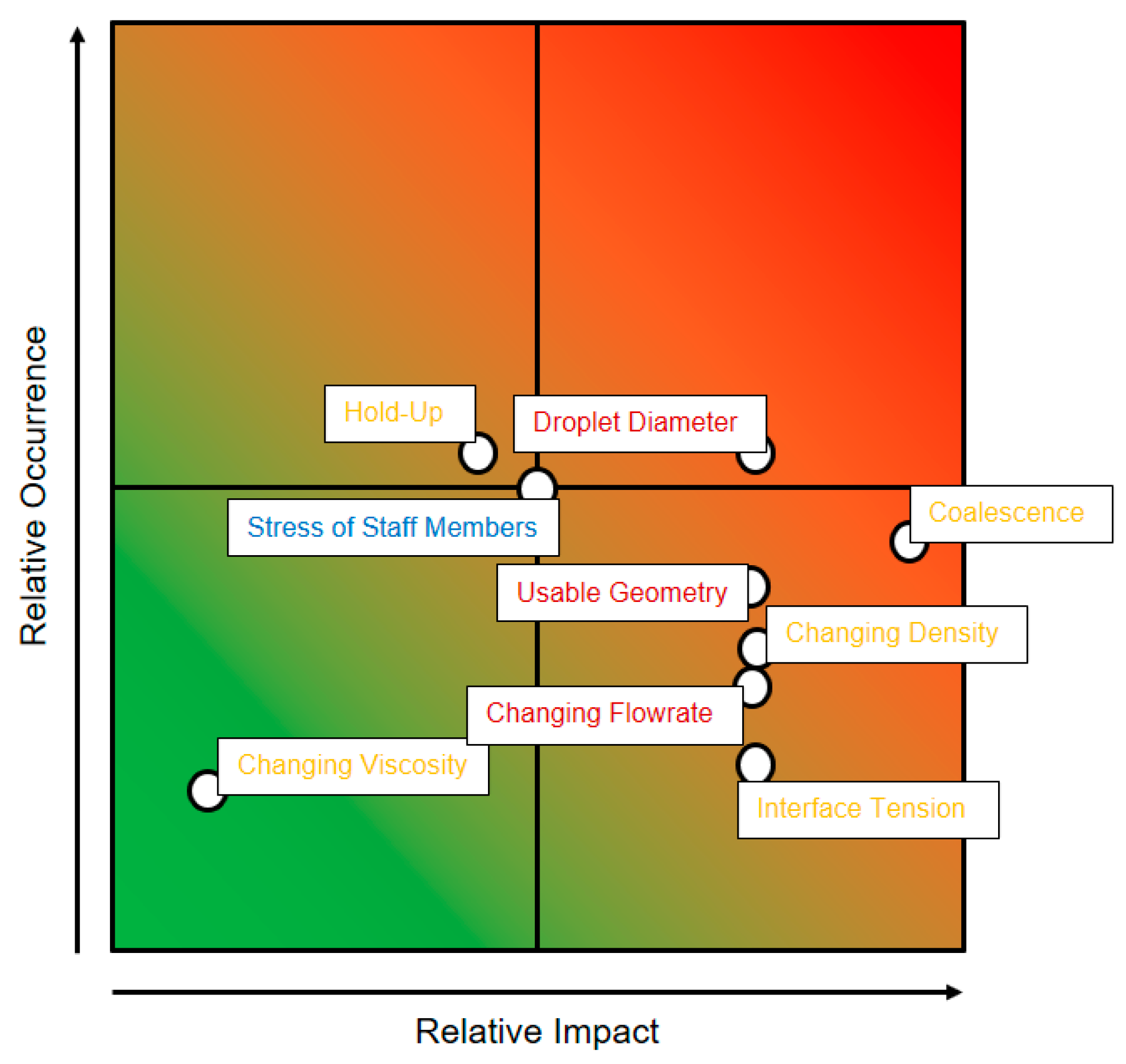
4.4. Risk Analysis
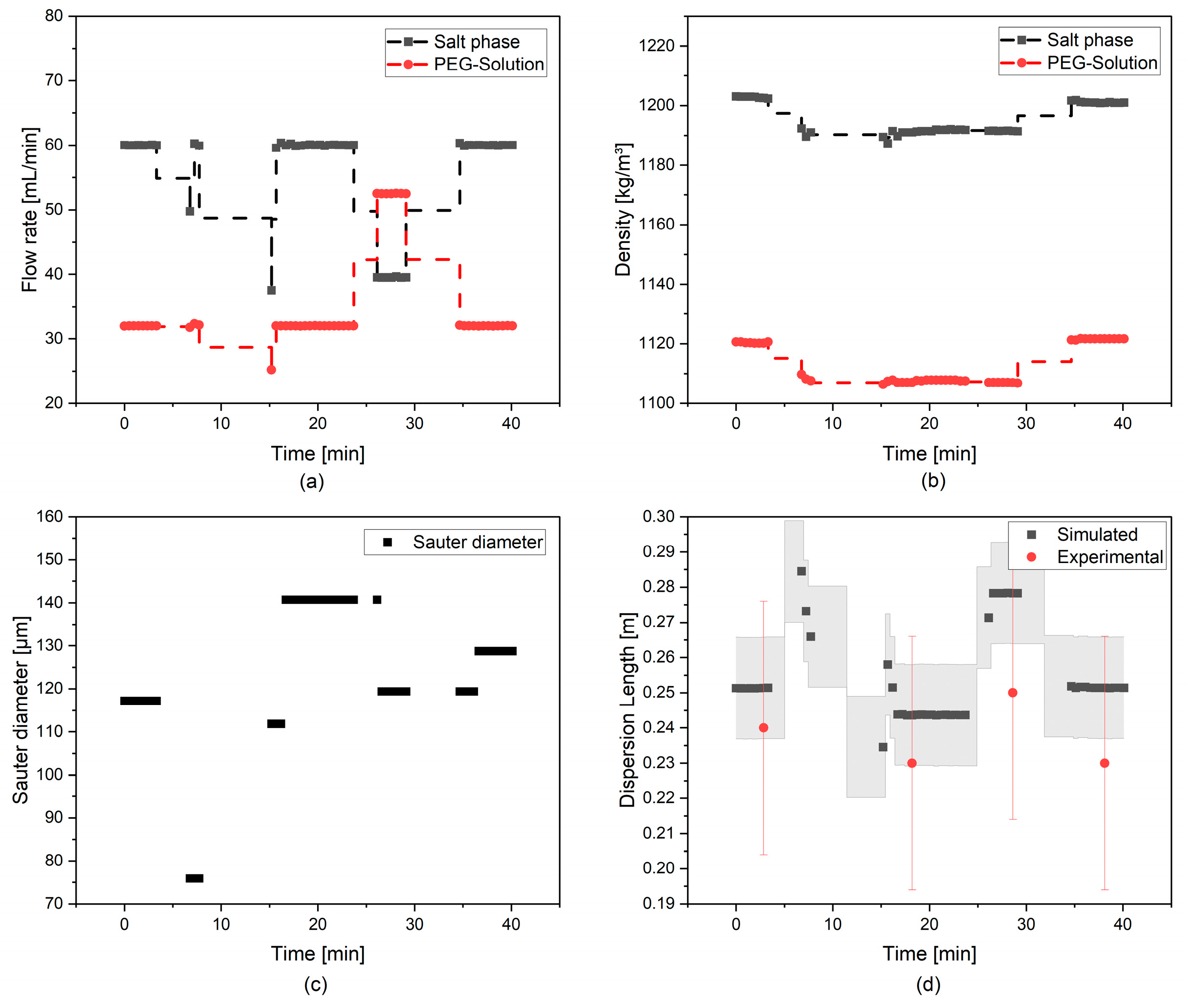
4.5. Experimental Feasibility by Autonomous Operation Study
5. Conclusions and Discussion
Author Contributions
Funding
Institutional Review Board Statement
Informed Consent Statement
Data Availability Statement
Acknowledgments
Conflicts of Interest
References
- Goedecke, R. Fluidverfahrenstechnik: Grundlagen, Methodik, Technik, Praxis; Wiley-VCH: Weinheim, Germany, 2006; ISBN 978-3-527-31198-9. [Google Scholar]
- Schmidt, A.; Strube, J. Application and Fundamentals of Liquid-Liquid Extraction Processes: Purification of Biologicals, Botanicals, and Strategic Metals. In Kirk-Othmer Encyclopedia of Chemical Technology; John Wiley & Sons, Inc.: Hoboken, NJ, USA, 2000; pp. 1–52. ISBN 9780471238966. [Google Scholar]
- Schmidt, A. Prozessintegration Mittels Validierter Digitaler Zwillinge von Flüssig-Flüssig-Extraktionsprozessen zur Gewinnung von Metallischen, Pflanzlichen und …; Shaker Verlag: Düren, Germany, 2021. [Google Scholar]
- dos Santos, N.V.; Carvalho Santos-Ebinuma, V.D.; Pessoa Junior, A.; Pereira, J.F.B. Liquid-liquid extraction of biopharmaceuticals from fermented broth: Trends and future prospects. J. Chem. Technol. Biotechnol. 2018, 93, 1845–1863. [Google Scholar] [CrossRef]
- Richter, M.C.; Rudolph, F.; Schmidt, A.; Strube, J. Verfahren zum reinigen und anreichern von proteinen, nukleinsäuren oder viren unter verwendung eines wässrigen zwei-phasen-systems. Patent WO2022157365A1, 28 June 2022. [Google Scholar]
- Helgers, H.; Hengelbrock, A.; Schmidt, A.; Vetter, F.L.; Juckers, A.; Strube, J. Digital Twins for scFv Production in Escherichia coli. Processes 2022, 10, 809. [Google Scholar] [CrossRef]
- Hengelbrock, A.; Helgers, H.; Schmidt, A.; Vetter, F.L.; Juckers, A.; Rosengarten, J.F.; Stitz, J.; Strube, J. Digital Twin for HIV-Gag VLP Production in HEK293 Cells. Processes 2022, 10, 866. [Google Scholar] [CrossRef]
- Schmidt, A.; Helgers, H.; Lohmann, L.J.; Vetter, F.; Juckers, A.; Mouellef, M.; Zobel-Roos, S.; Strube, J. Process analytical technology as key-enabler for digital twins in continuous biomanufacturing. J. Chem. Technol. Biotechnol. 2022, 97, 2336–2346. [Google Scholar] [CrossRef]
- Helgers, H.; Hengelbrock, A.; Schmidt, A.; Strube, J. Digital Twins for Continuous mRNA Production. Processes 2021, 9, 1967. [Google Scholar] [CrossRef]
- Kritzinger, W.; Karner, M.; Traar, G.; Henjes, J.; Sihn, W. Digital Twin in manufacturing: A categorical literature review and classification. IFAC-PapersOnLine 2018, 51, 1016–1022. [Google Scholar] [CrossRef]
- Sixt, M. Methoden zur Systematischen Gesamtprozessentwicklung und Prozessintensivierung von Extraktions-und Trennprozessen zur Gewinnung Pflanzlicher Wertkomponenten; Shaker Verlag: Düren, Germany, 2018. [Google Scholar]
- Pharmaceutical Development Q8(R2): International Conference on Harmonisation of Technical Requirements for Registration of Pharmaceuticals for Human Use; ICH: Geneva, Switzerland, 2009.
- Uhlenbrock, L.; Sixt, M.; Strube, J. Quality-by-Design (QbD) process evaluation for phytopharmaceuticals on the example of 10-deacetylbaccatin III from yew. Resou.-Eff. Technol. 2017, 3, 137–143. [Google Scholar] [CrossRef]
- Henschke, M. Dimensionierung Liegender Flüssig-Flüssig-Abscheider Anhand Diskontinuierlicher Absetzversuche; Zugl.: Aachen, Techn. Hochsch., Diss., 1994, Als Ms. gedr; VDI-Verl.: Düsseldorf, Germany, 1995; ISBN 3-18-337903-1. [Google Scholar]
- Narasingam, A.; Kwon, J.S.-I. Development of local dynamic mode decomposition with control: Application to model predictive control of hydraulic fracturing. Comput. Chem. Eng. 2017, 106, 501–511. [Google Scholar] [CrossRef]
- Shi, D.; Mhaskar, P.; El-Farra, N.H.; Christofides, P.D. Predictive control of crystal size distribution in protein crystallization. Nanotechnology 2005, 16, S562–S574. [Google Scholar] [CrossRef] [PubMed]
- Henschke, M.; Pfennig, A. Simulation of Packed Extraction Columns with the REDROP Model; Czech Society of Chemical Engineering: Praha, Tsjechië, 1996; ISBN 80-02-01106-6 1130. [Google Scholar]
- Ayesterán, J.; Kopriwa, N.; Buchbender, F.; Kalem, M.; Pfennig, A. ReDrop–A Simulation Tool for the Design of Extraction Columns Based on Single-Drop Experiments. Chem. Eng. Technol. 2015, 38, 1894–1900. [Google Scholar] [CrossRef]
- Hlawitschka, M.W.; Schäfer, J.; Hummel, M.; Garth, C.; Bart, H.-J. Populationsbilanzmodellierung mit einem Mehrphasen-CFD-Code und vergleichende Visualisierung. Chem. Ingenieur Tech. 2016, 88, 1480–1491. [Google Scholar] [CrossRef]
- Hlawitschka, M.W.; Jaradat, M.; Chen, F.; Attarakih, M.M.; Kuhnert, J.; Bart, H.-J. A CFD-Population Balance Model for the Simulation of Kühni Extraction Column. In 21st European Symposium on Computer Aided Process Engineering; Elsevier: Amsterdam, The Netherlands, 2011; pp. 66–70. ISBN 9780444538956. [Google Scholar]
- Drumm, C.; Attarakih, M.; Hlawitschka, M.W.; Bart, H.-J. One-Group Reduced Population Balance Model for CFD Simulation of a Pilot-Plant Extraction Column. Ind. Eng. Chem. Res. 2010, 49, 3442–3451. [Google Scholar] [CrossRef]
- Mühlbauer, A.; Hlawitschka, M.W.; Bart, H.-J. Models for the Numerical Simulation of Bubble Columns: A Review. Chem. Ingenieur Tech. 2019, 91, 1747–1765. [Google Scholar] [CrossRef]
- Casamatta, G.; Vogelpohl, A. Modellierung der Fluiddynamik und des Stoffübergangs in Extraktionskolonnen. Chem. Ingenieur Tech. 1984, 56, 230–231. [Google Scholar] [CrossRef]
- Lohrengel, B. Thermische Trennverfahren: Trennung von Gas-, Dampf-und Flüssigkeitsgemischen, 3rd ed.; De Gruyter Oldenbourg: Berlin, Germany, 2017; ISBN 978-3-11-047321-6. [Google Scholar]
- Rommel, W.; Meon, W.; Blass, E. Hydrodynamic Modeling of Droplet Coalescence at Liquid-Liquid Interfaces. Sep. Sci. Technol. 1992, 27, 129–159. [Google Scholar] [CrossRef]
- Jeelani, S.A.K.; Hartland, S. Effect of Dispersion Properties on the Separation of Batch Liquid−Liquid Dispersions. Ind. Eng. Chem. Res. 1998, 37, 547–554. [Google Scholar] [CrossRef]
- Mersmann, A.; Stichlmair, J.; Kind, M. Thermische Verfahrenstechnik: Grundlagen und Methoden; 2., wesentlich erweiterte and aktualisierte Auflage; Springer: Berlin, Germany, 2005; ISBN 3540280529. [Google Scholar]
- Sattler, K. Thermische Trennverfahren: Grundlagen, Auslegung, Apparate; 3., überarb. u. erw. Aufl., [Nachdr.]; Wiley-VCH: Weinheim, Germany, 2007; ISBN 9783527302437. [Google Scholar]
- Brandt, H.W.; Reissinger, K.-H.; Schröter, J. Moderne Flüssig/Flüssig-Extraktoren-Übersicht und Auswahlkriterien. Chem. Ingenieur Tech. 1978, 50, 345–354. [Google Scholar] [CrossRef]
- Schmidt, A.; Richter, M.; Rudolph, F.; Strube, J. Integration of Aqueous Two-Phase Extraction as Cell Harvest and Capture Operation in the Manufacturing Process of Monoclonal Antibodies. Antibodies 2017, 6, 21. [Google Scholar] [CrossRef]
- Hui, Y.H.; Bruinsma, B. (Eds.) Food Plant Sanitation; Dekker: New York, NY, USA, 2003; ISBN 0824707931. [Google Scholar]
- Strube, J.; Schulte, M. Thermische Trennverfahren als Schlüsseltechnologie in den Life Sciences. Chem. Ingenieur Tech. 2003, 75, 1071–1072. [Google Scholar] [CrossRef]
- Frising, T.; Noïk, C.; Dalmazzone, C. The Liquid/Liquid Sedimentation Process: From Droplet Coalescence to Technologically Enhanced Water/Oil Emulsion Gravity Separators: A Review. J. Dispers. Sci. Technol. 2006, 27, 1035–1057. [Google Scholar] [CrossRef]
- Ruiz, M.C.; Padilla, R. Separation of liquid-liquid dispersions in a deep-layer gravity settler: Part II. Mathematical modeling of the settler. Hydrometallurgy 1996, 42, 281–291. [Google Scholar] [CrossRef]
- Reissinger, K.-H.; Schröter, J.; Bäcker, W. Möglichkeiten und Probleme bei der Auslegung von Extraktoren. Chem. Ingenieur Tech. 1981, 53, 607–614. [Google Scholar] [CrossRef]
- Hartland, S. Koaleszenz in dichtgepackten Gas/Flüssig-und Flüssig/Flüssig-Dispersionen. Ber. Der Bunsenges. Für Physikalische Chem. 1981, 85, 851–863. [Google Scholar] [CrossRef]
- Panda, S.K.; Buwa, V.V. Effects of Geometry and Internals of a Continuous Gravity Settler on Liquid–Liquid Separation. Ind. Eng. Chem. Res. 2017, 56, 13929–13944. [Google Scholar] [CrossRef]
- Stönner, H.M. Proceedings of the Mathematisches Modell für den Flüssig-Flüssig-Abscheide-Vorgang (am Beispiel der dichtgepackten Dispersion): Vortrag Anlässlich der Sitzung des Extraktionsgremiums, Frankfurt/Main, Duitsland, 20 March 1981.
- Yaron, I.; Gal-Or, B. On viscous flow and effective viscosity of concentrated suspensions and emulsions. Rheol. Acta 1972, 11, 241–252. [Google Scholar] [CrossRef]
- Ferziger, J.H. Numerische Strömungsmechanik; Springer: Berlin/Heidelberg, Germany, 2008; ISBN 978-3-540-68228-8. [Google Scholar]
- Singh, K.K.; Sarkar, S.; Sen, N.; Mukhopadhyay, S.; Shenoy, K.T. Computational fluid dynamics modelling of solvent extraction equipment: A review. BARC Newslett. 2021, 379, 45–55. [Google Scholar]
- Panda, S.K.; Singh, K.K.; Shenoy, K.T.; Buwa, V.V. Numerical simulations of liquid-liquid flow in a continuous gravity settler using OpenFOAM and experimental verification. Chem. Eng. J. 2017, 310, 120–133. [Google Scholar] [CrossRef]
- Shabani, M.O.; Mazahery, A.; Alizadeh, M.; Tofigh, A.A.; Rahimipour, M.R.; Razavi, M.; Kolahi, A. Computational fluid dynamics (CFD) simulation of effect of baffles on separation in mixer settler. Int. J. Min. Sci. Technol 2012, 22, 703–706. [Google Scholar] [CrossRef]
- Schmidt, A.; Montenegro, V.; Wehinger, G.D. Transient CFD Modeling of Matte Settling Behavior and Coalescence in an Industrial Copper Flash Smelting Furnace Settler. Metall. Mater. Trans. B 2021, 52, 405–413. [Google Scholar] [CrossRef]
- Shabani, M.; Mazahery, A. Computational Fluid Dynamics (CFD) Simulation of Liquid-Liquid Mixing in Mixer Settler. Arch. Metall. Mat. 2012, 57, 173–178. [Google Scholar] [CrossRef]
- Kankaanpää, T. CFD Procedure for Studying Dispersion Flows and Design Optimization of the Solvent Extraction Settler; Helsinki University of Technology, Laboratory of Materials Processing and Powder Metallurgy: Espoo, Finland, 2007; ISBN 1795-0074. [Google Scholar]
- Hlawitschka, M. ERNA—Effiziente Tropfenabscheidung in Flüssig-Flüssig-Systemen an Gestricken: Schlussbericht; 2021. Schlussbericht zu IGF-Vorhaben 19743 N/1: Berichtszeitraum: 01.10.2017–30.06.2020. Available online: https://books.google.ro/books/about/ERNA_Effiziente_Tropfenabscheidung_in_Fl.html?id=3CbyzgEACAAJ&redir_esc=y (accessed on 6 January 2023).
- Danckwerts, P.V. Continuous flow systems. Chem. Eng. Sci. 1953, 2, 1–13. [Google Scholar] [CrossRef]
- Güttel, R.; Turek, T. Chemische Reaktionstechnik; 1. Aufl. 2021; Springer: Berlin/Heidelberg, Germany, 2021; ISBN 9783662631508. [Google Scholar]
- Emmerich, J.; Tang, Q.; Wang, Y.; Neubauer, P.; Junne, S.; Maaß, S. Optical inline analysis and monitoring of particle size and shape distributions for multiple applications: Scientific and industrial relevance. Chin. J. Chem. Eng. 2019, 27, 257–277. [Google Scholar] [CrossRef]
- Henschke, M. Determination of a coalescence parameter from batch-settling experiments. Chem. Eng. J. 2002, 85, 369–378. [Google Scholar] [CrossRef]
- Urthaler, J.; Buchinger, W.; Necina, R. Improved downstream process for the production of plasmid DNA for gene therapy. Acta Biochim. Pol. 2005, 52, 703–711. [Google Scholar] [CrossRef] [PubMed]
- Levenspiel. Chemical Reaction Engineering; John Wiley and Sons Inc: Hoboken, NJ, USA, 1999. [Google Scholar]
- Trivedi, R.N.; Vasudeva, K. Axial dispersion in laminar flow in helical coils. Chem. Eng. Sci. 1975, 30, 317–325. [Google Scholar] [CrossRef]
- Sixt, M.; Uhlenbrock, L.; Strube, J. Toward a Distinct and Quantitative Validation Method for Predictive Process Modelling—On the Example of Solid-Liquid Extraction Processes of Complex Plant Extracts. Processes 2018, 6, 66. [Google Scholar] [CrossRef]
- Reynolds, O. XXIX. An experimental investigation of the circumstances which determine whether the motion of water shall be direct or sinuous, and of the law of resistance in parallel channels. Phil. Trans. R. Soc. 1883, 174, 935–982. [Google Scholar] [CrossRef]
- Dessimoz, A.-L.; Cavin, L.; Renken, A.; Kiwi-Minsker, L. Liquid–liquid two-phase flow patterns and mass transfer characteristics in rectangular glass microreactors. Chem. Eng. Sci. 2008, 63, 4035–4044. [Google Scholar] [CrossRef]
- Kralj, S.; Eeuwema, W.; Eckhardt, T.H.; Dijkhuizen, L. Role of asparagine 1134 in glucosidic bond and transglycosylation specificity of reuteransucrase from Lactobacillus reuteri 121. FEBS J. 2006, 273, 3735–3742. [Google Scholar] [CrossRef]
- Mewes, D.; Pilhofer, T. Vorausberechnung der fluiddynamischen Eigenschaften von Siebbodenextraktionskolonnen ohne Pulsation. Chem. Ingenieur Tech. 1978, 50, 203–211. [Google Scholar] [CrossRef]


| Characteristic Number | Region | Lowest Value | Highest Value |
|---|---|---|---|
| Reynolds number | Inlet | 3.26 × 10² | 7.99 × 10³ |
| Settler | 3.03 × 10⁻³ | 6.18 × 10⁻¹ | |
| Weber number | Inlet | 1.25 × 10⁻⁴ | 4.40 × 10⁻² |
| Settler | 1.61 × 10⁻⁴ | 9.28 × 10⁻² | |
| Bond number | Inlet | 1.03 × 10⁻² | 8.93 × 10⁻¹ |
| Settler | 1.48 × 10⁻² | 3.50 × 100 | |
| Archimedes number | Inlet | 7.34 × 101 | 2.46 × 10³ |
| Settler | 1.17 × 10² | 7.26 × 10³ |
| Parameter | Unit | Lower Boundary | Upper Boundary |
|---|---|---|---|
| Flow rate | [m³/s] | ||
| Density continuous phase | [kg/m³] | 1086 | 1126 |
| Density disperse phase | [kg/m³] | 1172 | 1212 |
| Viscosity continuous phase | [Pa s] | 0.007 | 0.009 |
| Viscosity disperse phase | [Pa s] | 0.003 | 0.005 |
| Initial droplet diameter | [µm] | 418 | 1045 |
| Interface tension | [N/m] | ||
| Hold-Up | [-] | 0.40 | 0.85 |
| Coalescence parameter | [-] | 0.08 | 0.12 |
Disclaimer/Publisher’s Note: The statements, opinions and data contained in all publications are solely those of the individual author(s) and contributor(s) and not of MDPI and/or the editor(s). MDPI and/or the editor(s) disclaim responsibility for any injury to people or property resulting from any ideas, methods, instructions or products referred to in the content. |
© 2023 by the authors. Licensee MDPI, Basel, Switzerland. This article is an open access article distributed under the terms and conditions of the Creative Commons Attribution (CC BY) license (https://creativecommons.org/licenses/by/4.0/).
Share and Cite
Uhl, A.; Schmidt, A.; Hlawitschka, M.W.; Strube, J. Autonomous Liquid–Liquid Extraction Operation in Biologics Manufacturing with Aid of a Digital Twin including Process Analytical Technology. Processes 2023, 11, 553. https://doi.org/10.3390/pr11020553
Uhl A, Schmidt A, Hlawitschka MW, Strube J. Autonomous Liquid–Liquid Extraction Operation in Biologics Manufacturing with Aid of a Digital Twin including Process Analytical Technology. Processes. 2023; 11(2):553. https://doi.org/10.3390/pr11020553
Chicago/Turabian StyleUhl, Alexander, Axel Schmidt, Mark W. Hlawitschka, and Jochen Strube. 2023. "Autonomous Liquid–Liquid Extraction Operation in Biologics Manufacturing with Aid of a Digital Twin including Process Analytical Technology" Processes 11, no. 2: 553. https://doi.org/10.3390/pr11020553